1. Introduction
To machine free-form parts used widely in aerospace, die and mould industries, cutter of the machine tool is required to follow the programmed toolpath under computer numerical control (CNC) commands [
1,
2]. The curvilinear toolpath generated by computer-aided manufacturing (CAM) software is usually approximated by successive linear segments (linear-segment toolpath or G01 blocks) [
3]. However, the transition corners between adjacent linear segments lead to tangential and curvature discontinuities, which cause fluctuation in the feedrate, acceleration, and jerk commands in the feedrate scheduling process that generates machine tool vibration and poor surface finish [
4]. To avoid this behavior, the continuity of the linear-segment toolpath needs to be improved. Several approaches have been proposed in the existing literature for three-axis linear-segment toolpath smoothing, which can be categorized as local corner-smoothing method and global curve-fitting method. The local corner-smoothing method utilizes parametric curves to locally replace the sharp corners, such as B-spline [
5,
6,
7], Bezier [
8,
9,
10], and Pythagorean-hodograph (PH) curves [
11,
12]. Zhang et al. [
7] propose G4-continuous toolpath via a quintic B-spline curve. Optimized by curvature variation energy (CVE), the chord error is seriously constrained and curvature extrema can be analytically calculated. Then the jerk-smooth feedrate scheduling scheme is developed based on the bidirectional scanning algorithm. Fan et al. [
10] generated a G4 interpolative trajectory model using a symmetric nine-degree Bezier curve with confined chord error and analytical curvature extrema for trajectory smoothing, and employs jerk-smooth feedrate mode to perform time-optimal feedrate scheduling. Shi et al. [
12] adopt a curvature-continuous PH curve as a transition to blend sharp corners. The blending algorithm can guarantee the approximation error exactly. The control points, the arc length and the curvature of the transition curve also have analytical expressions. The high-order geometric continuity leads to high-smoothness toolpath and feedrate profile. But the rising complexity may prevent these methods from promoting to five-axis processing. On the other hand, the global curve-fitting method utilizes a parametric curve to smooth the linear-segment toolpath globally by interpolating or approximating G01 data points. However, this method suffers from below-standard fitting error. Bi et al. [
13] propose a general, fast and robust B-spline fitting scheme with PIA method to generate G2 tool path under confined chord error for high speed interpolation of micro-line tool path. He et al. [
14] propose a progressive and iterative approximation for least squares incorporating energy term (ELSPIA) to deal with chord error constraint. Lin et al. [
15] derive the explicit expression for the Hausdorff distance between a line segment and a curve segment, then a time-parameterized curve-fitting algorithm is presented to combine path smoothing and trajectory planning.
Five-axis CNC machine tools provide better accessibility with the help of additional rotary axes [
16,
17]. The smoothing of five-axis linear-segment toolpath brings about extra difficulties compared to three-axis. First, the tool orientation must be smoothed to ensure smooth rotary motion in addition to the tool-tip position smoothing. Second, given that the tool-tip position and tool orientation are smoothed independently, the two smoothed trajectories must be synchronized [
18]. The local corner-smoothing method and the global curve-fitting method mentioned above are extended and used to smooth tool-tip position and tool orientation respectively. The local corner-smoothing method applied to five-axis linear-segment toolpath can guarantee high-order continuity while respect error tolerance and synchronization of the tool-tip position and tool orientation is achieved by adjusting the joint points of the linear and curvilinear segments [
19,
20,
21]. The global curve-fitting method applied to five-axis linear-segment toolpath can ensure toolpath smoothness, but the fitting error is hard to control and evaluate [
22,
23]. Moreover, the global curve-fitting method usually synchronizes two trajectories by sharing the same curve parameter (parameter synchronization). The parameter synchronization method [
22,
23] plans the tool-tip trajectory according to translational motion constraints and then makes the tool orientation follow the tool-tip in the curve parameter space. However, if the tool orientation is merely parameter synchronized with tool-tip position, the rotary motion may be discontinuous at certain locations.
After path smoothing and synchronization, the geometric information of toolpath is transferred to the feedrate, acceleration (the change rate of feedrate) and jerk (the change rate of acceleration) trajectories in CNC system [
24]. The toolpath with high-order continuity can raise the feedrate at the sharp corner, decline the fluctuation of feedrate and acceleration, thus improve the machining quality. Many feedrate scheduling methods have been proposed in the literature, including the jerk-limited method [
25,
26,
27], the optimization method [
28], the linear programming method [
29,
30,
31], and the time-synchronization method [
32]. Du et al. [
25] present a complete S-shape feedrate scheduling approach (CSFA) with limited jerk, acceleration and feedrate for the three-axis parametric toolpath. Beudaert et al. [
28] propose a Velocity Profile Optimization (VPOp) algorithm which has been implemented for various toolpath format. Fan et al. [
29] reduce the velocity planning problem to an equivalent linear programming problem with polynomial computational complexity O(N3.5) to find the optimal solution. Huang et al. [
32] advise a real-time feed scheduling method for five-axis machining by simultaneously planning linear and angular trajectories (SLATP) considering axial kinematic constraints.
For path smoothing, the global curve-fitting method has difficulty in controlling fitting error and the local corner-smoothing method has large curvature extreme which decreases nominal velocity in feedrate scheduling. For path synchronization, the parameter synchronization method cannot guarantee smooth rotary motion. With the aim of resolving these problems, a double B-spline curve-fitting and synchronization-integrated feedrate scheduling method for five-axis linear-segment toolpath is presented in this paper. Two cubic B-spline curves are used for fitting the tool-tip position and tool orientation respectively. The data points are initially fitted by a B-spline curve and then the curve segments exceeding the fitting tolerance are locally refined to get the final curve. After curve-fitting, synchronization and feedrate scheduling is required to guarantee smooth motion and machining efficiency. Feedrate scheduling of the tool-tip position is conducted first to address the axial kinematic constraints. Then the feedrate of the tool orientation is deformed to share the same motion time with the tool-tip position so that the tool-tip position and tool orientation arrive at specific locations simultaneously.
The rest of the paper is organized as follows. The fitted curves for tool-tip position and tool orientation under fitting tolerance are generated in
Section 2. The synchronization and feedrate scheduling of the tool-tip position and tool orientation are implemented in
Section 3. Simulations and experiments are carried out in
Section 4 to demonstrate the feasibility and effectiveness of the proposed method. Conclusions are drawn in
Section 5.
2. Double B-Spline Curve-Fitting for Tool-Tip Position and Tool Orientation under Fitting Tolerance
In this section, a double B-spline curve-fitting method is proposed to smooth tool-tip position and tool orientation in different coordinate frames respectively. The overview of the proposed curve-fitting method is shown in
Figure 1. Five-axis linear-segment toolpath is expressed as discrete cutter location (CL) data. CL data in the workpiece coordinate system (WCS) are defined as
, where the Cartesian coordinate
represents the tool-tip position, and the spherical coordinate
represents the tool orientation. The tool orientation spherical coordinate can be mapped into
plane, where
and
are two rotary angles in the machine coordinate system (MCS).
2.1. Tool-Tip Position Curve-Fitting
To fit successive linear segments, a cubic B-spline curve is used as the initial curve to guarantee C2-continuity (C2-continuity is necessary for continuous acceleration in feedrate scheduling). Besides geometric continuity, the fitting error and curvature are taken into consideration as criteria of a fitted curve. The fitting error affects the dimensional accuracy of the machined workpiece, hence must be regulated under fitting tolerance. The curvature, which affects the motion kinematics (the nominal velocity in feedrate scheduling), should be as small as possible but not under strict limitation.
The fitting error of tool-tip position is satisfied if the Hausdorff distance between the fitted curve and the tool-tip position polyline is not greater than the fitting tolerance
in the WCS. For a curve segment
and a line segment
, the Hausdorff distance is [
15]:
where
is the Euclidean distance between
and
.
Since the explicit calculation of the Hausdorff distance by its definition between the fitted curve and the polyline is very computation-complex, the fitting error is classified into two categories. The first is called point error that indicates the approximation error between the fitting curve and the data points. The second is called chord error that represents the approximation error between the fitting curve and the linear segments.
To fit the tool-tip position data, we start with a cubic B-spline curve to satisfy point error. A cubic B-spline curve defined as linear combination of control points
and cubic B-spline basis functions
is given by [
33]:
where
d stands for degree of the curve and in this case
. The B-spline basis functions defined on a non-descending knot vector
are calculated recursively as follows [
33]:
The cubic B-spline curve that passes through a set of tool-tip position data points
is determined once the knot vector
and control points
are decided. The curve parameter value
corresponding to data point
and the knot vector
are responsible for the shape and parameterization of the B-spline curve.
is assigned using the cumulative chord length parameterization [
33]:
where
. The knot vector
is built by averaging parameter values from Equation (
3) as follows [
33]:
Since the knot vector
has been decided and each tool-tip position point has been assigned a parameter value, system of linear equations is established:
The control points are acquired by solving system of linear equations shown in Equation (
6) using the inverse B-spline basis function matrix. Therefore, the initial curve interpolating all the data points defined by Equation (
1) is resolved, and the point error is satisfied. However, the initial curve might exceed chord error at certain curve segments.
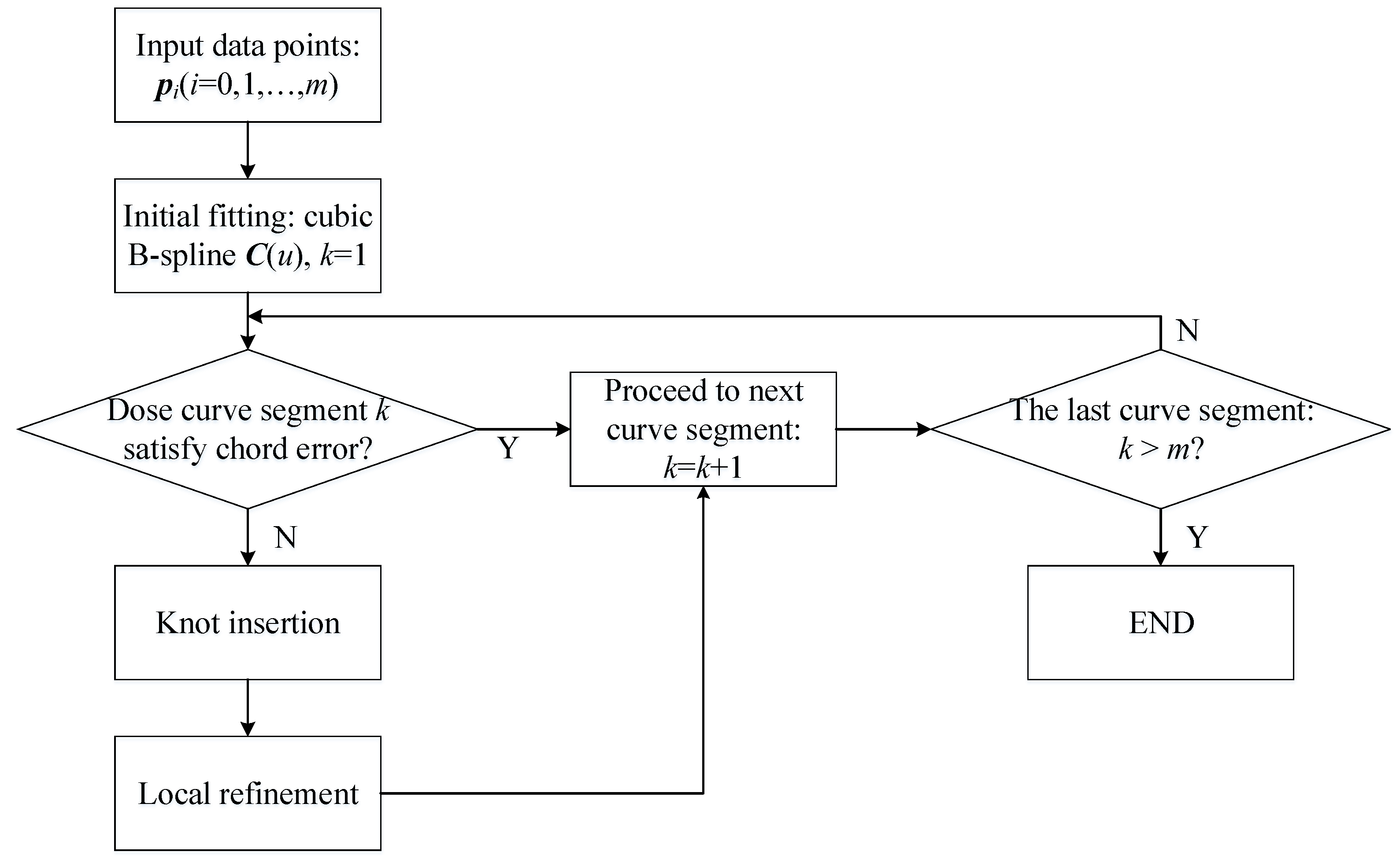
Assuming that the distance between the initial curve in the parameter interval and the corresponding line segment is greater than , the local refinement process is expected to be limited in the parameter interval so that the remaining portion of the curve is not affected.
In order to increase the flexibility of the local curve segment that needs to be refined, control points are added using knots insertion. Let
be the knot inserted to
, the new control points can be calculated as:
where
.
Denote
and
as
and
after knot insertion. Denote the distance between the control point
and
as
.
and
which must be not greater than
due to strong convex hull property of B-spline curves [
33], otherwise it is necessary to insert more knots to
. To keep the portion outside
unchanged, we can only adjust the control points
. If
, replace
with
where
is the unit vector that points from
to
and
is the distance moved along
. Assign
to the unit vector of the direction that is perpendicular to
and
to the value of
. After all the local curve segments are refined, the final curve satisfies the fitting tolerance while maintaining C2-continuity. Flow of the proposed curve-fitting scheme is shown in
Figure 2.
We present a planar example with five points and fitting tolerance of 0.05 mm as a numerical illustration of the proposed curve-fitting scheme. The result of the B-spline curve fitted to five data points is shown in
Figure 3. The initial curve that satisfies point error exceeds chord error bound at segment 1 and segment 2, which are zoomed in to get a clearer view. Then the two segments is locally refined to obtain the final error-constrained curve. The fitting error and curvature results are demonstrated in
Figure 4. As can be seen, the fitting error of the traditional global curve-fitting method exceeds the fitting tolerance. The proposed curve-fitting method, as an improvement of the global curve-fitting method, can get the fitting error strictly under the fitting tolerance. Compare to the local corner-smoothing method, the proposed method has smaller curvature extrema under the same geometric continuity. Notice that the local corner-smoothing method has lower fitting error in most areas because only the corner parts are replaced. The proposed curve-fitting method is more adaptive to micro linear segments whose adjacent corners are very close.
2.2. Tool Orientation Curve-Fitting
The tool orientation data
are expressed by the spherical coordinates
in the WCS. Unlike curve-fitting of the tool-tip position, the tool orientation is fitted to the Cartesian coordinates that map from the given spherical coordinates to ensure that the magnitude of the orientation vector remains unity [
22]. The mapping from the spherical coordinates to the Cartesian coordinates is obtained as follows:
where
and
are actually the rotary drive commands
and
in the MCS respectively. And the inverse mapping is in the following form:
The fitting tolerance of the tool orientation is given as in the WCS. Since the tool orientation is smoothed in the MCS, it is necessary to convert to which denotes the fitting tolerance of the tool orientation in the MCS.
As shown in
Figure 5, we assume
is the orientation position after O rotates
in the WCS and
is the transitional orientation position that rotates
away from the
-axis to reach
. The lengths of edge
,
, and
are obtained as:
Since
,
, and
are extremely small,
,
, and
are approximately collinear. Thus we have
and Equation (
10) can be simplified as:
Because , we have , that is which lead to . Since , the fitting error of the tool orientation is satisfied if . Without loss of generality, let .
The B-spline curve in the
Cartesian plane is obtained with the input of the mapped tool orientation data
and fitting tolerance
according to the procedure in
Section 2.1 as:
The tool orientation spline
in the WCS is obtained using inverse mapping from Equation (
9). It is noteworthy that the number of control points of the fitted curve depends on the initial curve and the fitting tolerance. Therefore the number of control points of the tool orientation is not necessarily the same as the tool-tip position.
3. Synchronization-Integrated Feedrate Scheduling
Since the tool-tip position and tool orientation are fitted independently in different coordinates, the synchronization and feedrate scheduling are necessary for curve interpolation. In this section, synchronization-integrated feedrate scheduling method is presented to ensure that the tool-tip position motion and tool orientation motion are synchronized and smooth. Feedrate scheduling of the tool-tip position is conducted firstly to address the axial kinematic constraints. Then the tool orientation feedrate is obtained by feedrate deformation method to guarantee smooth rotary motion as well as to share the same motion time with the tool-tip position segment by segment. Thus, the synchronization and feedrate scheduling is implemented in one procedure.
3.1. Feedrate Scheduling for Tool-Tip Position
The goal of feedrate scheduling is to find a smooth interpolation under machining constraints. Usually, the interpolation chord error, the axial kinematics and the tangential kinematics are important constraints for high speed and high accuracy machining. Under the circumstances, the interpolation error, the axial velocities and accelerations are considered to determine the allowable feedrate along the tool-tip position curve . Then the feedrate is scheduled using the S-shape jerk-limited method taking tangential acceleration and jerk into account.
The interpolation chord error along
at the parameter value
u can be approximated as [
25]:
where
T is the interpolation period,
is the curvature radius, and
is the feedrate at the parameter value
u. Hence the interpolation chord error limited feedrate can be obtained as:
where
is the defined limitation of interpolation error. Further, the feedrate in the curve parameter domain can be expressed as:
Denote
as a representation of transition between time domain
t and curve parameter domain
u, and Equation (
14) can be converted to:
The velocity of each axis can be calculated as:
where
represents the drive displacement. If the maximum velocity of each axis is set as
, the axial velocity constraint is written as:
The acceleration of each axis can be calculated as:
If the maximum velocity of each axis is set as
, the axial velocity constraints can be written as:
The parameter interval of the tool-tip curve
is divided into N equal sub-intervals at
. Using the monotonic rational quadratic spline proposed by Fleisig and Spence [
34], the discrete parameter value
of the tool orientation corresponding to
is computed. When
N is large enough, the length of the parameter sub-interval is so small that
in Equations (17) and (19) can be approximated using the finite differential method. We can address the interpolation chord error, the axial velocities and the axial acceleration constraints as an optimization problem with the objective of
and constraints from Equations (16), (18) and (20). By solving the optimization problem, the allowable discrete feedrate values
is acquired. Then the feedrate of the tool-tip position is generated utilizing the curve splitting and bi-directional scanning techniques.
3.2. Feedrate Deformation for Tool Orientation to Achieve Synchronization
The tool-tip position curve at the curve segment joint parameters and the tool orientation curve at the parameter are synchronized spontaneously. Since the feedrate scheduling of the tool-tip position is completed, the motion time along the tool-tip curve in the parameter interval is fixed. Thus the motion time along the tool orientation curve in the parameter interval must be equal to to achieve synchronization. The tangential acceleration and jerk are set to zero at the joint parameters so that the tool-tip position and tool orientation motion are smooth.
Based on these principles, a feedrate deformation method is presented to generate the feedrate of the tool orientation. We take the tool-tip feedrate profile with seven phases in as an illustration. The durations of the seven phases are computed by the start and end feedrate
and
, the maximum feedrate
, the tangential acceleration
and jerk
and the arc-length
:
where
represents the acceleration time,
represents the deceleration time. Denote the constant feedrate duration
as
. The feed displacement is calculated as:
The goal of feedrate deformation is to generate a tool orientation feedrate profile segment by segment with the same motion time as tool-tip position and nominal orientation displacement while keep tangential kinematics under constraint. Given the tool orientation start feedrate
, the tool orientation segmented arc-length
, the feedrate deformation begins with computing the new constant feedrate derived form Equation (
22):
where
is user-defined and
,
and
are the same as tool-tip position. By adjusting
k, different constant feedrates can be obtained to meet the tangential constraints. The updated tangential acceleration and jerk is calculated as:
If
or
still exceed the tangential constraint, we can consider stretching the acceleration time to
and then compute a new constant feedrate so that
and
are reduced. The deceleration process can be handled in the same way.
Figure 6 is an illustration of the feedrate deformation method. The orientation feedrate profile is obtained from deformation of the position feedrate profile so that they share the same motion time but get through respective displacements to reach a specific synchronized cutter location.
With the new constant feedrate, tangential acceleration and jerk, the tool orientation feed time is adjusted to match the tool-tip position feed time while the segmented arc-length remains the same. As a consequence, the tool-tip position and tool orientation arrive at specific points simultaneously where the two curves are synchronized.
4. Simulation and Experiment Validations
The feasibility and effectiveness of the proposed method is validated by simulations on a computer with 4.0 GHz CPU and 8GB RAM and experiments on a five-axis table-tilting machine tool (model of the machine tool) with two rotary axes of A and C whose configuration is illustrated in
Figure 7.
The inverse kinematic transformation of the experimental machine tool is:
where
mm is the offset distance between A-axis and C-axis in the direction of z-axis. The machine is controlled by a TwinCAT-based CNC system with the sampling period of 1 ms. In order to formulate the feedrate profile to S-shape, we add the maximum allowable feedrate for tool-tip position and tool orientation respectively to the predefined constraints which are listed in
Table 1.
The S-shape test piece is used to analyze the performance of the proposed method. The S-shape test piece is defined by two ruled surfaces and is usually used as a representation of the thin-wall workpiece in the aerospace industry. It requires an allowable range of final error from −0.05 mm to +0.05 mm [
35]. We import the CAD model of the test piece shown in
Figure 8a to UG NX 10 to plan the toolpath of the ruled surfaces using five-axis flank milling. The programmed toolpath shown in
Figure 8b is approximated by a series of discrete G01 data points. The five-axis linear-segment toolpath of one of the four corners which consists of 12 G01 data points shown in
Figure 8c is used to demonstrate the effectiveness for the proposed curve-fitting and feedrate scheduling method. The experimental 12 G01 data points is available in
Appendix A Table A1. The tool-tip position fitting error tolerance
is 0.05 mm and the tool orientation fitting error tolerance
is 0.05°.
The results of curve-fitting for the 12-point linear-segment toolpath are shown in
Figure 9 and the corresponding fitting error calculated numerically in the curve parameter space is shown in
Figure 10. From the data, it is evident that the fitting errors of the tool-tip position and of the tool orientation are both under fitting tolerance.
We assign
to compute the discrete locations of the tool-tip position and tool orientation. Then the optimization problem proposed in
Section 3.1 is established and solved using the
solver in Matlab to get the allowable feedrate for the tool-tip position. The feedrate profile of the tool-tip position is obtained using the curve splitting and bi-directional scanning techniques and is shown in
Figure 11. From the data we can tell that the scheduled feedrate profile is smooth and under feedrate restrictions.
The feedrate profiles of the original linear-segment toolpath and the smooth toolpath are compared to show that the total motion duration is reduced by 44.2% from 7.169 s to 3.999 s in
Figure 12. It can also be seen that the tool orientation feedrate is generated sharing the same segmented motion time with the tool-tip position.
The interpolation is conducted to generate reference positions in the WCS, as shown in
Figure 13. From the data, it is evident that the feed process is advanced at high rate except three obtrusive deceleration locations.
The tangential kinematic profiles of the tool-tip position and tool orientation are illustrated in
Figure 14. It can be spotted that all the tangential kinematic profiles meet with the tangential constraints. In
Figure 14c,d, the results of the adjusting techniques mentioned in
Section 3.2 is displayed in the feedrate deformation process.
The traditional parameter synchronization method obtains the tool orientation feedrate after scheduling the tool-tip feedrate by simply sharing the curve parameter. It may cause wild fluctuation in the tool orientation kinematics, as shown in
Figure 15.
Since the interpolation results of the tool-tip position and tool orientation are obtained, the reference axial positions are decided according to inverse kinematic transformation from Equation (
25). Then the reference axial velocities and accelerations are calculated by differentiating the axial positions. The axial velocities and accelerations does not consider axial constraints are shown in
Figure 16. It can be seen that despite a slight improvement of feed time (3.595 s), the acceleration of X-axis and velocity of C-axis exceed the corresponding constraints. The axial velocities and accelerations using the parameter synchronization [
23] are demonstrated in
Figure 17. The accelerations of all axes are far greater than the allowable values at certain locations. The axial velocities and accelerations using the proposed method is depicted in
Figure 18. The data demonstrate that the axial velocities and accelerations are both under limitation. The maximum absolute axial velocities and accelerations using different methods are listed in
Table 2 as an intuitive comparison and the anomalously great values are highlighted in bold, especially for axial accelerations using the parameter synchronization method. As can be seen, the large variations of axial accelerations of the traditional parameter synchronization method come from the wild fluctuation in the tool orientation acceleration as shown in
Figure 15b.
The S-shape test piece made of Aluminum Alloy 1060 is machined on the experimental five-axis table-tilting machine tool with a cutter of diameter 10 mm. The machining process consists of three steps: rough machining, semi-finishing and finishing. The CNC system reads the trajectories using the proposed curve-fitting and feedrate scheduling method and then the axial commands are generated and sent to the controller. The machining results are shown in
Figure 19.
The machining accuracy of the S-shape workpiece is affected by many factors, such as theoretical error, geometric error of the machine tool, and quality of toolpath [
36]. Also, the measurement of freeform workpiece is very complicated. In this experiment, quality of toolpath (fitting error) is mainly concerned. According to drive commands of the machine tool, the real tool-tip position and tool orientation are reversely computed using forward kinematic transformation and the real fitting error in the WCS is calculated. The real maximum and average fitting errors with the traditional parameter synchronization method and the proposed method are demonstrated in
Table 3. Due to large variance of axial kinematics, the maximum and average fitting errors with the traditional parameter synchronization show greater values, especially for the tool orientation (40.0% greater for the maximum fitting error).
The real axial velocities and accelerations shown in
Figure 20 are obtained by differentiating the real axial positions with the sampling period of 1 ms. The real axial velocities and accelerations are both under control and the large fluctuations are further reduced in the real machining process (the acceleration for X-axis is reduced by 44.3%). Experimental results show that the proposed method can generate trajectories with allowable fitting error and smooth motion.
5. Conclusions
This paper proposes a double B-spline curve-fitting and synchronization-integrated feedrate scheduling method for five-axis linear-segment toolpath. The main technical characteristics are as follows—(1) the tool-tip position and tool orientation are fitted by two cubic B-spline curves respectively so that the discontinuities caused by transition corners of five-axis linear-segment toolpath are handled and the fitting error is strictly respected; (2) the axial kinematic constraints are mapped and satisfied in the feedrate scheduling process of the tool-tip position; (3) the synchronization and smooth rotary motion is obtained using feedrate deformation for tool orientation.
Simulations and experiments are carried out to validate the feasibility and effectiveness of the proposed method. For a toolpath of 12 CL data points from the S-shape test piece, the proposed curve-fitting method constrains the fitting error under fitting tolerance. The proposed machining time is reduced significantly by 44.2% in comparison with the original linear-segment toolpath. To verify the smooth motion of the proposed feedrate scheduling method, we compare the proposed method with the method does not consider axial kinematic constraints and the method using parameter synchronization. The results show that the proposed rotary motion is smooth and the axial motions are under kinematic limits. The experiments are conducted on the S-shape test piece. The real tool-tip position and tool orientation are reversely computed using the real axial positions to confirm that the proposed method can generate a smooth toolpath with allowable fitting error. The real axial kinematics are further smoothed in the real machining process.
Despite the progress made in this study, only fitting error and smoothness are considered for the fitted curve. However, the machining accuracy is affected by other factors such as thermal error, geometric errors of machine tool, dynamic error and so forth, and workpiece measurement to evaluate the surface quality directly is not conducted. Therefore, further research should be done in our future study.


