Numerical Estimation of Bonding Force of EPDM Grommet Parts with Hollow Shaft Geometry

Abstract

A grommet is a representative component that fixes the position of a cable. It is made from hyper-elastic materials (rubber), such as ethylene propylene diene monomer (EPDM). The grommet and cable are conventionally fixed through bonding; however, this method has numerous disadvantages that can be improved through relevant research. To apply a fixing method using the elastic force of EPDM rubber, this paper presents an empirical equation for approximating the bonding force of EPDM grommet parts with a hollow shaft geometry. First, tensile tests and the inverse method were used to approximate the basic mechanical properties. The physical properties were derived through basic tests; furthermore, bonding force tests and the inverse method were used on a grommet with a hollow shaft structure. In addition, the Box–Behnken design of experiments was used to predict the amount of change in the bonding force according to the geometry variables. Finally, this study was validated by comparing the approximation results derived through the design of experiments with the analysis and bonding force test results.

1. Introduction

A grommet is typically made from hyper-elastic materials, such as the ethylene propylene diene monomer (EPDM), and is used to secure the position of cables embedded in a vehicle [1,2,3,4,5,6,7]. Because EPDM materials boast excellent elasticity-recovery properties and a high friction coefficient, they are utilized in research on bonded and dustproof parts [8,9,10].

The existing grommet parts are joined to cables through a bonding process. There have also been other problems, such as the generation of hazardous substances during manufacturing or in the process of separating the cable. Accordingly, recent studies have investigated a grommet structure that is physically bonded with the cable.

Physical bonding is more environmentally friendly than chemical bonding and allows for easier dismantling; however, it has the disadvantage of having a low bonding force. In a related study, the bonding force was enhanced by approximating the physical properties of the parts and modifying their shape through finite element analysis (FEA). However, the process of approximating EPDM or rubber depends only on the strain–stress properties and does not consider the interaction with other parts.

Physical properties related to the elasticity of rubber can generally be derived by standard test methods, such as ASTM D412-16 and KS M 6518 [11,12]. In addition, strain–stress data can be approximated through mathematical models, such as the Mooney–Rivlin model [13], Yeoh model [14], Gent model [15], and Ogden model [16,17,18,19,20]. The mathematically defined physical properties are applied to FEA and compared with the experimental results by using the mean square error technique. If the mean square error does not satisfy the reference value, the design of experiments (DOE) or genetic algorithms can be utilized to modify the parameters of the mathematical model, thereby changing the results of the FEA. The technique of repeating this process to reduce the error in the experimental results is referred to as the inverse method and is used to improve the reliability of FEA results. The inverse method is generally used for curve fitting the strain–stress curve for tensile specimens [21,22,23,24]. By defining the property values used in FEA through the inverse method, the thickness, geometry, and analysis conditions of the finite element model can be varied to enhance product performance [25]. However, the performance of rubber parts cannot be sufficiently expressed by elasticity alone. Because not only grommets but also rubber parts are commonly bound to other parts, their interaction with other parts must be considered. By using the inverse method to approximate the elasticity and interaction relationship that affects the bonding force, an accurate prediction of grommet performance can be obtained through FEA.

This paper proposes an experiment and inverse analysis method to approximate the bonding force of a grommet part with a hollow shaft structure. A tensile experiment was performed on the EPDM material, and the inverse method was applied to the displacement-force data. The physical properties of the finite element model are defined through the Ogden model, and the Ogden coefficient values are used as parameters in the inverse method. The bonding force of the grommet was tested, and the inverse method was applied to the displacement-force data. A contact condition was assumed for the relationship between the grommet and cable forming the bonding force. The correlation was assumed to be a scale factor of the bonding force and used as a parameter in the inverse method. Additionally, the Box–Behnken DOE, for approximating the bonding force according to the geometry variables, was used to derive a regression equation. Based on the predicted values of the derived regression equation and the FEA results, as well as the comparison of the experimental results, the bonding force approximation model was validated.

2. EPDM Tensile Specimen and Inverse Method

2.1. Tensile Test

In FEA, hyper-elastic materials, such as EPDM, require force–strain data that can be derived from tensile tests. A tensile specimen was prepared for the material properties test. Figure 1 shows the geometry of the specimen KS M 6518 for the tensile test, and

Table 1. Specimen details.

Symbol	Description	Value	Symbol	Description	Value
$w_0$	Width of grip	25 mm	$l_0$	Total length	100 mm
$w_1$	Width of center	5 mm	$l_1$	Length for grip	15 mm
$R_0$	Inner radius	25 mm	$l_2$	-	25 mm
$R_1$	Radius for center shape	11 mm	$l_3$	Gauge length	20 mm

shows information about the specimen. Figure 2 is a schematic of the machine for tensile testing.

Figure 3 shows the tensile test data in the form of a strain–stress curve. The hyper-elastic material can be approximated by the Ogden and Money–Livelin models to be within the elongation range of 0 to 1 (0% to 100%). Therefore, this study used only those data from the EPDM tensile test data that are within an elongation of 1.

First, to describe the large elastic deformation of the rubber, the elongation ratio ($\lambda$), expressed as a ratio between the original specimen length ($l_0$) and the specimen length after deformation ($l$), can be considered.

$$\lambda =l/l_0$$

(1)

The subscripts 1, 2, and 3 in Ogden’s incompressible model indicate the x-, y-, and z-axis data, respectively. When calculating the strain energy for each axis, the strain hardening exponent ($\alpha$) and material constant ($\mu$) corresponding to the shear stress in micro strain are considered. The total strain energy ($U$) can be derived through this material constant.

$$U=U\left({\lambda }_1, {\lambda }_2, {\lambda }_3\right)={\displaystyle \sum }_{i=1}^N\frac{{\mu }_i}{a_i}\left({\lambda }_1^{a_i}+{\lambda }_2^{a_i}+{\lambda }_3^{a_i}-3\right)$$

(2)

As a function of strain energy, the following relationship can be established for the stress along each axis:

$${\sigma }_1={\lambda }_1\frac{\partial U}{\partial {\lambda }_1}, {\sigma }_2={\lambda }_2\frac{\partial U}{\partial {\lambda }_2}, {\sigma }_3={\lambda }_3\frac{\partial U}{\partial {\lambda }_3}$$

(3)

Substituting Ogden’s incompressible model for the stress equation, Ogden’s stress–elongation ratio relationship for the material is obtained as follows:

$${\sigma }_1={\displaystyle \sum }_{i=1}^N{\mu }_i{\lambda }_1^{a_i}, {\sigma }_2={\displaystyle \sum }_{i=1}^N{\mu }_i{\lambda }_2^{a_i}, {\sigma }_3={\displaystyle \sum }_{i=1}^N{\mu }_i{\lambda }_3^{a_i}$$

(4)

In uniaxial tension, the relationship is ${\sigma }_1=\sigma$, ${\sigma }_2={\sigma }_3=0$, ${\lambda }_1=\lambda$, and ${\lambda }_2={\lambda }_3={\lambda }_1^{-0.5}={\lambda }^{-0.5}$; this can be summarized as follows:

$$\begin{array}{c}{\sigma }_1=\sigma ={\displaystyle {\displaystyle \sum }_{i=1}^N}{\mu }_i{\lambda }^{a_i}\\ {\sigma }_2={\sigma }_3=0={\displaystyle {\displaystyle \sum }_{i=1}^N}{\mu }_i{\lambda }^{-0.5a_i}\end{array}\}$$

(5)

The true stress ($\sigma$) and the nominal stress ($s$) are developed as follows:

$$\sigma ={\displaystyle \sum }_{i=1}^N{\mu }_i{\lambda }^{a_i}$$

(6)

$$s=\sigma {\lambda }^{-1}={\displaystyle \sum }_{i=1}^N{\mu }_i{\lambda }^{a_i-1}$$

(7)

The strain–stress data based on KS M 6518 can be expressed by the Ogden model ($s$), as in the above equation, within an elongation range of 0 to 1. The experimental data can be expressed as the relationship between the elongation ratio and stress, as shown in Figure 4.

Table 2. Curve fitting results for Ogden’s incompressible model.

Symbol	Value	Symbol	Value
$a_1$	−10.88	${\mu }_1$	−56.93
$a_2$	3.376	${\mu }_2$	0.5681
$a_3$	−10.88	${\mu }_3$	56.47

shows the coefficient values of the Ogden model shown in Figure 4.

2.2. Finite Element Analysis

Figure 5 shows the finite element model of the tensile specimen. The elements were created in a three-dimensional form, and their overall average volume was set to $1.5 m{m}^3$. The maximum volume of the element was $3.0m{m}^3$ and the minimum volume of the element was set to $1.0m{m}^3$. The elements are all hexagonal. To reduce the hourglass phenomena that cause errors in stress calculations, all elements were considered with eight integral points in the calculation process. The tensile specimen model was analyzed using LS-Dyna’s explicit solver under the same conditions as shown in Figure 2. In the FEA results, the x-axis values are the maximum displacement in the longitudinal ($l_0$) direction, and the y-axis values are the average values of the forces generated at the nodes of the grip portion. As shown in Figure 6, the FEA results differed considerably from the actual experimental results. For the EPDM physical properties, Ogden’s incompressible model shown in Figure 4 was used.

In the FEA, the numerical analysis was repeated until a suitable Ogden coefficient, wherein the mesh did not behave unstably, was derived.

The fact that the experimental results are similar to the Ogden model derived through numerical analysis does not guarantee the accuracy of FEA. This is demonstrated in Figure 6. The Ogden coefficients derived in Figure 4 were inadequate to represent the actual physical quantities.

The results of the analysis seem to apply the general property polynomial rather than Equation (7). However, in Figure 4, the range of λ values between 1 and 1.1 show a similar trend. Therefore, it can be estimated that the numerically fit physical properties have occurred in the process of being applied to the finite element analysis.

Although the results of the analysis are somewhat inaccurate, the process of deriving the physical properties as shown in Table 2 is meaningful in finding the initial values of the physical properties. The results of FEA can be approximated to the experimental results by changing the physical property coefficients shown in Table 2. This method is called the inverse method.

2.3. Inverse Method

In the FEA, the inverse method was applied to reduce the numerical error. Figure 7 shows the inverse method for the tensile test data. The Ogden coefficients were used as parameters of D-Optimal design of experiments (DOE). DOE affects the Ogden physical properties applied to the FEA. Through the FEA results, a response surface generated through a third-degree polynomial was created. GA (genetic algorithm) was applied to the generated response surface model, and the range and optimal values of each parameter were adjusted. The inverse method process was repeated until the mean square error converged to the reference value. Figure 8 is a graph of the experimental values and analytical results obtained by applying the Ogden coefficients derived through the inverse method. Compared to Figure 6, which shows the results before using the inverse method, the results upon applying the inverse method were observed to be similar to the experimental values. However, the analysis results using the converged factors were somewhat inaccurate in the linear elastic section with a deformation amount of 0 to 5 mm. This error is considered to be an error that occurred because only the biaxial tensile test data were considered.

3. Grommet Mechanical Properties and Inverse Method

3.1. Bonding Force Test

The main indicator of grommet performance is the force that secures the cable position. Figure 9 is a schematic of a hollow shaft grommet to observe the bonding force. The grommet is bonded with the cable by press fitting.

Table 3. Specimen details.

Symbol	Description	Value	Symbol	Description	Value
$d_0$	Outside diameter of grommet	$\varphi 10 mm$	$b_0$	Length of cable	$200 mm$
$d_1$	Inside diameter of grommet	$\varphi 3.7 mm$	$b_1$	Movable length	$100 mm$
$d_2$	Outside diameter of cable	$\varphi 4.3 mm$	$b_2$	Length of grommet	$24 mm$

show the details of specimen.

Figure 10 shows the configuration of the bonding force test for the hollow shaft grommet. The grommet was bonded with the cable. The axial position of the grommet was fixed with a jig. The cable was moved 100 mm vertically toward the top by a tensile tester. As the cable was moved, data on the displacement and force of the tester were measured.

Figure 11 shows the bonding force test data. As indicated by the data, for a displacement of 100 mm or more, the end of the cable is located inside the grommet and the bonding force gradually weakens. Thus, the data within the forced displacement of the cable of 100 mm were set as effective data. The experiment was conducted four times; the data of the third experiment, which were similar to the maximum load averages, were set as the representative values.

3.2. Finite Element Model of Grommet

The cable and grommet were generated through three-dimensional elements. Figure 12 shows the cross-section in the longitudinal direction.

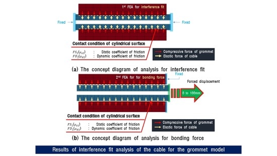
The average volume of the grommet element was set to $2.0 m{m}^3$, and that of the cable element was set to $1.0 m{m}^3$. All elements were applied with fully integrated type to have 16 integral points. The property values and the properties of the tensile specimen were applied in the same way. The inverse method results for the EPDM tensile specimen were applied to the properties of the grommet. For the elastic modulus value (70.0 MPa) and Poisson’s ratio value (0.495) of the cable, the value for normal rubber was used. In the initial state, Grommet’s inner diameter and the cable are not in contact. To simulate the phenomenon in which the grommet is extended by the cable, as shown in Figure 12a, the dynamic relaxation analysis (interference fit analysis) technique provided by LS-Dyna was used. Interference fit analysis is a simulation that derives the penetration distance between the grommet and the cable and pushes it as far as the penetration amount of the grommet. Using the analysis result from Figure 12a, it is set as the initial condition of Figure 12b. The front of the grommet is set to fix, and the cable moves 100 mm in the axial direction. The complex correlation between the grommet and the cable was applied to the static friction coefficient and the dynamic friction coefficient that can be given in the contact conditions of each analysis. The initial values of the friction coefficients were set to 0 and up to 1 in 0.25 intervals. As a result of the analysis in Figure 12b, the cable movement and contact force as shown in Figure 13 were obtained.

3.3. Inverse Method for Bonding Force of Grommet

To observe the bonding force of the grommet, the interference fit analysis and bonding force analysis were conducted continuously. The cable model was forcibly moved 100 mm in the axial direction according to the end time of the analysis. The data extracted from the FEA results were set as the amount of cable movement and force generated at the contact node. Figure 13a shows the analytical results when interaction is not considered, that is, when the scale factor value is not considered. In this case, a contact force of around 1 N was generated. Figure 13b shows the analytical results in which the scale factor of the linear section is set to 0, 0.25, 0.5, 0.75, and 1 in the FEA.

The inverse method for the bonding force was used in the analysis results by applying the scale factor. For the parameters applied to the inverse method, this study considered both the scale factor of the nonlinear section and the scale factor of the linear section in the interference fit analysis, as well as the analysis in which the cable was removed. In addition, the inverse method and tests were performed for cases in which the inner diameter decreased by 8%, remained unchanged, and increased by 8%, by assuming that the scale factor is a function of the grommet inner diameter ($d_1$). When the reduced ratio of the grommet inner diameter is $\eta$, the relationship between $\eta$ and the inner diameter is defined by Equation (8).

$${\mathit{d}}_1+\left({\mathit{d}}_1\times \mathbf{\eta }\%\right)$$

(8)

Figure 14 shows the inverse method, which was very similar to that in Figure 7.

Table 4. Curve fitting results for Ogden’s incompressible model.

Analysis Type	Variable	$\mathbf{Case}\mathbf{1}(\mathit{\eta }=-\mathbf{8})$	$\mathbf{Case}\mathbf{2}(\mathit{\eta }=\mathbf{0})$	$\mathbf{Case}\mathbf{3}(\mathit{\eta }=+\mathbf{8})$
Iteration		7	6	7
Explicit analysis	$F{S}_1$	1.8 × 10−14	0	0.0762635
	$F{D}_1$	0.126171	0.843332	0.274387
Dynamic relaxation analysis	$F{S}_2$	0.422531	0.534858	0.634815
	$F{D}_2$	0.113632	0.6452	0.531285

shows the inverse method results. For the case of lower, unchanged, and higher diameters, the inverse method was repeated seven, six, and seven times, respectively.

Table 4 shows the scale factor values derived through the inverse method. The parameter that impacted the bonding force depending on the change in inner diameter can be considered the scale factor ($F{S}_2$) of the linear section in the interference fit analysis. Before the analysis, this study predicted that the scale factor would increase as the physical tolerance decreased. However, the analysis results indicated the opposite relationship. It can be inferred that other scale factors do not greatly impact the bonding force. The quadratic Equation (9) shows the relationship with the scale factor.

$$F{S}_2=0.001753 {\eta }^2-0.0152 \eta +0.4957$$

(9)

4. Meta-Modeling

4.1. Geometry Variable Configuration and Analysis Using the Box–Behnken Method

The geometry variables of the hollow shaft grommet can be divided into: outer diameter (${\mathit{d}}_0$), inner diameter (${\mathit{d}}_1$), axial length (${\mathit{b}}_2$), and a change in the variables of $\pm 10\%$.

Table 5. Experimental points and results based on the Box–Behnken design.

Order of Execution	Variable Name			Result Value
	${\mathit{b}}_{\mathbf{2}} \left[\mathit{m}\mathit{m}\right]$	${\mathit{d}}_{\mathbf{0}} \left[\mathit{m}\mathit{m}\right]$	${\mathit{d}}_{\mathbf{1}} \left[\mathit{m}\mathit{m}\right]$	$\mathit{W}\mathit{o}\mathit{r}\mathit{k} \left[\mathit{N}·\mathit{m}\mathit{m}\right]$
	${\mathit{x}}_{\mathbf{1}}$	${\mathit{x}}_{\mathbf{2}}$	${\mathit{x}}_{\mathbf{3}}$	R
1	−1	−1	0	3127.5
2	1	-1	0	3831.4
3	−1	1	0	3475.7
4	1	1	0	4392.3
5	−1	0	−1	5677.8
6	1	0	−1	7150.0
7	−1	0	1	1935.1
8	1	0	1	2543.4
9	0	−1	−1	6120.5
10	0	1	−1	6595.0
11	0	−1	1	1052.9
12	0	1	1	2544.5
13	0	0	0	3833.2
14	0	0	0	3833.0
15	0	0	0	3828.3

shows the experimental design based on the Box–Behnken method of response surface analysis and the results according to the set geometry parameters. The Box–Behnken method is a method that aims at optimizing the conditions of the factors that affect the property values and follows the central composite design and the Box–Behnken design [26,27,28]. The geometry variables were coded as −1, 0, 1, and the results were analyzed in the same manner as above.

4.2. Analysis of Analytical Results

Analysis of variance (ANOVA) was conducted for the analytical results according to the variable conditions. Secondary interactions for the inner diameter were confirmed, and terms with low significance were pooled as error terms. ${\mathit{b}}_2$, $d_0$, and $d_1$ were identified as geometry variables with a significant impact; among these, the inner diameter demonstrated the largest influence. The regression Equation (10) was derived from this.

Table 6. ANOVA results.

Source	DF	Adj SS	Adj MS	F-Value	p-Value
Model	4	41,614,451	10,403,613	122.90	0.000
Linear	3	40,884,482	13,628,161	160.99	0.000
$b_2$	1	1,712,255	1,712,255	20.23	0.001
${\mathit{d}}_{\mathbf{0}}$	1	1,033,331	1,033,331	12.21	0.006
${\mathit{d}}_{\mathbf{1}}$	1	38,138,895	38,138,895	450.53	0.000
Square	1	729,969	729,969	8.62	0.015
${\mathit{d}}_{\mathbf{1}}\times {\mathit{d}}_{\mathbf{1}}$	1	729,969	729,969	8.62	0.015
Error	10	846,537	84,654
Lack-of-Fit	8	846,522	105,815	13,808.55	0.000
Pure Error	2	15	8
Total	14	42,460,988

shows the ANOVA results.

Excluding terms with low significance, the regression equation was derived, as in Equation (10). The R-sq and R-sq (adj) of the model were 98.01% and 97.21%, respectively, showing its high explanatory power. Figure 15 shows the work results through the response surface. Figure 15a shows the change in work for the length ($b_2$) and outer diameter ($d_0$) geometry variables; Figure 15b, the length ($b_2$) and outer diameter ($d_1$); and Figure 15c, the change in work according to changes in outer diameter ($d_0$) and inner diameter ($d_1$). The response surface results demonstrate that work is influenced most by $d_1$.

$$R=3760+463b_2+359d_0-2183d_1+442d_1^2$$

(10)

4.3. Verification of Validity

To verify the validity of the derived regression equation, the predicted values and additional samples were prepared, and bonding force tests were conducted.

Table 7. Results of geometry variable modification and bonding force tests to verify the regression equation.

Order of Execution	Variables			Regression EquationResult Value	Finite Element AnalysisResult Value	Bonding Force Test Results
	${\mathit{b}}_{\mathbf{2}}$	${\mathit{d}}_{\mathbf{0}}$	${\mathit{d}}_{\mathbf{1}}$	$\mathit{W}\mathit{o}\mathit{r}\mathit{k}$	$\mathit{W}\mathit{o}\mathit{r}\mathit{k}$	$\mathit{W}\mathit{o}\mathit{r}\mathit{k}$
	$\left[\mathit{m}\mathit{m}\right]$	$\left[\mathit{m}\mathit{m}\right]$	$\left[\mathit{m}\mathit{m}\right]$	$\left[\mathit{N}·\mathit{m}\mathit{m}\right]$	$\left[\mathit{N}·\mathit{m}\mathit{m}\right]$	$\left[\mathit{N}·\mathit{m}\mathit{m}\right]$
	${\mathit{x}}_{\mathbf{1}}$	${\mathit{x}}_{\mathbf{2}}$	${\mathit{x}}_{\mathbf{3}}$	${\mathit{R}}_{\mathbf{2}}$	${\mathit{R}}_{\mathbf{3}}$	${\mathit{R}}_{\mathbf{4}}$
1	0	0	−1	5820.577	4988.759	5414.080
2	0	0	0	3760.000	4153.648	4335.647
3	0	0	1	2280.577	2837.807	2580.570

and Figure 16 show the actual experimental results, FEA values, and values predicted by the regression equation. The experimental values showed an average error of approximately 4.93% in the iterative process. The representative values of the experiment and the FEA results showed an average error of 0.6967%. The representative values of the experiment and the regression equation results showed an average error of 5.8%. The approximation equation showed similar results to the FEA and experimental results.

5. Conclusions

This paper proposed a model for approximating the bonding force of EPDM grommet parts with a hollow shaft geometry. To present the approximation model, EPDM specimens were subject to tensile tests and the inverse method, and the grommet was subject to bonding force tests and the inverse method. The correlation analysis between changes in the geometry variables and bonding force demonstrated that the grommet inner diameter had a greater impact than the grommet length and outer diameter. Furthermore, a correlation equation between the geometry variables and bonding force was derived by using the Box–Behnken DOE.

The findings of this study indicate that the intrinsic properties of EPDM did not greatly affect the bonding force of the grommet. In addition, when the correlation between parts was defined only through the scale factor, the scale factor was observed to increase—to compensate for the physically loosened bonding state. This is contrary to the initial prediction that the scale factor would increase because the interference fit tolerance was given.

Moreover, the fit tolerance between the cable and grommet was found to have a greater impact than the contact area or external design factors. All the analytical data referred to the experimental values, and the approximation equation referred to these analytical data. The bonding force was compared with work; the approximation equation showed an error of approximately 5.8% with the experimental results.

This study was conducted for a grommet with a hollow shaft structure. However, further research is needed for various geometry variables. Furthermore, additional studies on the bonding force considering the anisotropy of the material are needed. If the anisotropic properties are obtained through the uniaxial tensile test, and the inverse analysis is performed with the experimental data, the accuracy of the analysis can be further improved. These research plans can be utilized to provide data to define approximation models of bonding force according to the changes in the grommet geometry variables and the EPDM material. The findings of this study are expected to be of use in the basic design stage for all hyper-elastic materials that have a correlation with other parts.

References

- ASTM. Standard Practice for Rubber and Rubber Latices; ASTM D1418-17; ASTM: West Conshohocken, PA, USA, 2017. [Google Scholar]
- Abou-Helal, M.O.; El-Sabbagh, S.H. A study on the compatibility of NR–EPDM blends using electrical and mechanical techniques. J. Elastomers Plast. 2005, 37, 319–346. [Google Scholar] [CrossRef]
- Kondyurin, A. EPDM rubber modified by nitrogen plasma immersion ion implantation. Materials 2018, 11, 657. [Google Scholar] [CrossRef] [PubMed] [Green Version]
- Ginic-Markovic, M.; Choudhury, N.R.; Dimopoulos, M.; Matisons, J. Adhesion between polyurethane coating and EPDM rubber compound. J. Adhes. Sci. Technol. 2004, 18, 575–596. [Google Scholar] [CrossRef]
- Kwak, S.B.; Choi, N.S.; Choi, Y.J.; Shin, S.M. Nondestructive characterization of degradation of EPDM rubber for automotive radiator hoses. Key Eng. Mater. 2006, 326–328, 565–568. [Google Scholar] [CrossRef]
- Zhao, Q.; Li, X.; Gao, J. Aging of ethylene–propylene–diene monomer (EPDM) in artificial weathering environment. Polym. Degrad. Stab. 2007, 92, 1841–1846. [Google Scholar] [CrossRef]
- Ismail, H.; Pasbakhsh, P.; Ahmad Fauzi, M.N.; Bakar, A.A. Morphological, thermal and tensile properties of halloysite nanotubes filled ethylene propylene diene monomer (EPDM) nanocomposites. Polym. Test. 2008, 27, 841–850. [Google Scholar] [CrossRef]
- Deng, H.; Cheng, L.; Liang, X.; Hayducke, D.; To, A.C. Topology optimization for energy dissipation design of lattice structures through snap-through behavior. Comput. Meth. Appl. Mech. Eng. 2020, 358, 112641. [Google Scholar] [CrossRef]
- Kim, Y.-S.; Hwang, E.-S.; Jeon, E.-S. Optimization of Shape Design of Grommet through Analysis of Physical Properties of EPDM Materials. Appl. Sci. 2019, 9, 133. [Google Scholar] [CrossRef] [Green Version]
- Kim, Y.-S.; Kim, Y.-T.; Jeon, E.-S. Optimization of Accelerator Mixing Ratio for EPDM Rubber Grommet to Improve Mountability Using Mixture Design. Appl. Sci. 2019, 9, 2640. [Google Scholar] [CrossRef] [Green Version]
- ASTM. Standard Test Methods for Vulcanized Rubber and Thermoplastic Elastomers—Tension; ASTM D412-16; ASTM: West Conshohocken, PA, USA, 2016. [Google Scholar]
- Physical Test Methods for Vulcanized Rubber; KS M 6518:2016; Korean Industrial Standards: Seoul, Korea, 2016.
- Mooney, M. A theory of large elastic deformation. J. Appl. Phys. 1940, 11, 582–592. [Google Scholar] [CrossRef]
- Gent, A.N. A new constitutive relation for rubber. Rubber Chem. Technol. 1996, 69, 59–61. [Google Scholar] [CrossRef]
- Yeoh, O.H.; Fleming, P.D. A new attempt to reconcile the statistical and phenomenological theories of rubber elasticity. J. Polym. Sci. B Polym. Phys. 1997, 35, 1919–1932. [Google Scholar] [CrossRef]
- Ogden, R.W. Large deformation isotropic elasticity—On the correlation of theory and experiment for incompressible rubber-like solids. Rubber Chem. Technol. 1973, 46, 398–416. [Google Scholar] [CrossRef]
- Wu, Y.; Wang, H.; Li, A. Parameter Identification Methods for Hyperelastic and Hyper-Viscoelastic Models. Appl. Sci. 2016, 6, 386. [Google Scholar] [CrossRef] [Green Version]
- Lee, G.-B.; Kim, S.-G.; Yoo, Y.-H.; Kang, S.-I.; Oh, J.-G.; Huh, Y.-I.; Jeong, B.-H.; Nah, C.-W. Phase Morphology and Mechanical Properties of Ethylene-Propylene-Diene-Monomer/Fluoroelastomer Blends. Polymer (Korea) 2015, 39, 754–760. [Google Scholar] [CrossRef] [Green Version]
- Gatos, K.G.; Thomann, R.; Karger-Kocsis, J. Characteristics of ethylene propylene diene monomerrubber/organoclay nanocomposites resulting from different processing conditions and formulations. Polym. Int. 2004, 53, 1191–1197. [Google Scholar] [CrossRef]
- Ismail, H.; Shaari, S.M. Curing characteristics, tensile properties and morphology of palm ash/halloysitenanotubes/ethylene-propylene-diene monomer (EPDM) hybrid composites. Polym. Test. 2010, 29, 872–878. [Google Scholar] [CrossRef]
- Zhao, K.; Wang, L.; Chang, Y.; Yan, J. Identification of post-necking stress–strain curve for sheet metals by inverse method. Mech. Mater. 2016, 92, 107–118. [Google Scholar] [CrossRef]
- Zhang, Z.L.; Hauge, M.; Odegard, J.; Thaulow, C. Determining material true stress-strain curve from tensile specimens with rectangular cross-section. Int. J. Solids Struct. 1999, 36, 3497–3516. [Google Scholar] [CrossRef]
- Kim, J.H.; Serpantie, A.; Barlat, F.; Pierron, F.; Lee, M.G. Characterization of the post-necking strain hardening behavior using the virtual fields method. Int. J. Solids Struct. 2013, 50, 3829–3842. [Google Scholar] [CrossRef] [Green Version]
- Joun, M.S.; Eom, J.G.; Lee, M.C. A new method for acquiring true stress–strain curves over a large range of strains using a tensile test and finite element method. Mech. Mater. 2008, 40, 586–593. [Google Scholar] [CrossRef]
- Cho, J.R. Fatigue life prediction and optimum topology design of EPDM weather strip. Finite Elem. Anal. Des. 2012, 60, 57–63. [Google Scholar] [CrossRef]
- Kim, Y.S.; Jeon, E.S.; Kim, D.R. Optimization of process variables for improvement of seat-backboard peel strength using response surface design method. J. Mech. Sci. Technol. 2017, 31, 5915–5920. [Google Scholar] [CrossRef]
- Singh, P.K.; Kumar, S.D.; Patel, D.; Prasad, S. Optimization of vibratory welding process parameters using response surface methodology. J. Mech. Sci. Technol. 2017, 31, 2487–2495. [Google Scholar] [CrossRef]
- Myers, R.H.; Montgomery, D.C.; Anderson-Cook, C.M. Response Surface Methodology: Process and Product Optimization Using Designed Experiments; John Wiley & Sons: Hoboken, NJ, USA, 2016. [Google Scholar]
Figure 1.
Schematic of the KS M 6518 tensile specimen.
Figure 2.
Schematic of the KS M 6518 tensile test.
Figure 3.
Tensile test results.
Figure 4.
Comparison of tensile test results and Ogden’s incompressible model.
Figure 5.
Finite element model for tensile specimen of ethylene propylene diene monomer (EPDM) 60 material.
Figure 6.
Experimental data expressed as points and finite element analysis (FEA) results expressed as curves.
Figure 7.
Fitting procedure of Ogden’s incompressible model using the inverse method.
Figure 8.
Experimental data expressed as points and FEA results expressed as dotted lines.
Figure 9.
Schematic of grommet and cable used for bonding force test.
Figure 10.
Overview of the tensile test required for the bonding force test. (a) Schematic of the grommet bonding force test; (b) Test using the tensile tester.
Figure 11.
Representative values of the bonding force test results and experimental data (data of third experiment).
Figure 12.
Results of interference fit analysis of the cable for the grommet model; (a) The concept diagram of analysis for interference fit; (b) The concept diagram of analysis for bonding force.
Figure 13.
Grommet bonding force test results and FEA process and results; (a) Scale factor value not applied; (b) Scale factor value applied.
Figure 14.
Approximation of grommet bonding force using the inverse method.
Figure 15.
Response surface results of work. (a) Design variable , ; (b) Design variable , ; (c) Design variable , .
Figure 16.
Experimental and FEA results to verify the regression equation. (a) Decrease in inner diameter by 8% (); (b) Normal inner diameter (); (c) Increase in inner diameter by 8% ().