A Dynamic Model for Continuous Lowering Analysis of Deep-Sea Equipment, Based on the Lumped-Mass Method


Abstract
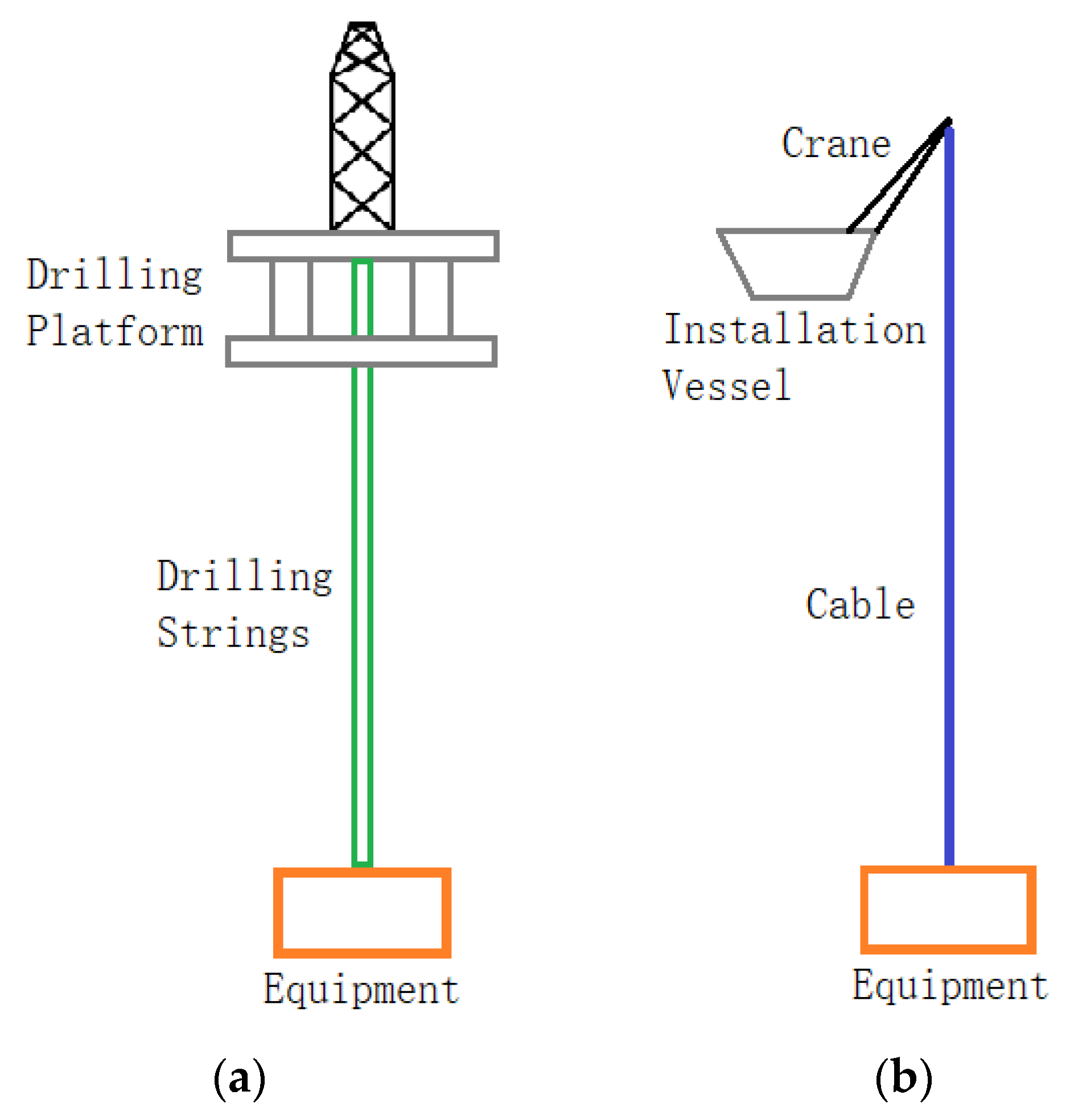
:1. Introduction
2. Mathematical Model and Solution
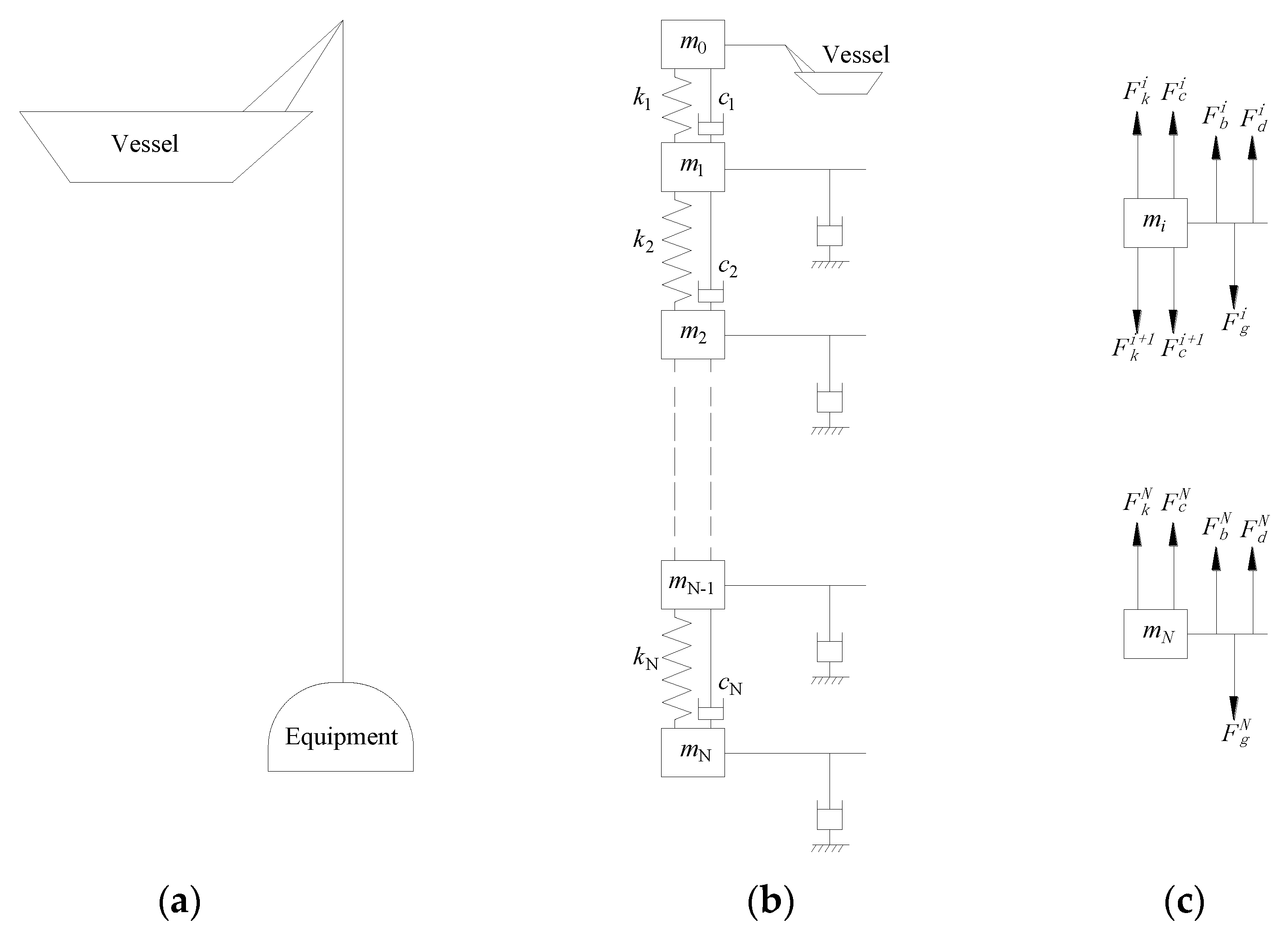
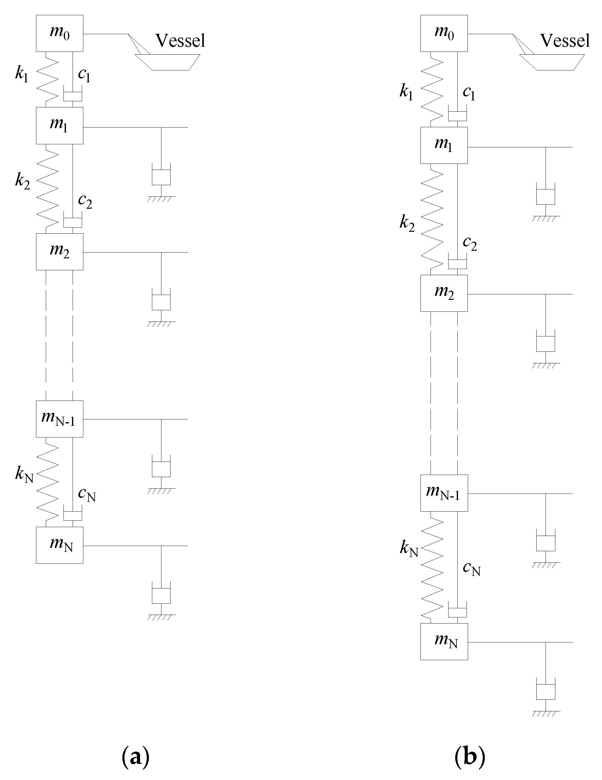
2.1. Mathematical Model
2.2. Numerical Solution
- (1)
- At t0, the beginning of the solution, Equation (15) is solved with the fourth-order Runge–Cutter method to get the displacement and velocity of each mass point, e.g., and .
- (2)
- At , the whole length of the cable is increased by , and then the element length is increased by . Equation (15) is updated according to Appendix A, and solved to get and . Then the traction in the cable can be calculated through Equations (16) and (17).
- (3)
- Step (2) is repeated until the dedicated lowering depth is achieved.
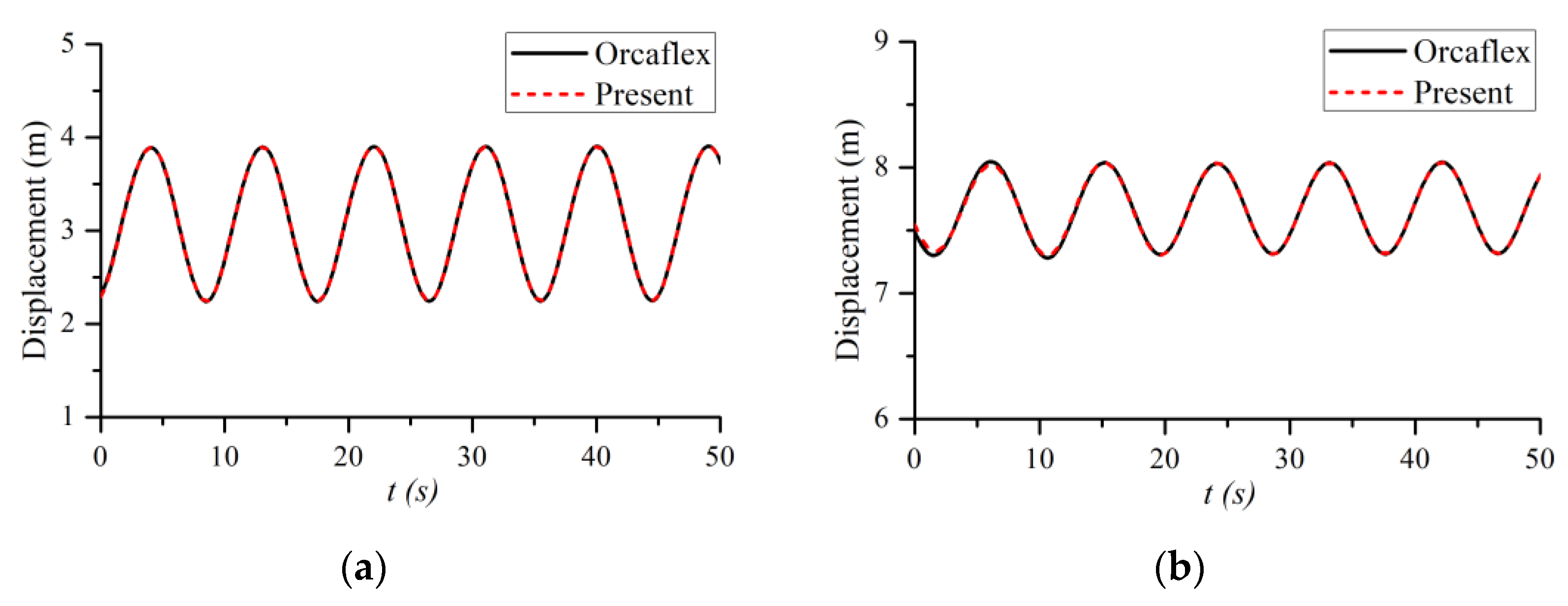
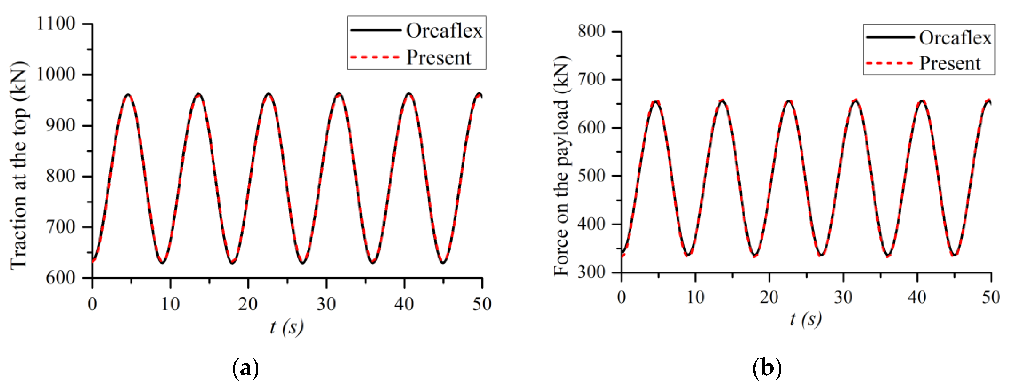
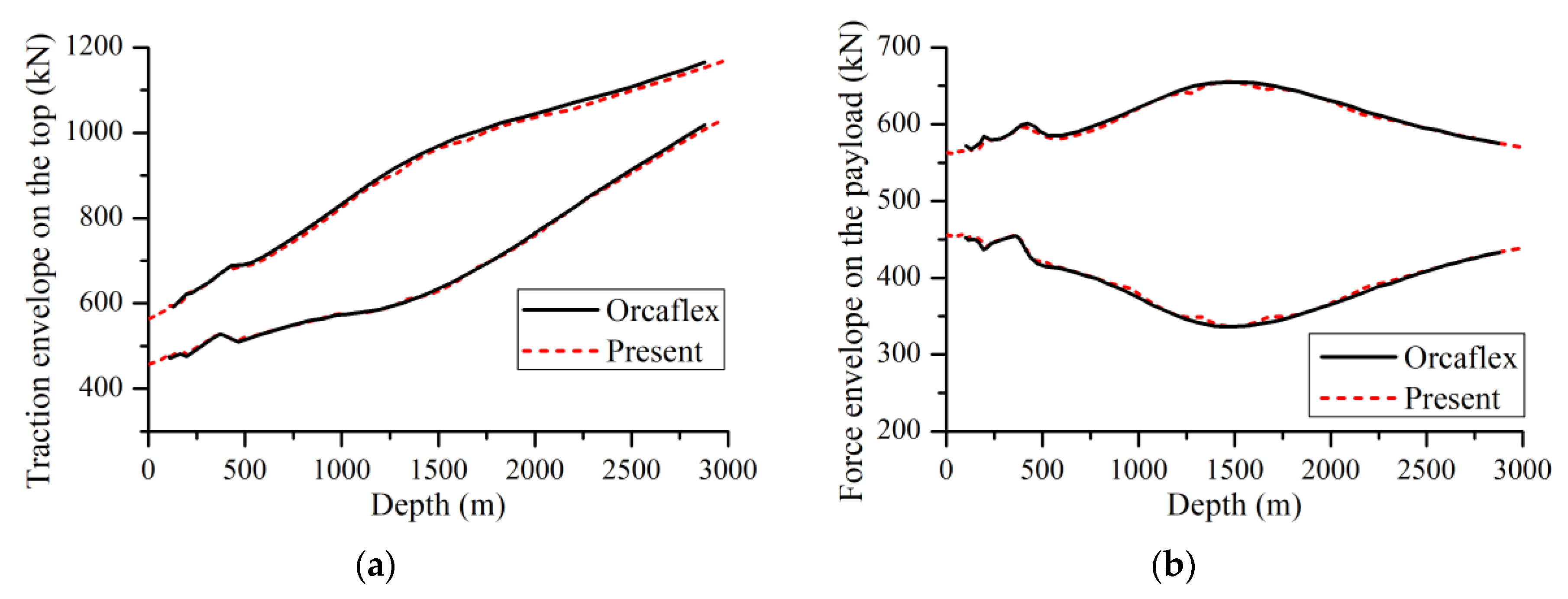
2.3. Model Validation
3. Results and Discussions
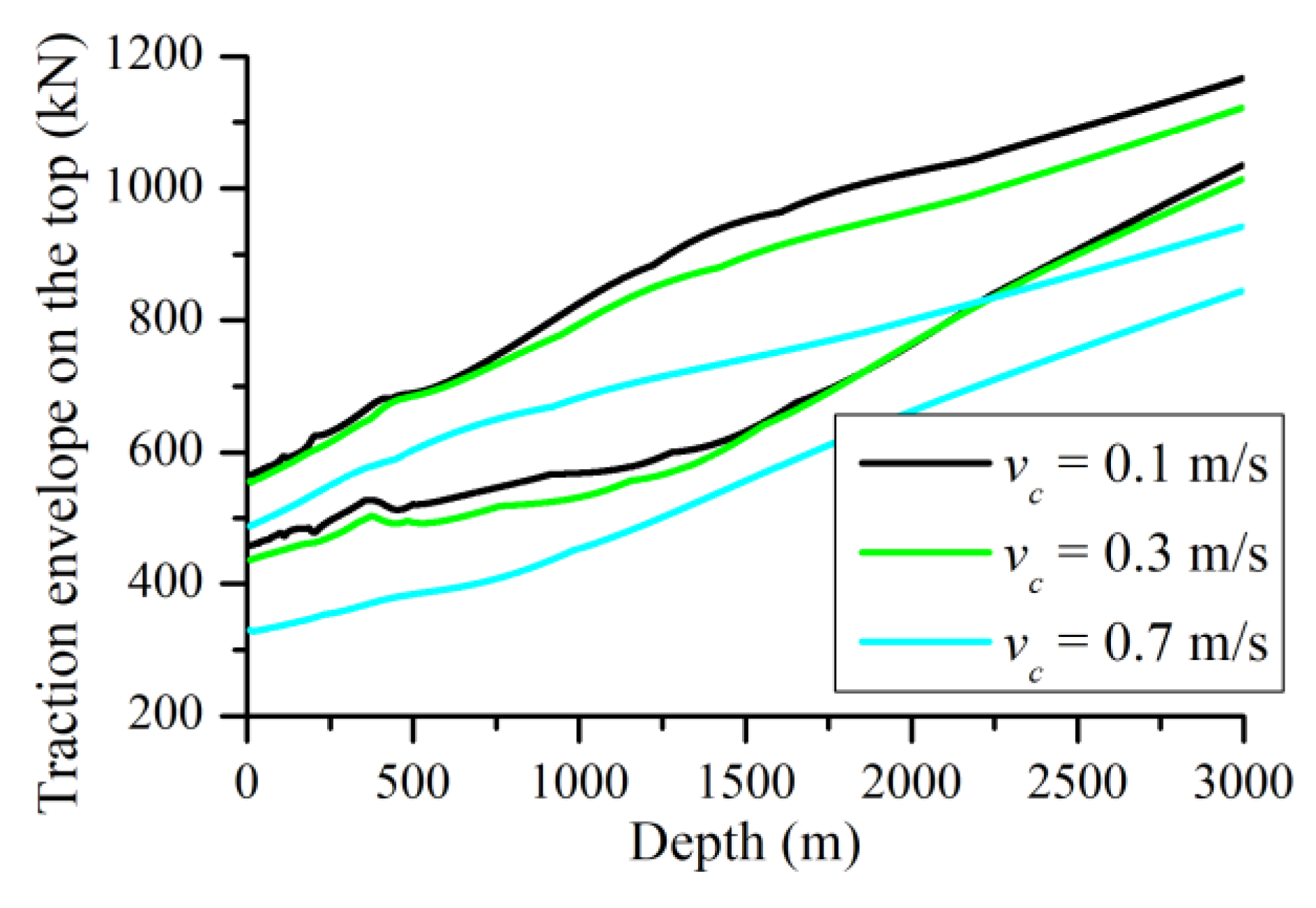
3.1. Lowering Velocity Effect
3.2. Snap Loads
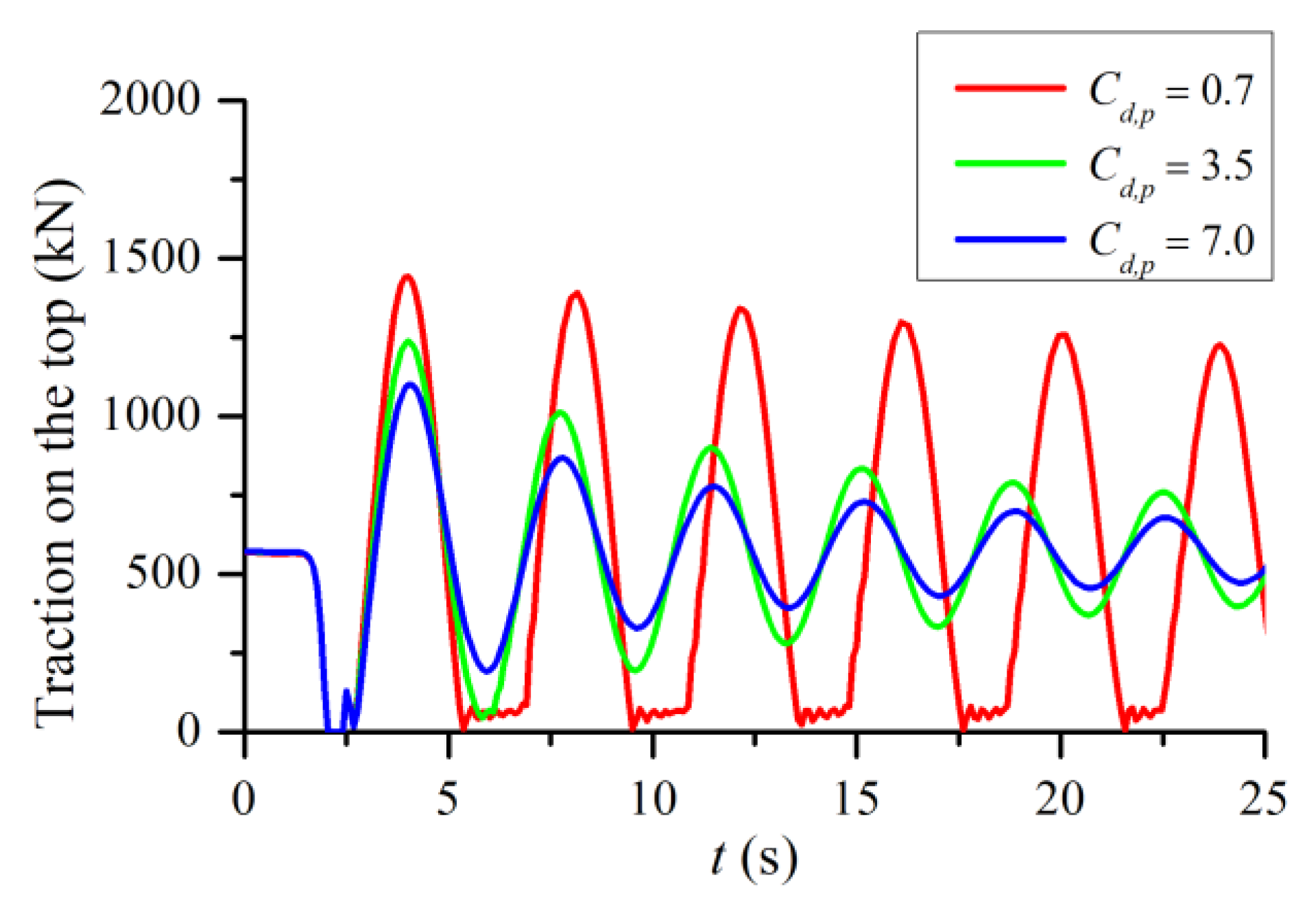
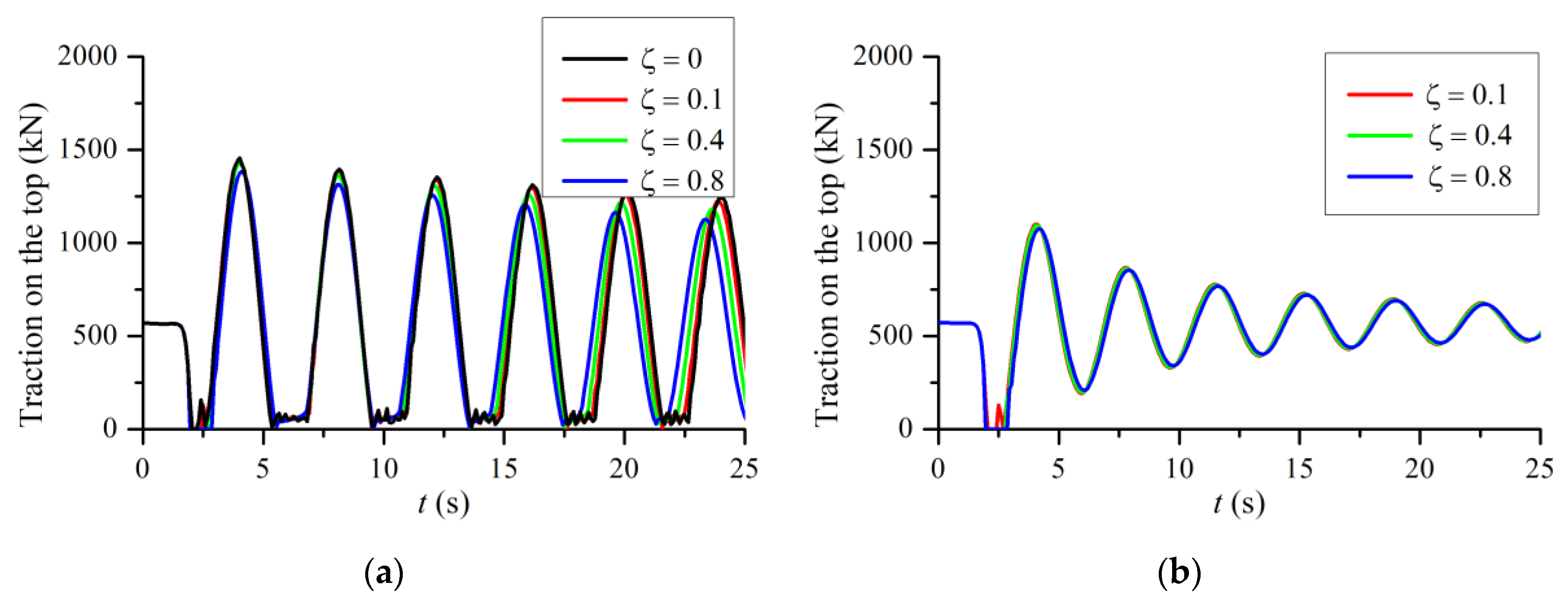
3.3. Damping Effect
3.4. Cable Stiffness Effect
4. Conclusions
Author Contributions
Funding
Acknowledgments
Conflicts of Interest
Appendix A
References
- Wang, Y.; Duan, M.; Liu, H.; Tian, R.; Peng, C. Advances in deepwater structure installation technologies. Underw. Technol. 2017, 34, 83–91. [Google Scholar] [CrossRef]
- Gao, P.; Jin, B.; Zeng, J.; Zhan, Y.; Zhou, H. Numerical analysis of deep-water pipeline abandonment and recovery. J. Mar. Sci. Technol. 2019, 27, 505–512. [Google Scholar]
- Wang, Y.; Tuo, H.; Li, L.; Zhao, Y.; Qin, H.; An, C. Dynamic simulation of installation of the subsea cluster manifold by drilling pipe in deep water based on OrcaFlex. J. Pet. Sci. Eng. 2018, 163, 67–78. [Google Scholar] [CrossRef]
- Zhang, H.; He, Y.; Li, D.; Gu, F.; Li, Q.; Zhang, M. Marine UAV—USV Marsupial Platform: System and Recovery Technic Verification. Appl. Sci. 2020, 10, 1583. [Google Scholar] [CrossRef] [Green Version]
- Roman, D.; Ahilan, R.V. Experience with deepwater installation. Adv. Underw. Technol. 1989, 19, 91–104. [Google Scholar]
- Wu, Y.; Lu, J.; Zhang, C. Study on dynamic characteristics of coupled model for deep-water lifting system. J. Ocean Univ. China 2016, 15, 809–814. [Google Scholar] [CrossRef]
- Zhang, X.; Duan, M.; Mao, D.; Yu, Y.; Yu, J.; Wang, Y. A mathematical model of virtual simulation for deepwater installation of subsea production facilities. Ships Offshore Struct. 2017, 12, 182–195. [Google Scholar] [CrossRef]
- Huang, S.; Vassalos, D. A numerical method for predicting snap loading of marine cables. Appl. Ocean Res. 1993, 15, 235–242. [Google Scholar] [CrossRef]
- Driscoll, F.R.; Lueck, R.G.; Nahon, M. Development and validation of a lumped-mass dynamics model of a deep-sea ROV system. Appl. Ocean Res. 2000, 22, 169–182. [Google Scholar] [CrossRef]
- Zhu, K.Q.; Zheng, D.C.; Cai, Y.; Yu, C.L.; Wang, R.; Liu, Y.L.; Zhang, F. Nonlinear hydrodynamic response of marine cable -body system under random dynamic excitations. J. Hydrodyn. 2009, 21, 851–855. [Google Scholar] [CrossRef]
- Richter, M.; Zeil, F.; Walser, D.; Schneider, K.; Sawodny, O. Modeling offshore ropes for deepwater lifting applications. In Proceedings of the 2016 IEEE International Conference on Advanced Intelligent Mechatronics (AIM), Banff, AB, Canada, 12–15 July 2016; pp. 1222–1227. [Google Scholar]
- Modelling and Analysis of Marine Operations. Available online: https://www.yumpu.com/en/document/view/11798016/dnv-rp-h103-modelling-and-analysis-of-marine-operations (accessed on 11 September 2019).
- Bai, Y.; Ruan, W.; Yuan, S.; He, X.; Fu, J. 3D mechanical analysis of subsea manifold installation by drill pipe in deep water. Ships Offshore Struct. 2014, 9, 333–343. [Google Scholar] [CrossRef]
- Chen, Z.; Zhao, T.; Jiao, J.; Mao, D. Simulation and motion analysis of deepwater manifold lifting. J. Mar. Sci. Technol. 2017, 25, 696–704. [Google Scholar]
- Wang, F.C.; Wang, J.; Tang, K. A finite element based study on lowering operation of subsea massive structure. China Ocean Eng. 2017, 31, 646–652. [Google Scholar] [CrossRef]
- Qin, H.; Liu, J.; Xiao, W.; Wang, B. Quasistatic Nonlinear Analysis of a Drill Pipe in Subsea Xmas Tree Installation. Math. Probl. Eng. 2019, 2019, 4241363. [Google Scholar] [CrossRef]
- Tommasini, R.B.; de Oliveira Carvalho, L.; Pavanello, R. A dynamic model to evaluate the influence of the laying or retrieval speed on the installation and recovery of subsea equipment. Appl. Ocean Res. 2018, 77, 34–44. [Google Scholar] [CrossRef]
- Wang, P.-H.; Fung, R.-F.; Lee, M.-J. Finite element analysis of a three-dimensional underwater cable with time-dependent length. J. Sound Vib. 1998, 209, 223–249. [Google Scholar] [CrossRef]
- Moustafa, K.A.F.; Gad, E.H.; El-Moneer, A.M.A.; Ismail, M.I.S. Modelling and control of overhead cranes with flexible variable-length cable by finite element method. Trans. Inst. Meas. Control 2005, 27, 1–20. [Google Scholar] [CrossRef]
- Hu, Y.; Cao, J.; Yao, B.; Zeng, Z.; Lian, L. Dynamic behaviors of a marine riser with variable length during the installation of a subsea production tree. J. Mar. Sci. Technol. 2018, 23, 378–388. [Google Scholar] [CrossRef]
- Stylianou, M.; Tabarrok, B. Finite Element Analysis of an Axially Moving Beam, Part I: Time Integration. J. Sound Vib. 1994, 178, 433–453. [Google Scholar] [CrossRef]
- Hu, X.Z.; Liu, S.J. Numerical simulation of deepwater deployment for offshore structures with deploying cables. J. Cent. South Univ. 2015, 22, 922–930. [Google Scholar] [CrossRef]
- Thurston, K.W.; Swanson, R.C.; Kopp, F. Statistical characterization of slacking and snap loading during offshore lifting and lowering in a wave environment. In Proceedings of the ASME 2011 30th International Conference on Ocean, Offshore and Arctic Engineering, Rotterdam, The Netherlands, 19–24 June 2011; pp. 269–277. [Google Scholar]
- Orcina Ltd. OrcaFlex Documentation (Version 10.3d). Available online: https://www.orcina.com/resources/documentation/ (accessed on 11 September 2019).
- Driscoll, F.R.; Lueck, R.G.; Nahon, M. The motion of a deep-sea remotely operated vehicle system. Part 1: Motion observations. Ocean Eng. 2000, 27, 29–56. [Google Scholar] [CrossRef]
- Raman-Nair, W.; Baddour, R.E. Three-dimensional dynamics of a flexible marine riser undergoing large elastic deformations. Multibody Syst. Dyn. 2003, 10, 393–423. [Google Scholar] [CrossRef]
- Feyrer, K. Wire Ropes—Tension, Endurance, Reliability; Springer: Berlin/Heidelberg, Germany, 2015; ISBN 978-3-642-54996-0. [Google Scholar]
- Weller, S.D.; Johanning, L.; Davies, P.; Banfield, S.J. Synthetic mooring ropes for marine renewable energy applications. Renew. Energy 2015, 83, 1268–1278. [Google Scholar] [CrossRef] [Green Version]


| Parameter | Value | |
|---|---|---|
| Cable | Linear mass, | 24.6 kg/m |
| Cross-section area, A | 4098 mm2 | |
| Axial stiffness product, EA | 315 MN | |
| Equivalent diameter, Dr | 72.23 mm | |
| Drag coefficient, | 0.7 | |
| Damping ratio, | 0.1 | |
| Equipment | Mass, mp | 60 t |
| Volume, Vp | 7.63 m3 | |
| Vertical projected Area, Ap | 56.95 m2 | |
| Added mass, | 300 t | |
| Drag coefficient, | 7 | |
© 2020 by the authors. Licensee MDPI, Basel, Switzerland. This article is an open access article distributed under the terms and conditions of the Creative Commons Attribution (CC BY) license (http://creativecommons.org/licenses/by/4.0/).
Share and Cite
Gao, P.; Yan, K.; Ni, M.; Fu, X.; Liu, Z. A Dynamic Model for Continuous Lowering Analysis of Deep-Sea Equipment, Based on the Lumped-Mass Method. Appl. Sci. 2020, 10, 3177. https://doi.org/10.3390/app10093177
Gao P, Yan K, Ni M, Fu X, Liu Z. A Dynamic Model for Continuous Lowering Analysis of Deep-Sea Equipment, Based on the Lumped-Mass Method. Applied Sciences. 2020; 10(9):3177. https://doi.org/10.3390/app10093177
Chicago/Turabian StyleGao, Pan, Keliang Yan, Mingchen Ni, Xuehua Fu, and Zhihui Liu. 2020. "A Dynamic Model for Continuous Lowering Analysis of Deep-Sea Equipment, Based on the Lumped-Mass Method" Applied Sciences 10, no. 9: 3177. https://doi.org/10.3390/app10093177