A Comparative Study of Weighting Methods for Local Reference Frame

Abstract

In the field of photogrammetric engineering, computer vision, and graphics, local shape description is an active research area. A wide variety of local shape descriptors (LSDs) have been designed for different applications, such as shape retrieval, object recognition, and 3D registration. The local reference frame (LRF) is an important component of the LSD. Its repeatability and robustness directly influence the descriptiveness and robustness of the LSD. Several weighting methods have been proposed to improve the repeatability and robustness of the LRF. However, no comprehensive comparison has been implemented to evaluate their performance under different data modalities and nuisances. In this paper, we focus on the comparison of weighting methods by using six datasets with different data modalities and application contexts. We evaluate the repeatability of the LRF under different nuisances, including occlusion, clutter, partial overlap, varying support radii, Gaussian noise, shot noise, point density variation, and keypoint localization error. Through the experiments, the traits, advantages, and disadvantages of weighting methods are summarized.

1. Introduction

Local shape description has been proved to be very successful in the field of photogrammetric engineering, computer vision and graphics. Numerous applications are performed by the local shape description, such as 3D object recognition [1,2,3], simultaneous localization and mapping [4], 3D modeling and scene reconstruction [5,6], shape retrieval [7], and 3D object categorization [8]. In comparison with the global shape descriptor, the local shape descriptor (LSD), which is an important component in the local shape description, holds a number of advantages, including being robust against clutter, occlusion, and missing regions [9]. This leads to that many scholars start to do research on the LSD.

A large number of LSDs have been proposed, which encode the geometric information of the local neighborhood around a specific keypoint by calculating geometric features such as distance [10], local depth [11], and normal deviation [12]. Essentially, the LSD should be invariant to rigid transformation, because point-to-point correspondences are established by matching the LSDs. However, in real applications, the LSD is easily influenced by noise, point density variation, clutter, occlusion, and missing regions. Therefore, an ideal LSD should have the ability to resist these nuisances. Many efforts have been made to deal with these difficulties, such as signature of histograms of orientations (SHOT) [13], rotational projection statistics (RoPS) [1], Tri-Spin-Image (TriSI) [14], and rotational contour signatures (RCS) [15]. These descriptors can be broadly classified into two categories: with or without a local reference frame (LRF). The descriptors without LRF (e.g., spin image [16] and fast point features histograms (FPFH) [17] mainly take the geometric information into consideration but discard the spatial information, thus they usually suffer from low descriptiveness. In contrast, the LRF-based descriptors (e.g., RoPS and TriSI) first build an LRF for the local surface and then characterize the geometric and spatial information with respect to the LRF [18]. A comprehensively comparative study of several LSDs had been performed, and the results showed that the LRF-based descriptors generally outperform those descriptors without LRF in most public datasets [19].

An LRF built on the local surface is a 3D coordinate system independent of the world coordinate system. The aim of building the LRF for the LSD is at least twofold. The first is to make the LSD invariant to rigid transformation, because the LRF is independent of the world coordinate system. The second is to provide fully spatial information for local shape description. This makes the descriptors with LRF more descriptive. As an important component of the LSD, the repeatability and robustness of the LRF directly affect the descriptiveness and robustness of the LSD. Large LRF errors could result in very poor descriptor matching performance [20].

In addition, the LRF also has many other uses. For example, in reference [21], the 1-point random sample consensus (RANSAC) algorithm was proposed to produce robust transformation parameters. A pair of points rather than three pairs of points are used to calculate the transformation parameters because the LRFs of the pair of points can also provide convenience for the calculation of the transformation parameters. This largely reduces the computational complexity. In reference [22], the 3D Hough voting method based on the LRF was proposed to detect 3D objects by using a set of transformations, and in reference [23], the authors used the LRF to remove outliers for shape correspondence problems. The performance of all these methods largely depends on a repeatable and robust LRF.

In order to improve the descriptor matching performance, a wide variety of LRF methods have been proposed. For instance, an LRF method was proposed in reference [13], in which a weighting method was developed to increase repeatability of the LRF in the presence of clutter, and the sign ambiguity of all the axes of the LRF was eliminated for the first time. In reference [24], the authors proposed an LRF method for point cloud data and developed a different weighting method to improve the robustness of the LRF to occlusion and clutter. In reference [1], an LRF method was formulated for dealing with triangular mesh data. In reference [25], an evaluation study of six LRF methods was presented in registration and object recognition context, and a novel LRF method was proposed. Only a small subset of the neighboring points around keypoint were used to determine the z-axis, and only a subset of the points lying at the periphery of the local surface were used to determine the x-axis. Subsequently, in reference [18], an LRF method was also proposed, in which the neighboring points with distances to the keypoint being smaller than a threshold were used to determine the z-axis, and all the points in the local neighborhood were projected on the tangent plane of keypoint to obtain the projection vectors, which were then integrated to form the x-axis. The y-axis was determined as the cross-product of the other two axes. In reference [20], these methods were classified into two categories: covariance analysis (CA)-based and geometric attribute (GA)-based methods, and a comprehensive performance assessment of eight LRF methods was also presented. The CA-based methods use all the neighboring points to construct the covariance matrix. The x, y, and z axes of the LRF are obtained by performing the eigenvalue decomposition on the covariance matrix. In contrast, the GA-based methods exploit a subset of the neighboring points to get the z-axis. Then, the x-axis is achieved according to geometric attributes (e.g., signed distance [25]). Finally, the y-axis is obtained by the cross-product of the x and z axes. The experimental results showed that no method is always suitable for different data modalities and application scenarios, and the GA-based methods are generally more time consuming compared to the CA-based methods.

Although the comparative studies of both the LSDs and the LRF methods have been presented in the literature, the comparative study of weighting methods for the LRF has not been conducted. The performance of the LRF is affected by multiple factors, so comparing the LRF methods directly is very hard to determine which factors make an improvement to the LRF. A weighting method plays an important role in an LRF method. Assigning proper weight values to the points in the neighborhood can improve the repeatability and robustness of the LRF. Therefore, in this paper, we focus on the comparison of weighting methods. Majority of these methods calculate the weight values for the points in the local neighborhood according to the distances from the keypoint to these points, but which methods are better is unknown. In this paper, five weighting methods are compared, and a quantitative assessment of them is presented. Six datasets with different data modalities and application contexts are selected to perform the comparative study. The repeatability of the LRF against various nuisances is tested. In addition, the Gaussian function is introduced to build the LRF. Unlike other weighting methods, as long as the weighting function is determined, the weight of each point is fixed. In the Gaussian function, the weight of each point can be changed to adjust its contribution to the LRF. Through the comparative study, the main conclusions are summarized as follows:

(1)

When the wights of the distant points in the local neighborhood are too large, the LRF is sensitive to occlusion, clutter, partial overlap, noise, outliers, and keypoint localization error. By contrast, when the wights of the distant points are too small, the LRF is susceptible to noise, varying point density, and keypoint localization error.

(2)

The weighting method should be mainly designed to achieve the robustness to noise and keypoint localization error. Then, it should be properly adjusted to get a balanced robustness to noise, keypoint localization error, and shape incompleteness. The robustness to point density variation and outliers should be obtained by extra methods.

(3)

No method is generalized, but the GF can always get good performance on different data modalities by changing the value of the Gaussian parameter. Therefore, GF can be regarded as a generalized method.

The remainder of this paper is organized as follows. In Section 2, five weighting methods are reviewed. The evaluation methodology is described with details in Section 3. The experimental results and analysis are presented in Section 4. In Section 5, the conclusion is drawn.

2. Overview of Five Weighting Methods

The weighting methods are mainly related to the CA-based methods, so we employ the CA-based methods to perform the comparative study. Furthermore, the CA-based methods generally have higher computational efficiency in comparison with the GA-based methods and are easy to implement. The sign disambiguation technique [13] is applied to eliminate the sign ambiguity of the LRF for all the considered methods because our aim is to compare the weighting methods. In addition, we also use the keypoint to replace the barycenter when computing the covariance matrix, as proposed in reference [13]. The process diagram of building an LRF is shown in Figure 1.

The covariance matrix is computed as

$$\mathit{C}(\mathit{p})=\frac{1}{{\displaystyle \sum _{{\mathit{q}}_i\in N(\mathit{p})}{w}_{q_i}}}{\displaystyle \sum _{{\mathit{q}}_i\in N(\mathit{p})}{w}_{q_i}({\mathit{q}}_i-\mathit{p}){({\mathit{q}}_i-\mathit{p})}^T},$$

(1)

where $\mathit{p}$ is the keypoint, $N(\mathit{p})$ is the radius neighborhood of $\mathit{p}$, ${\mathit{q}}_i$ is a neighboring point in $N(\mathit{p})$, $w_{q_i}$ is the weight of ${\mathit{q}}_i$. After performing the eigenvalue decomposition on $\mathit{C}(\mathit{p})$, we can obtain three eigenvalues $({\lambda }_1,{\lambda }_2,{\lambda }_3)$ that satisfy ${\lambda }_1\ge {\lambda }_2\ge {\lambda }_3$ and three corresponding eigenvectors $({\mathit{v}}_1,{\mathit{v}}_2,{\mathit{v}}_3)$. The three eigenvectors provide a basis for LRF definition. Specifically, the sign disambiguation technique is applied to redetermine the signs of ${\mathit{v}}_1$ and ${\mathit{v}}_3$, producing two unambiguous vectors ${\tilde{\mathit{v}}}_1$ and ${\tilde{\mathit{v}}}_3$. ${\tilde{\mathit{v}}}_2$ is defined as ${\tilde{\mathit{v}}}_1\times {\tilde{\mathit{v}}}_3$, and ${\tilde{\mathit{v}}}_1$, ${\tilde{\mathit{v}}}_2$ and ${\tilde{\mathit{v}}}_3$ define the directions of the x, y, and z-axes, respectively. Assigning different weights to the points in $N(\mathit{p})$ leads that each point makes different contribution to the covariance matrix. Several methods have been proposed to determine the weights, which are briefly described as follows.

EM [26]: This method does not take any nuisances (e.g., occlusion and clutter) into consideration. The weights for all points are just set as 1. That is

$$w_{q_i}=1.$$

(2)

It means that all points in the local neighborhood make the same contribution to the covariance matrix. In spite of this, the method may obtain more repeatable and robust LRF for some data modalities, as will be shown in Section 4.1.

SHOT [13]: This method treats the local points unequally to enhance the robustness under 3D object recognition scenarios. The weights are computed as

$$w_{q_i}=R-\Vert {\mathit{q}}_i-\mathit{p}\Vert ,$$

(3)

where $R$ is the support radius, $\Vert {\mathit{q}}_i-\mathit{p}\Vert$ is the 3D Euclidean distance between ${\mathit{q}}_i$ and $\mathit{p}$. Thus, the distant points (i.e., the neighboring points have larger distances to the keypoint) are assigned smaller weights. In other words, the contributions of the distant points to the covariance matrix are weakened. The purpose is to increase repeatability in the presence of clutter.

BSC [24]: Dong et al. developed a different weighting strategy to determine the weights. It also assigns smaller weights to the distant points. The weights are computed as

$$w_{q_i}=\frac{R-\Vert {\mathit{q}}_i-\mathit{p}\Vert }{R}.$$

(4)

This weighting strategy is expected to improve the robustness of the LRF against occlusion and clutter because the distant points are easily influenced by occlusion and clutter. Unlike the SHOT method, this method limits the weight values to be between 0 and 1.

TOLDI [18]: Although the method is designed for a GA-based LRF method, it also computes the weight values according to the distances. Therefore, we also include it in the comparison. By using this method, a CA-based LRF method may obtain the more repeatable and robust LRF, and the information obtained by the comparison also has some reference value for the GA-based methods. The weights are calculated as

$$w_{q_i}={(R-\Vert {\mathit{q}}_i-\mathit{p}\Vert )}^2.$$

(5)

This weighting strategy is designed to improve the robustness of the LRF against clutter, occlusion, and missing regions because the distant points contribute less to the covariance matrix.

Gaussian function (GF) [27]: Levin used the GF in the moving least-squares approach to approximate the local surface. Here, it is introduced to determine the weights for the LRF, because better performance may be obtained by this method. The weights are calculated by

$$w_{q_i}=e^{-{(\frac{\Vert {\mathit{q}}_i-\mathit{p}\Vert }{h})}^2},$$

(6)

where $h=\sigma \cdot R$, and $\sigma$ is the Gaussian parameter. It can be seen from Equation (6) that the weights decrease as the distance increases, so the distant points are assigned smaller weights, similar to SHOT, BSC, and TOLDI. Therefore, this weighting strategy is also useful to improve the robustness of the LRF against clutter, occlusion, and missing regions. However, the introduction of $\sigma$ provides flexibility in the weight assignment. The big value of $\sigma$ slightly weakens the contributions of the distant points, while the small value of $\sigma$ greatly weakens the contributions of the distant points. That is, a better weight assignment would be achieved if the value $\sigma$ is properly selected. In Section 4, five different values of $\sigma$ (i.e., 0.2, 0.4, 0.6, 0.8, and 1) are selected to perform the comparison.

3. Evaluation Methodology

To assess and compare the weighting methods mentioned in Section 2, we chose 6 benchmark datasets, which are described in detail in Section 3.1, to conduct our experiments. Then, the evaluation criterion is described in Section 3.2, which is used to evaluate the repeatability of the LRF.

3.1. Datasets

The selected 6 datasets are Retrieval [28], Laser Scanner [29], Kinect [13], Space Time [28], LiDAR Registration [30], and Kinect Registration [13]. These datasets are acquired by different devices, resulting in different data modalities. The Retrieval dataset is obtained by a Cyberware 3030 MS scanner. It contain 6 noise-free models. The Laser Scanner dataset include 5 models and 50 real scenes, forming 188 model-scene pairs. The real scenes are obtained by a Minolta Vivid 910 scanner. The Kinect dataset is acquired by a Microsoft Kinect sensor. It include 6 models and 16 real scenes, providing 43 model-scene pairs. The Space Time dataset is composed of 8 models and 15 real scenes. This dataset is created by the Space Time Stereo technique. It provide 24 model-scene pairs. The LiDAR Registration dataset is obtained by scanning 4 objects from different views using a Minolta Vivid 910 scanner, deriving 22, 16, 16, and 21 point clouds, respectively. The Kinect Registration dataset consists of 15, 16, 20, 13, 16, and 15 point clouds of 6 objects, which are also acquired by a Microsoft Kinect sensor. The Laser Scanner and LiDAR Registration datasets are high-quality, while the Kinect and Kinect Registration datasets are noisy and sparse. The Space Time dataset is contaminated by noise and outliers. The aim is to make our experiments cover various data modalities (i.e., LiDAR, Kinect and Space Time) and application scenarios (i.e., shape retrieval, 3D object recognition and 3D registration), and different kinds of nuisances, including noise, point density variation, clutter, occlusion, shot noise, and partial overlap (i.e., missing regions) are contained in these datasets. The detailed description of the 6 datasets is listed in

Table 1. Experimental datasets and relevant properties [2 0].

Dataset	Scenario	Challenge	Modality
Retrieval	Retrieval	Gaussian noise and point density variation	LiDAR
Laser Scanner	Object recognition	Clutter and occlusion	LiDAR
Kinect	Object recognition	Clutter, occlusion and real noise	Kinect
Space Time	Object recognition	Clutter, occlusion, real noise, and outliers	Space Time
LiDAR Registration	Registration	Self-occlusion and missing regions	LiDAR
Kinect Registration	Registration	Self-occlusion, missing regions, and real noise	Kinect

, and the examples of some of them are shown in Figure 2. Note that we call 2 input shapes as model and scene for simplicity, though such appellation was originally used for object recognition.

3.2. Evaluation Criterion

In theory, if two LRFs ($\mathit{L}({\mathit{p}}^m)$, $\mathit{L}({\mathit{p}}^s)$) of corresponding keypoints (${\mathit{p}}^m$, ${\mathit{p}}^s$) in the model and scene are error-free, the two LRFs should conform to the equation $\mathit{L}({\mathit{p}}^s)={\mathit{R}}_{GT}\mathit{L}({\mathit{p}}^m)$, where ${\mathit{R}}_{GT}$ is the ground-truth rotation matrix. Therefore, we can use the criteria suggested in reference [1] to measure the error between two LRFs:

$$erro{r}_{{\mathit{p}}^m,{\mathit{p}}^s}=a\cos \left(\frac{trace(\mathit{L}({\mathit{p}}^s)\tilde{\mathit{L}}{({\mathit{p}}^m)}^{-1})-1}{2}\right)\frac{180}{\pi },$$

(7)

where $\tilde{\mathit{L}}({\mathit{p}}^m)={\mathit{R}}_{GT}\mathit{L}({\mathit{p}}^m)$. For each dataset, the ground-truth transformation is known in advance. The transformation of the Retrieval dataset is artificially set and then used to simulate the point clouds of the corresponding scenes. The transformations of the Laser Scanner, Kinect, and Space Time datasets are provided by the publishers. The transformations of the LiDAR Registration and Kinect Registration datasets are obtained by manual alignment.

After computing the errors of all the LRF pairs, we calculate the ratio of the LRF pairs in a dataset whose errors being smaller than 10 degrees by

$$r\mathrm{e}peatability=\frac{N_{10}}{N_t},$$

(8)

where $N_{10}$ denotes the number of the LRF pairs whose errors smaller than 10 degrees, $N_t$ denotes the total number of the LRF pairs.

Eight kinds of nuisances (i.e., Gaussian noise, shot noise (i.e., outliers), point density variation, keypoint localization error, clutter, occlusion, partial overlap, and varying support radii) are tested in this paper. The detailed definition of each nuisance can be found in reference [20].

3.3. Implementation Details

For each dataset, we apply the uniform sampling method [31] to extract 1000 points from the model as the keypoints. Then, the ground-truth transformation is used to transform these keypoints, and these transformed keypoints are used to find the nearest points in the scene. Finally, these nearest points are treated as the corresponding keypoints in the scene. The aim is to remove the effect of keypoint localization error on the LRF because keypoint localization error should be tested independently, as inspired by reference [19]. For the datasets with incomplete shape (i.e., Laser Scanner, Kinect, Space Time, LiDAR Registration, and Kinect Registration), we find out the keypoints in the overlapping region. The LRFs are only calculated on the keypoints in the overlapping region. The support radius $R$ is set as 15pr (pr denotes the point cloud resolution, i.e., the average shortest distance among neighboring points) in all the experiments except the experiments for testing varying support radii.

4. Experimental Results and Analysis

4.1. Test on the Six Datasets

The experimental results of the six datasets are listed in

Table 2. Repeatability of the local reference frame (LRF) tested on the six datasets with different weighting methods. The best results are denoted in bold font for each dataset.

	Retrieval	Laser Scanner	Kinect	Space Time	LiDAR Registration	Kinect Registration
EM	0.4992	0.0998	0.2040	0.2507	0.1079	0.0949
SHOT	0.5121	0.1360	0.1903	0.2517	0.1330	0.0905
BSC	0.5121	0.1360	0.1903	0.2517	0.1330	0.0905
TOLDI	0.4445	0.1386	0.1605	0.2458	0.1391	0.0792
GF($\sigma =0.2$)	0.1930	0.0936	0.0468	0.2189	0.1234	0.0350
GF($\sigma =0.4$)	0.4056	0.1338	0.1414	0.2478	0.1420	0.0751
GF($\sigma =0.6$)	0.5151	0.1292	0.1965	0.2597	0.1289	0.0935
GF($\sigma =0.8$)	0.5238	0.1164	0.2008	0.2565	0.1120	0.0960
GF($\sigma =1$)	0.5175	0.1091	0.2028	0.2508	0.1155	0.0956

. For the Retrieval dataset, the 6 noise-free models are transformed to get 6 scenes by artificially setting the ground-truth transformation. Then the 6 scenes are down-sampled (sampling rate of 7/10), and Gaussian noise (standard deviation of 0.3pr) is added to them. The aim is to create a combination of nuisances. The other datasets are real data obtained by laser scanning devices, so no additional operation is implemented on them. In addition, we recommend that readers first see Section 4.4 to know which weighting method makes the distant points contribute more to the covariance matrix and which weighting method makes them contribute less to the covariance matrix.

From Table 2, we can see that, on the Retrieval dataset, GF($\sigma =0.8$) obtains the best performance, followed by GF($\sigma =1$), GF($\sigma =0.6$), BSC, and SHOT. TOLDI achieve relatively poor performance. For this dataset, the weighting method is used to reduce the effect of Gaussian noise and point density variation. Because there is no clutter, occlusion, and missing region, the contributions of the distant points do not need to be declined. Therefore, the weights of the distant points should be increased. However, as can be seen from the calculated results, EM and GF($\sigma =1$) obtain inferior performance. This indicates that too large contributions of the distant points would also degrade the repeatability of the LRF, even without the effect of clutter, occlusion, and missing region.

On the Laser Scanner and LiDAR Registration datasets, GF($\sigma =0.4$), TOLDI, SHOT, and BSC have relatively good performance, whereas EM obtains poor performance. Both of the two datasets are high-quality, so they are less contaminated by noise. In this case, the contributions of distant points ought to be controlled properly, as will be shown in Section 4.3. Furthermore, their contributions should be weakened to improve the robustness to clutter, occlusion, and missing regions as well. The is the reason why GF($\sigma =0.4$) and TOLDI achieve good performance, while EM and GF($\sigma =1$) obtain poor performance on the two datasets.

For the Kinect and Kinect Registration datasets, the ranking of all the methods changes significantly. The three best methods are GF($\sigma =0.8$), GF($\sigma =1$), and EM, while TOLDI gets a relatively poor performance. In addition to shape incompleteness (i.e., occlusion, clutter, and missing regions), the two datasets are also rather sparse (i.e., the point density variation is obvious) and noisy. Especially for point density variation, the contributions of the distant points should be increased, as will be shown in Section 4.3. TOLDI is sensitive to point density variation, so it exhibits poor repeatability, even under the case with clutter, occlusion, and missing regions.

For the Space Time dataset, the four methods (GF($\sigma =0.6$), GF($\sigma =0.8$), SHOT, and BSC) achieve relatively good performance, among which GF($\sigma =0.6$) is the best one. In this dataset, besides clutter and occlusion, noise and outliers are the main nuisances. For outliers, the weights of the distant points should be reduced, because outliers are far away from the local surface. Moreover, this is helpful in reducing the effect of clutter and occlusion. However, if the weights of the distant points are too small, the LRF is sensitive to noise. Hence, TOLDI and GF($\sigma =0.2$) obtain the worst performance.

Based on the above discussion, we can know that no weighting method is always the best for all the datasets, because different datasets contain different kinds of nuisances, and the levels of nuisances are also different. Additionally, BSC is totally equivalent to SHOT, because the two methods always achieve the same results on the six datasets.

4.2. Repeatability of LRF Under Different Levels of Occlusion, Clutter, and Partial Overlap, as Well as Varying Support Radii

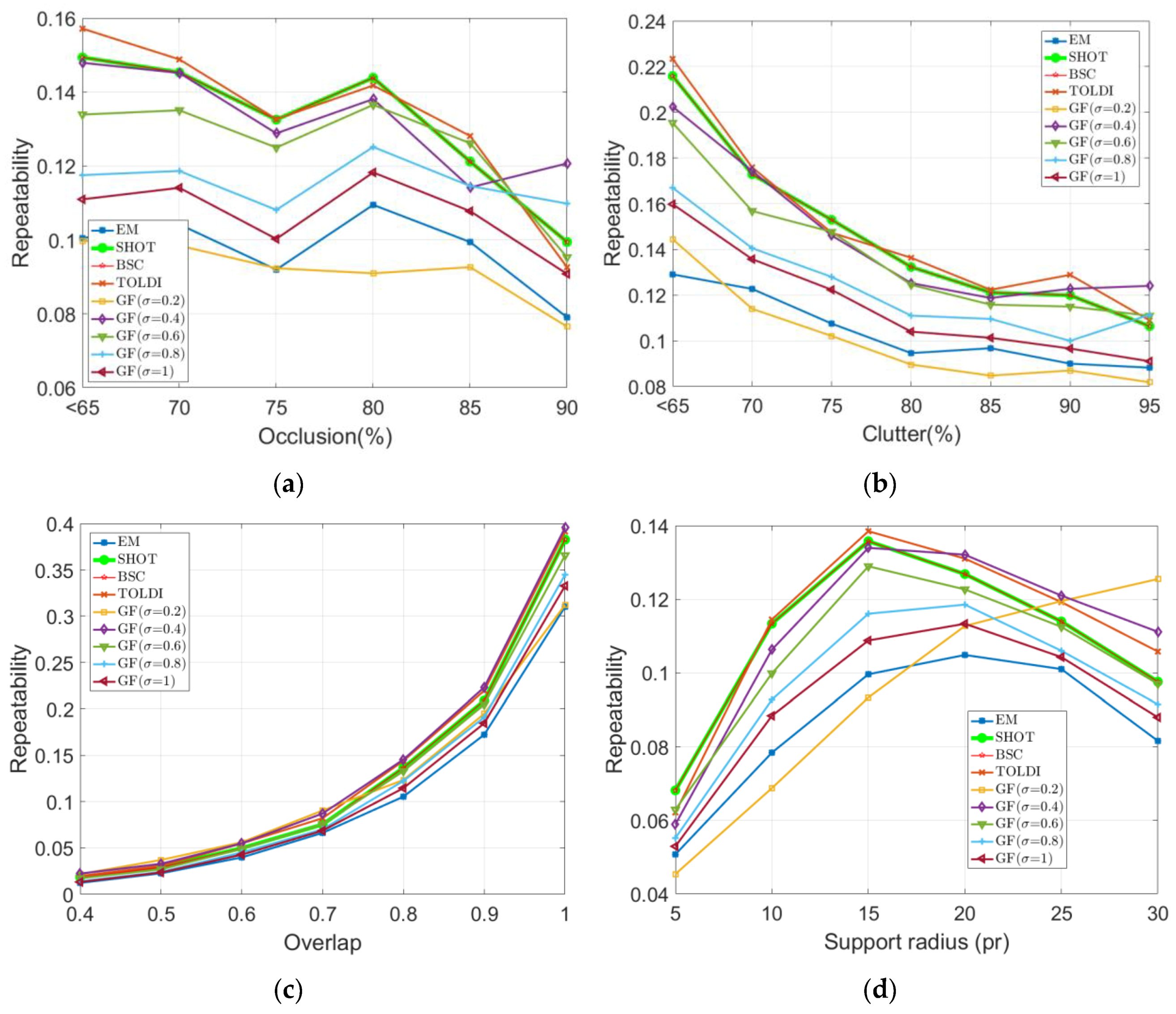
The calculated results under the four nuisances are shown in Figure 3. The three terms (including occlusion, clutter, and varying support radii) are tested on the Laser Scanner dataset. The term (partial overlap) is tested on the LiDAR Registration dataset. For the Laser Scanner dataset, we compute the percentages of occlusion and clutter of each model-scene pair. Then, according to the degree of occlusion, all the model-scene pairs are grouped into 6 clusters, and according to the degree of clutter, they are separated into 7 groups. The partition intervals for occlusion are respectively less than 65%, [65%, 70%), [70%, 75%), [75%, 80%), [80%, 85%) and [85%, 90%), and those for clutter are respectively less than 65%, [65%, 70%), [70%, 75%), [75%, 80%), [80%, 85%), [85%, 90%) and [90%, 95%). For the LiDAR Registration dataset, we compute the degree of overlap of each view pair. Only the view pairs with overlap being more than 0.3 are applied for the experiments. Then, these view pairs are divided into 7 groups according to the degree of overlap, and the partition intervals are (0.3, 0.4], (0.4, 0.5], (0.5, 0.6], (0.6, 0.7], (0.7, 0.8], (0.8, 0.9] and (0.9, 1], respectively. On the test for varying support radii, the radius is set from 5pr to 30pr with a step of 5pr.

As we can see from Figure 3a,b, with the increase of occlusion and clutter, the repeatability of the LRF decreases on the whole. In Figure 3c, the repeatability of the LRF increases as the overlap increases. TOLDI, SHOT, BSC, and GF($\sigma =0.4$) are the best methods under different degrees of occlusion, clutter, or overlap. This indicates that reducing the contributions of the distant points indeed work to enhance the robustness to occlusion, clutter, and missing regions. We can also see that when the degree of occlusion, clutter, or overlap increases, the four methods are always the best. In other words, we do not need to further reduce the weights of the distant points when the degree of occlusion, clutter, or missing regions becomes larger. The weights of the distant points just need to be properly reduced. However, from the results in Table 2, we can know that if the experiments are tested on Kinect and Kinect Registration datasets, which are pretty sparse and noisy, the best methods would be GF($\sigma =0.8$), GF($\sigma =1$) and EM. Therefore, the weighting method should be designed to first reduce the effect of other nuisances (e.g., noise and keypoint localization error). Then, if occlusion, clutter, and missing regions are present, the weighting method should be further adjusted to reduce the effect of these nuisances.

In Figure 3d, TOLDI is the best method when the support radius is 10pr and 15pr, whereas GF($\sigma =0.4$) is the best method when the support radius is 20pr and 25pr. No method is always the best for all the support radii. With the increase of the support radius, the occlusion and clutter near the keypoint are introduced into the local neighborhood. Therefore, the weights of the distant points need to be further reduced. Especially, when the support radius is 30pr, GF($\sigma =0.2$) is the best method, which largely reduces the weights of the distant points. The occlusion and clutter that are far away from keypoint do not affect the repeatability of LRF. This explains why TOLDI, SHOT, BSC, and GF($\sigma =0.4$) always achieve the best performance in Figure 3a,b when the degree of occlusion or clutter increases.

4.3. Repeatability of LRF Under Different Levels of Gaussian Noise, Point Density Variation, Shot Noise, and Keypoint Localization Error

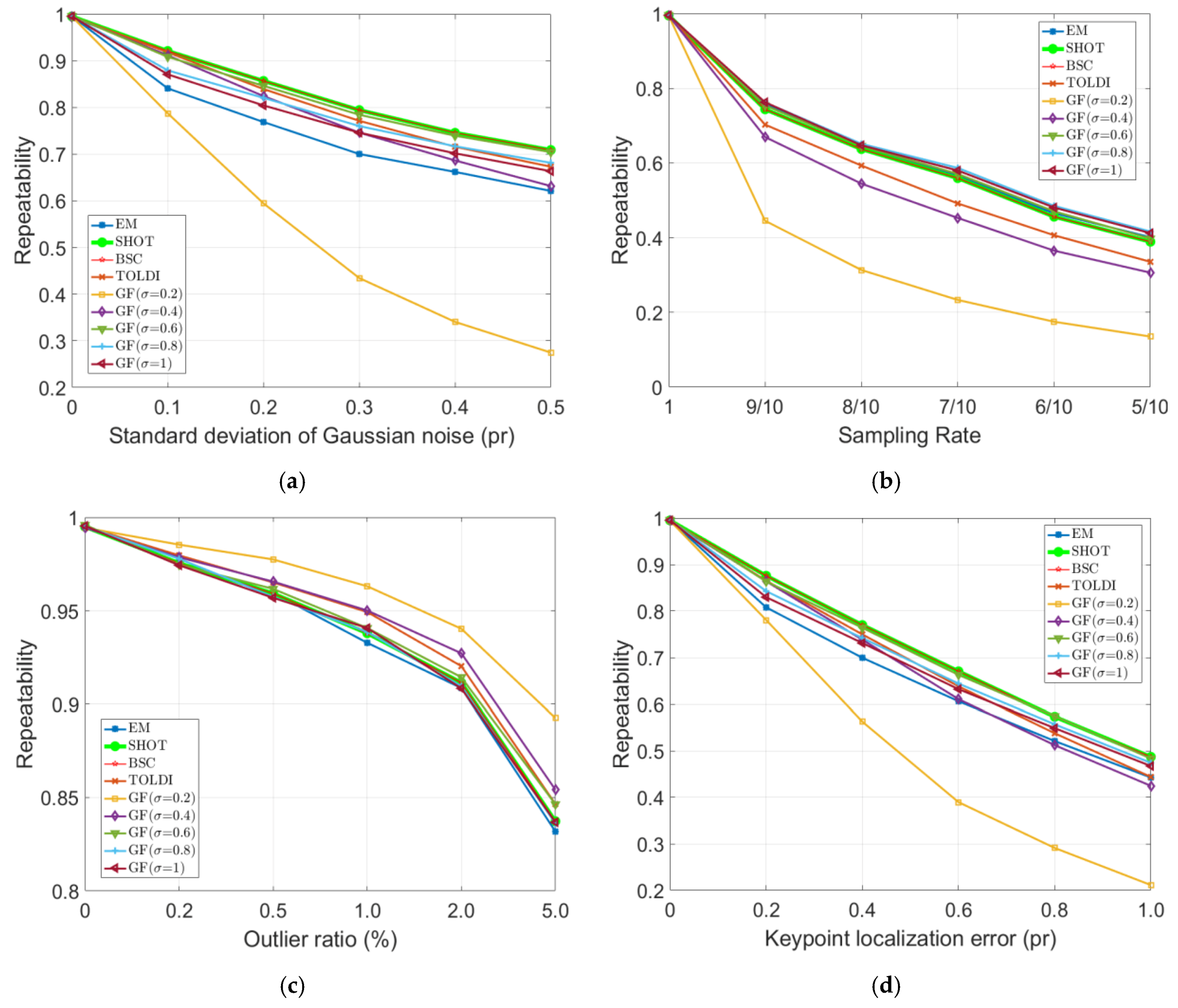
In the experiments, the Retrieval dataset is applied. The four kinds of nuisances are respectively injected into the 6 noise-free scenes. The standard deviation of Gaussian noise is set as 0.1pr, 0.2pr, 0.3pr, 0.4pr, and 0.5pr to create noisy point clouds. The sampling rate is set as 9/10, 8/10, 7/10, 6/10, and 5/10 to simulate point density variation. The outlier ratio is set as 0.2%, 0.5%, 1%, 2%, and 5% to extract some points. These points are moved along their normal vectors by a magnitude of $0.5\times R$ to create outliers. The Gaussian noise with a standard deviation of 0.2pr, 0.4pr, 0.6pr, 0.8pr, and 1pr is added to the scene keypoints to simulate keypoint localization error. The experimental results are illustrated in Figure 4.

As shown in Figure 4, for different nuisances, the best method is different. In terms of robustness to noise and keypoint localization error (Figure 4a,d), GF($\sigma =0.6$), SHOT, and BSC achieve the best performance. It indicates that the contributions of distant points should be controlled properly for the two nuisances. Both contributing too many and too little will degrade the robustness of the LRF. In terms of robustness to point density variation (Figure 4b), GF($\sigma =0.8$), GF($\sigma =1$), and EM are the best methods. Therefore, the contributions of the distant points ought to be increased for point density variation. In terms of robustness to outliers (Figure 4c), GF($\sigma =0.2$) is the best method. This indicates that the contributions of the distant points should be weakened for outliers. This conclusion is just opposite to that drawn in reference [20]. The experiments of reference [20] were performed on the datasets with noise. Their conclusion is probably unreliable because the applied datasets are not only affected by outliers.

Based on the experimental results in Section 4.2 and Section 4.3, we can conclude that when the weights of the distant points are too large (e.g., EM), the LRF is susceptible to occlusion, clutter, missing regions, noise, outliers, and keypoint localization error. However, when the weights of the distant points are too small (e.g., GF($\sigma =0.2$)), the LRF is sensitive to noise, point density variation, and keypoint localization error.

4.4. Comparison of Weights

In order to further compare the five weighting methods, we depicte the weight values of the five weighting methods, which are shown in Figure 5. Because the weights are relative quantities, we need to normalize the weights, i.e., all the weights are divided by the maximum weight for each method.

From Figure 5b, we can easily know the contributions of the neighboring points with different distances to the covariance matrix in each method. The normalized weights of SHOT are absolutely the same as that of BSC. This explains why the two methods always get the same performance in the experiments. Therefore, we can also infer that the weighting method ($w_{q_i}={(\frac{R-\Vert {\mathit{q}}_i-\mathit{p}\Vert }{R})}^2$) is equivalent to TOLDI. We can also see that EM and TOLDI are two relatively extreme methods. This explains why the two methods always achieve relatively poor performance on some datasets. Certainly, GF($\sigma =0.2$) is also an extreme method, so the method always obtains the poorest performance.

4.5. Performance Summary and Suggestions

We have presented the comprehensive performance of the LRF obtained by the five weighting methods. Several observations can be given. (1) The weighting methods lack universality to different data modalities. For example, GF($\sigma =0.4$) and TOLDI achieve good performance on the Laser Scanner and LiDAR Registration datasets but poor performance on the Kinect and Kinect Registration datasets. GF($\sigma =0.8$) behaves well on the Retrieval dataset but performs poorly on the Laser Scanner dataset. (2) The application scenario has little influence on the performance of the weighting method because, for different application scenarios with the same data modality, the most suitable method is basically the same. For instance, the Laser Scanner dataset is created for object recognition, and the LiDAR Registration dataset is created for 3D registration. GF($\sigma =0.4$) and TOLDI obtain the best performance on both of them. The Kinect dataset is acquired for object recognition, and the Kinect Registration dataset is acquired for 3D registration. GF($\sigma =0.8$) and EM are the superior methods on both of them. (3) The weighting method is always designed to reduce the contributions of the distant points for improving the robustness to shape incompleteness. However, this fails on some datasets such as the Kinect and Kinect Registration datasets. Even the occlusion, clutter, and missing regions are present, EM and GF($\sigma =1$) are the best methods. Because the point density variation is obvious in the two datasets, the contributions of the distant points should be enhanced, as shown in Figure 4b. (4) The weights of the distant points can be adjusted by varying the value of $\sigma$ in the GF method. We can always find a proper value of $\sigma$ for different data modalities to get a good performance. From this point of view, the GF is a generalized method, and therefore we suggest using this method to replace all the other methods. The value of $\sigma$ can be determined according to the descriptor matching performance to get the robustness to noise and keypoint localization error, as used in many papers. Then, if shape incompleteness is present, the value of $\sigma$ needs to be reduced properly to get a balanced robustness to noise, keypoint localization error, and shape incompleteness. It is worth noting that the value of $\sigma$ can also be set as 0.3, 0.5, 0.7, 0.9, 1.1, and bigger values. Better performance may be obtained than that presented in the above experiments. In addition, finding a method to adaptively determine the value of $\sigma$ for each keypoint is also desired. (5) No method is always suitable for different support radii. As shown in Figure 3d, when the support radius is 15pr, the repeatability of the LRF is the highest. Therefore, we suggest that the support radius is set as 15pr. (6) As shown in Figure 3a–c, with the increase of the degree of shape incompleteness, the ranking of the methods is unchanged on the whole. Hence, the weighting method should be mainly designed to get robustness to other nuisances, and then it should be properly adjusted to get the robustness to shape incompleteness. (7) Another weighting method to improve the robustness against point density variation is necessary because the ranking of the method under the nuisance is different from that under noise and keypoint localization error, as shown in Figure 4. (8) Similarly, a mechanism should be applied to detect and eliminate outliers.

5. Conclusions

We have conducted a comprehensive performance evaluation of five state-of-the-art weighting methods on six benchmark datasets, which refer to different data modalities and different application scenarios. The performance of the LRF is assessed under different kinds of nuisances, including occlusion, clutter, partial overlap, varying support radii, Gaussian noise, shot noise, point density variation, and keypoint localization error. Through our experiments, the five weighting methods are compared, and a qualitative assessment is provided. The performance summary and suggestions are also presented as a valuable reference for the design of a new LRF method.

References

1. Guo, Y.; Sohel, F.; Bennamoun, M.; Lu, M.; Wan, J. Rotational projection statistics for 3D local surface description and object recognition. Int. J. Comput. Vis. 2013, 105, 63–86. [Google Scholar] [CrossRef] [Green Version]
2. Johnson, A.E.; Hebert, M. Using spin images for efficient object recognition in cluttered 3D scenes. IEEE Trans. Pattern Anal. Mach. Intell. 1999, 21, 433–449. [Google Scholar] [CrossRef] [Green Version]
3. Lu, M.; Guo, Y.; Zhang, J.; Ma, Y.; Lei, Y. Recognizing objects in 3D point clouds with multi-scale local features. Sensors 2014, 14, 24156–24173. [Google Scholar] [CrossRef] [PubMed] [Green Version]
4. Tateno, K.; Tombari, F.; Navab, N. When 2.5D is not enough: Simultaneous reconstruction, segmentation and recognition on dense SLAM. In Proceedings of the 2016 IEEE International Conference on Robotics and Automation (ICRA), Stockholm, Sweden, 16–21 May 2016. [Google Scholar]
5. Dong, Z.; Yang, B.; Liang, F.; Huang, R.; Scherer, S. Hierarchical registration of unordered TLS point clouds based on binary shape context descriptor. ISPRS J. Photogramm. Remote Sens. 2018, 144, 61–79. [Google Scholar] [CrossRef]
6. Guo, Y.; Sohel, F.; Bennamoun, M.; Wan, J.; Lu, M. An accurate and robust range image registration algorithm for 3D object modeling. IEEE Trans. Multimed. 2014, 16, 1377–1390. [Google Scholar] [CrossRef]
7. Gao, Y.; Dai, Q. View-based 3-D object retrieval: Challenges and approaches. IEEE Multimed. 2014, 21, 52–57. [Google Scholar] [CrossRef]
8. Salti, S.; Tombari, F.; Di Stefano, L. On the use of implicit shape models for recognition of object categories in 3D data. In Asian Conference on Computer Vision; Springer: Berlin, Heidelberg, 2011; Volume 6494, pp. 653–666. [Google Scholar]
9. Guo, Y.; Bennamoun, M.; Sohel, F.; Lu, M.; Wan, J. 3D Object recognition in cluttered scenes with local surface features: A survey. IEEE Trans. Pattern Anal. Mach. Intell 2014, 36, 2270–2287. [Google Scholar] [CrossRef]
10. Yamany, S.M.; Farag, A.A. Free-form surface registration using surface signatures. In Proceedings of the 7th IEEE International Conference on Computer Vision, Kerkyra, Greece, 20–27 September 1999; Volume 2, pp. 1098–1104. [Google Scholar]
11. Yang, J.; Cao, Z.; Zhang, Q. A fast and robust local descriptor for 3d point cloud registration. Inf. Sci. 2016, 346, 163–179. [Google Scholar] [CrossRef]
12. Albarelli, A.; Rodolà, E.; Torsello, A. Fast and accurate surface alignment through an isometry-enforcing game. Pattern Recognit. 2015, 48, 2209–2226. [Google Scholar] [CrossRef]
13. Tombari, F.; Salti, S.; Di Stefano, L. Unique signatures of histograms for local surface description. In European Conference on Computer Vision; Springer: Berlin, Heidelberg, 2010; pp. 356–369. [Google Scholar]
14. Guo, Y.; Sohel, F.; Bennamoun, M.; Wan, J.; Lu, M. A novel local surface for 3D object recognition under clutter and occlusion. Inf. Sci. 2015, 293, 196–213. [Google Scholar] [CrossRef]
15. Yang, J.; Zhang, Q.; Xian, K.; Xiao, Y.; Cao, Z. Rotational contour signatures for both real-valued and binary feature representations of 3D local shape. Comput. Vis. Image Understand. 2017, 160, 133–147. [Google Scholar] [CrossRef]
16. Johnson, A.E.; Hebert, M. Surface matching for object recognition in complex three-dimensional scenes. Image Vis. Comput. 1998, 16, 635–651. [Google Scholar] [CrossRef]
17. Rusu, R.B.; Blodow, N.; Beetz, M. Fast point feature histograms (FPFH) for 3d registration. In Proceedings of the IEEE International Conference on Robotics and Automation, Kobe, Japan, 12–17 May 2009; pp. 3212–3217. [Google Scholar]
18. Yang, J.; Zhang, Q.; Xiao, Y.; Cao, Z. TOLDI: An effective and robust approach for 3D local shape description. Pattern Recognit. 2017, 65, 175–187. [Google Scholar] [CrossRef]
19. Guo, Y.; Bennamoun, M.; Sohel, F.; Lu, M.; Wan, J.; Kwok, N.M. A comprehensive performance evaluation of 3d local feature descriptors. Int. J. Comput. Vis. 2016, 116, 66–89. [Google Scholar] [CrossRef]
20. Yang, J.; Xiao, Y.; Cao, Z. Toward the repeatability and robustness of the local reference frame for 3D shape matching: An evaluation. IEEE Trans. Image Process. 2018, 27, 3766–3781. [Google Scholar] [CrossRef]
21. Guo, Y.; Bennamoun, M.; Sohel, F.; Lu, M.; Wan, J. An integrated framework for 3-D modeling, object detection, and pose estimation from point-clouds. IEEE Trans. Instrum. Meas. 2015, 64, 683–693. [Google Scholar]
22. Tombari, F.; Di Stefano, L. Object recognition in 3D scenes with occlusions and clutter by Hough voting. In Proceedings of the 2010 Fourth Pacific-Rim Symposium on Image and Video Technology, Singapore, 14–17 November 2010; pp. 349–355. [Google Scholar]
23. Petrelli, A.; Di Stefano, L. Pairwise registration by local orientation cues. Comput. Graph. Forum 2016, 35, 59–72. [Google Scholar] [CrossRef]
24. Dong, Z.; Yang, B.; Liu, Y.; Liang, F.; Li, B.; Zang, Y. A novel binary shape context for 3D local surface description. ISPRS J. Photogramm. Remote Sens. 2017, 130, 431–452. [Google Scholar] [CrossRef]
25. Petrelli, A.; Di Stefano, L. A repeatable and efficient canonical reference for surface matching. In Proceedings of the 2012 2nd International Conference on 3D Imaging, Modeling, Processing, Visualization & Transmission, Zurich, Switzerland, 13–15 October 2012; pp. 403–410. [Google Scholar]
26. Novatnack, J.; Nishino, K. Scale-dependent/invariant local 3D shape descriptors for fully automatic registration of multiple sets of range images. In European Conference on Computer Vision; Springer: Berlin, Heidelberg, 2008; pp. 440–453. [Google Scholar]
27. Levin, D. Mesh-Independent surface interpolation. Geometric Modeling for Scientific Visualization. Mathematics and Visualization; Springer: Berlin, Heidelberg, 2004; pp. 37–49. [Google Scholar]
28. Tombari, F.; Salti, S.; Di Stefano, L. Performance evaluation of 3D keypoint detectors. Int. J. Comput. Vis. 2013, 102, 198–220. [Google Scholar] [CrossRef]
29. Mian, A.; Bennamoun, M.; Owens, R. On the repeatability and quality of keypoints for local feature-based 3D object retrieval from cluttered scenes. Int. J. Comput. Vis. 2010, 89, 348–361. [Google Scholar] [CrossRef] [Green Version]
30. Mian, A.S.; Bennamoun, M.; Owens, R. Three-dimensional model based object recognition and segmentation in cluttered scenes. IEEE Trans. Pattern Anal. Mach. Intell. 2006, 28, 1584–1601. [Google Scholar] [CrossRef] [PubMed] [Green Version]
31. Kammerl, J.; Blodow, N.; Rusu, R.B.; Gedikli, S.; Beetz, M.; Steinbach, E. Real-time compression of point cloud streams. In Proceedings of the 2012 IEEE International Conference on Robotics and Automation, Saint Paul, MN, USA, 14–18 May 2012; pp. 778–785. [Google Scholar]
Figure 1. The process diagram of building a local reference frame.
Applsci 10 03223 g001
Figure 2. Experimental datasets. (a) Retrieval, (b) Laser Scanner, (c) Kinect, (d) Space Time, (e) LiDAR Registration, and (f) Kinect Registration. A model and a scene (from left to right) are presented as examples for each dataset.
Applsci 10 03223 g002
Figure 3. The repeatability of LRF obtained by the five weighting methods with respect to four kinds of nuisances, including (a) occlusion, (b) clutter, (c) partial overlap, and (d) varying support radii.
Applsci 10 03223 g003
Figure 4. The repeatability of LRF obtained by the five weighting methods with respect to four kinds of nuisances, including (a) Gaussian noise, (b) point density variation, (c) shot noise, and (d) keypoint localization error.
Applsci 10 03223 g004
Figure 5. The weights calculated by the five weighting methods, including (a) weights, (b) normalized weights.
Applsci 10 03223 g005