Article

A Power Performance Online Assessment Method of a Wind Turbine Based on the Probabilistic Area Metric

1
School of Mechanical Engineering, Hunan University of Science and Technology, Xiangtan 411201, China
2
XEMC Wind Power Co., Ltd., Xiangtan 411102, China
*
Author to whom correspondence should be addressed.
Appl. Sci. 2020, 10(9), 3268; https://doi.org/10.3390/app10093268
Submission received: 18 March 2020 / Revised: 30 April 2020 / Accepted: 2 May 2020 / Published: 8 May 2020
(This article belongs to the Special Issue Wind Power Technologies)

Abstract

:
This paper presents an approach for creating online assessment power curves by calculating the variations between the baseline and actual power curves. The actual power curve is divided into two regions based on the operation rules of a wind turbine, and the regions are individually assessed. The raw data are filtered using the control command, and outliers are detected using the density-based spatial clustering of applications with noise clustering method. The probabilistic area metric is applied to quantify the variations of the two power curves in the two regions. Based on this result, the variation in the power curves can be calculated, and the results can be used to dynamically evaluate the power performance of a wind turbine. The proposed method is verified against the derivation of secondary principal component method and traditional statistical methods. The potential applications of the proposed method in wind turbine maintenance activities are discussed.

1. Introduction

Wind energy is essential to the satisfaction of electrical power demands in an environmentally sustainable manner. With the increase in installed wind power capacity, the operation and maintenance (O&M) costs of wind turbines are gradually increasing. Research has shown that the use of a supervisory control and data acquisition (SCADA) system is an economical and effective method for identifying early signs of failure and performance issues; thus, such systems have been widely installed in large-scale wind turbines. Using the SCADA system, large quantities of environmental data and equipment status data are stored. By mining these SCADA data, several investigations can be carried out, such as for condition monitoring [1,2,3], fault diagnosis [4,5], ageing [6,7] and reliability assessment of wind turbines [8]. A wind turbine is a piece of equipment that generates electricity through the conversion of the kinetic energy of the wind, which automatically adjusts the operating state according to the wind speed and direction. The research and application of the real-time monitoring and fault diagnosis are important to ensure the wind turbine safety and save O&M costs [9,10]. The electricity generation performance of wind turbines is an important index that manufacturers, wind farm operators, investors and grid operators consider.
The power curve is commonly used to monitor wind turbine power performance, as it is an important indicator that reflects the electricity generation performance. By monitoring the variation in the power curve, the operating power performance of wind turbines can be assessed, and problems can be identified [11]. Therefore, it is necessary to define a baseline power curve that represents the optimal power performance of the wind turbine. This reference curve is either constructed by using the measured wind-power data or provided by the wind turbine manufacturers [11,12]. The actual power curve generated by SCADA data can be compared with this baseline curve, and the deviation between the two curves can reflect variations in power performance. This deviation is often represented as a health value (HV) or confidence value [13,14]. Further trend analysis on the gradual change of the health value will help to identify signs of performance degradation, performance optimization opportunities, incipient fault detection, and so on. Due to the highly dynamic and stochastic operating conditions, the wind-power data from the SCADA system contain a large quantity of abnormal data because of underperformance, changes in wind resources or equipment failure/anomalies such as pitch system faults and ice on the blade [15,16]. Therefore, the efficient and objective calculation of the health value is key to power performance assessment.
At present, a considerable number of methods are used to calculate the health value. Some of these approaches first model the actual power curves and then analyze the deviations between the baseline power curve and the actual power curve. Such approaches are called parametric evaluation methods. Kusiak et al. [17] constructed parametric models of the power curve with a logistic function to monitor wind turbine performance. Other parametric modelling methods have been presented, such as the bin method [18], the evaluation method [19], the Gaussian process [20,21], fuzzy clustering [22], the copulas function [23], the Gaussian mixture model and the neural network [24]. Based on the parametric model, performance assessment methods that use the baseline power curve for comparison were presented. These comparison methods included minimum quantization error, Euclidean distance and residue analysis. A comparative study of wind turbine performance assessment based on three typical parametric evaluation methods was carried out in reference [25]. The results indicated that the Gaussian mixture model-L2 distance (GMM-L2) method is suitable for degradation modelling and performance prediction. However, parametric evaluation methods involve model selection, parameter estimation, error modelling and algorithm convergence; thus, these methods require human intervention to acquire the best parametric model, which is mainly used for offline data analysis. To achieve online wind turbine assessment, there are many problems to overcome. To avoid modelling problems, nonparametric assessment methods that directly assess the actual wind-power data and the baseline wind-power data were proposed [26,27,28], the derivation of secondary principal component (PCA2-Dev) method is a representative method [27]. PCA2-Dev reduced the dimensionality of wind-power data via principal analysis and selected power data as the main evaluation data. The deviations were calculated by using the ratio of the standard deviations of the baseline power data and the actual power data. However, PCA2-Dev could assess only quasilinear wind-power data and could not be used with rated power data. However, the wind turbine maximized its power output in the rated power region; thus, performance fluctuation this region would affect the economic benefit of wind farms. Therefore, SCADA data in the rated power region need to be assessed.
In this paper, a novel nonparametric assessment method is developed based on the probabilistic area metric that can compute the health value of the actual wind-power data by locating either the quasilinear region or the rated power region and achieve online assessment in real time. The presented method is compared with the PCA2-Dev method and traditional statistical methods. The results show that the proposed method is simple and effective. In addition, because the probabilistic area metric is used in the proposed method for direct derivation, an iterative process is not required, and convergence does not need to be considered. The assessment result shows that the power performance variation is stable; thus, this result appropriate for prediction analysis. In summary, the key scientific contributions of this paper are as follows:
  • The probabilistic area metric is used to evaluate the deviations of the probabilistic models of two datasets. In other words, the datasets are transformed into probabilistic models instead of means or variances, and the deviations of the probabilistic models are calculated. The area metric has an obvious advantage in dynamic and stochastic SCADA data mining analysis.
  • The assessment method combines physical model analysis and data mining techniques. The assessment result is statistically significant, and it has physical significance and is easy for engineers to understand.
The rest of this paper is organized as follows. Section 2 introduces the basic theory of power curves and establishes the objective of the current study. Section 3 explains the data preprocessing method, the principle of selecting the baseline data, the health value based on the probabilistic area metric and the calculation flow. In Section 4, the proposed method is compared with the PCA2-dev method and the traditional statistical approach. Section 5 discusses the application of the present method in performance optimization, degradation analysis and condition pre-warnings. Section 6 summarizes the study.

2. Problem Definition

2.1. Power Curves

A wind turbine power curve depicts the relationship between the hub wind speed and output power, and it is an important index for evaluating the wind turbine performance. As shown in Figure 1, the power curve can be divided into four regions according to the operational features. In Region A, where the wind speed is lower than the cut-in speed v in , no electric power generation occurs. In Region B, the wind speed v [ v in , v rated ] , and v rated is rated wind speed. The maximum wind power tracking can be attained. According to Betz’s Law, the theoretical maximum utilized wind power is called the Betz theoretical limit value, the coefficient of which is 0.593. To produce maximum power, several types of control strategies are applied, such as pitch angle control, generator torque control and yaw control, to approximate the Betz curve as much as possible. In Region C, where in which the wind speed v [ v rated , v out ] , the wind turbine remains at the rated power. As the wind speed increases, the tip speed ratio decreases more rapidly than that in the constant rotation region, and the wind turbine runs at a constant power with a smaller wind turbine power coefficient CP. In Region D, where the wind speed is faster than the cut-out speed, the pitch angle is adjusted to 90°; consequently, the turbine blades stop rotating, and wind power is no longer generated. By analyzing the operational features of the power curve, Regions B and C can be noted as the main working regions, and these regions are selected as the research objects for assessing the operation condition of a wind turbine. For convenience, Region B is called the maximum wind power tracking region (MWPTR), while Region C is called as the rated power output region (RPOR).

2.2. Problem Statement and Purpose of Assessment

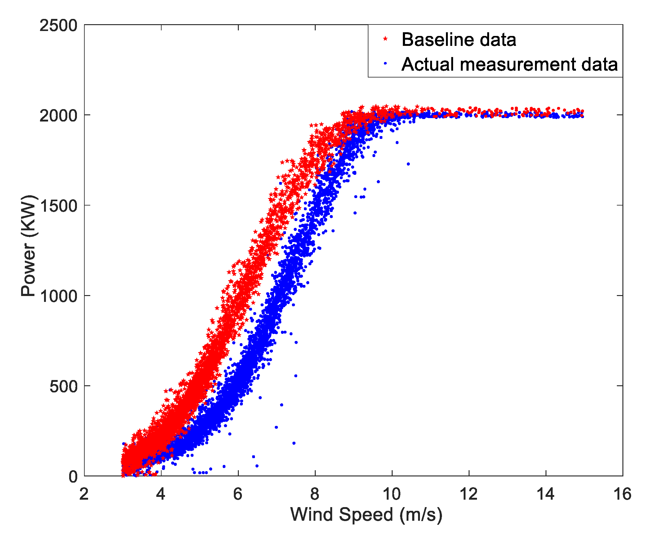
The ageing of components or change in wind resources due to long-term service could lead to output power fluctuations of the wind turbine. As shown in Figure 2, an obvious deviation exists between the actual measurement data and the baseline data in the MWPTR. Therefore, on-line performance assessment of a wind turbine can be realized by quantifying the deviations of power curves and analyzing the change trends to provide a reference for operations and maintenance decision-making.
This paper proposes a power performance assessment method by mining 10-min SCADA data; this method could prove to be a useful tool for operation and maintenance staff when assessing the overall performance of a wind turbine and to making maintenance plans. The performance assessment of wind turbines based on power curve monitoring requires a set of complete dataset in the MWPTR and RPOR, which is used to determine the change trend of the wind turbine. The wind speed and output power have different mapping relations in the MWPTR and RPOR; therefore, the assessment method must consider these distinctions in different wind speed regions. In particular, the control objective of MWPTR is to capture the maximum wind power capture, while RPOR is oriented to achieve as much output power as possible while maintaining a stable output power. Based on the analysis derived from Figure 2, the proposed assessment method must possess the following features:
(1)
The evaluation results must accurately indicate the variations between the actual power curve and the baseline power curve.
(2)
The method must be robust and unaffected by the presence of outliers.
(3)
The method must be able to be implemented simply, and the assessment results must be easy to understand for engineers to understand.
(4)
A stable trend of power performance changes must be acquired, as this trend can be used for prediction analysis.

3. Power Performance Assessment Methodology

3.1. Baseline Data Selection

Baseline data are obtained from the operation data of a real wind turbine; they represent the optimal operation state of the turbine and are used to produce the reference power curve for the condition assessment. In this study, the baseline data were selected from an optimally performing wind turbine; the data were verified and pertained to a continuous period. To select the baseline data, both the wind resource and operating condition of the wind turbine should be taken into consideration. In terms of the wind resource, it is ideal to select wind–power operation data in an abundant wind resource period, to ensure that complete assessment information in the region from cut-in wind speed to rated wind speed can be obtained. Information pertaining to operation and maintenance, such as repair reports and downtime, can be used to evaluate the operational condition. Finally, using theoretical and experimental analyses, a comparative analysis of these preselected baseline data can be conducted to acquire the optimal wind speed and power data of the entire wind farm, which is defined as the baseline data.

3.2. Preprocessing

Based on the control principle of the wind turbine, SCADA data can be filtered using the following steps: (1) Filter out data for which power P = 0. (2) Eliminate data for which the wind speeds are less than vin or greater than vout. (3) Filter out artificially limited electricity data by the control command, such as the limit value of the wind turbine power and generator power. (4) Determine the wind speed and power data in the MWPTR and RPOR according to v in , v out and v rated . In other words, v in < v < v rated correspond to the MWPTR, while v rated < v < v out correspond to the RPOR.
SCADA data including numerous abnormal data such as sensor abnormality and icing are identified using the density-based spatial clustering of applications with noise (DBSCAN) clustering method [29]. The DBSCAN clustering method, a typical clustering method based on density, can identify a cluster by setting a density threshold. This clustering algorithm has two key parameters—Eps and Minpts. Eps represents the radius of cluster, and Minpts is the number of neighbors within the cluster. With reference to [30,31], Minpts is set to 4 in this study, and Eps is calculated using the following equation:
Eps = ( V × MinPts × γ ( 0.5 × n + 1 ) m π n ) 1 n
where m denotes the number of objects in the experimental data set, n is the dimensionality of the experimental space, γ ( · ) is the factorial function, and V is the volume of the experimental space formed by m objects:
V = i = 1 n { max ( x i ) min ( x i ) }
where max ( · ) is the largest value function, min ( · ) is the smallest value function, x i is the i-th column data of the m-by-n experimental data matrix.

3.3. Health Value Based on the Probabilistic Area Metric

3.3.1. Health Value in the MWPTR

According to the interval size δ , the MWPTR can be divided into t intervals, and the ith wind speed interval can be expressed as [ v i m e a n δ , v i m e a n + δ ] . The assessment data can be expressed as { ( v 1 , P 1 ) , ( v 2 , P 1 ) , , ( v n , P n ) } , in which the points falling within the ith wind speed interval are expressed as ( v i , j , P i , j ) ; here, the first subscript denotes the interval number, and the second subscript indicates the number of points in the interval. Similarly, the baseline data are divided into t intervals, in which each interval point set is { C 1 0 , C 2 0 , , C n 0 } , where C i 0 corresponds to a point set ( v i , j 0 , P i , j 0 ) within the ith interval. The empirical cumulative distributive function (ECDF) in the ith interval can be calculated using:
F i 0 ( P ) = 1 m j = 1 m I [ P i , j 0 P ]
F i ( P ) = 1 k j = 1 k I [ P i , j P ]
where I is the indicator function [32]. Next, the deviation M i between the baseline data in the ith interval and the actual measurement data can be mathematically expressed as:
M i = 1 P ¯ i 0 | F i 0 ( P ) F i ( P ) | d P
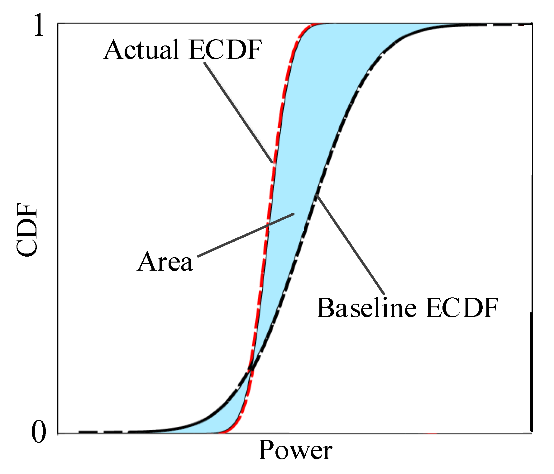
where P ¯ i 0 is the mean value of power in the ith interval, M i is the ratio of the probabilistic area and P ¯ i 0 . To explain the probabilistic area metric (PAM), the actual ECDF and baseline ECDF are shown in Figure 3. There is a contact point of two ECDF curves. The probabilistic area is cyan region of two ECDF curves, which can be calculated by the integral method in the Equation (5). It is possible that actual ECDF and baseline ECDF have no contact point. In other words, the actual ECDF is always above or under the baseline ECDF. The probabilistic area is also computed by the Equation (5).
After calculating the deviations in t intervals, the standard power curve is used to compound the overall variations. Assuming the standard power curve can be expressed as P = g ( v ) , where v is the wind speed, P is the power and g ( ) is the standard power curve function. The power of the mean point in the ith speed interval should be:
P i m e a n = g ( v i m e a n )
where v i m e a n is mean of the ith wind speed interval, P i m e a n is the power of the standard power curve. In the i interval, the weighting value κ i is calculated by:
κ i = P i m e a n i = 1 t P i m e a n
The HV in the MWPTR is:
γ MWPTR = κ 1 M 1 + κ 2 M 2 + + κ t M t
In the MWPTR, the control objective of wind turbine is to track the maximum wind power. γ MWPTR represents the derivation that the actual power data from the baseline data. The HV with an approximate zero value means that the individual wind turbine is close to the optimal power performance. Conversely, a higher HV represents a poorer health condition. The reasons may be equipment fault, machine degradation, weather and so on. By analyzing γ MWPTR and its change trend, it is beneficial to condition assessment and monitoring.

3.3.2. Health Value in the RPOR

The theoretical power curve in the RPOR is a horizontal line equal to the rated power. The actual wind speed and power points in the RPOR are assessed together. Using the rated wind speed and cut-out wind speed, the dataset in the RPOR can be selected and defined as C rated , and the wind speed and power data can be expressed as ( v i r , P i r ) ( i = 1 , 2 , , s ) . The baseline data in the RPOR are defined as C rated B , and the wind speed and power data can be expressed as ( v i 0 , r , P i 0 , r ) ( i = 1 , 2 , , s 1 ) . The health value can be calculated using:
γ rated = | F 0 , r ( P ) F r ( P ) | d ( P )
where
F 0 , r ( P ) = 1 s 1 j = 1 s 1 I [ P j 0 , r P ]
F r ( P ) = 1 s j = 1 s I [ P j r P ]
where γ rated is the HV in the RPOR. A small γ rated means the well health condition. Conversely, γ rated with a higher value represents the poorer health condition.

3.4. Calculation Flowchart

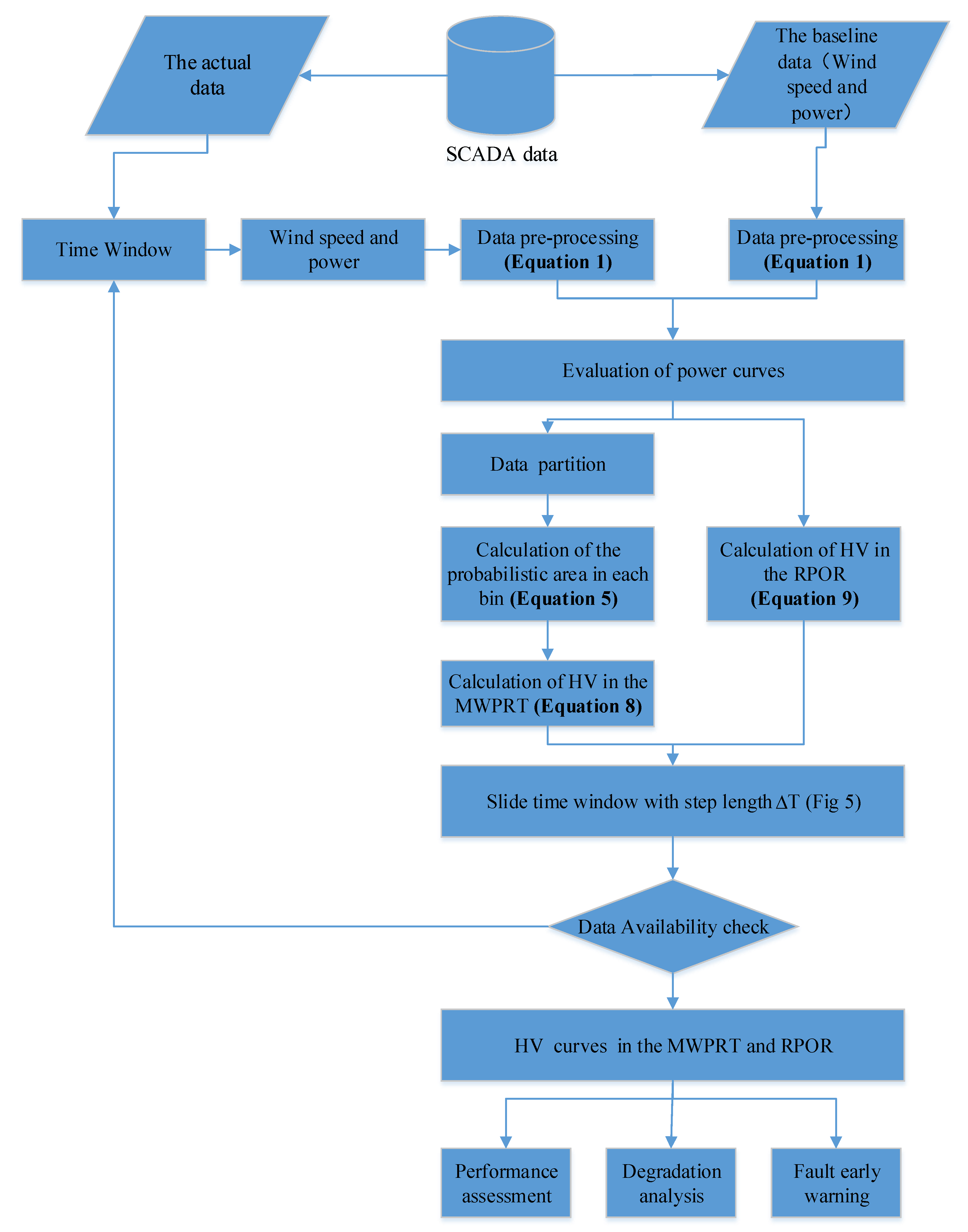
The assessment flowchart of the power performance based on the PAM is shown in Figure 4. First, the useful parameters are collected from the SCADA system, including the nacelle wind speed, power, hub rotational speed, and electricity limitation command. Next, the time window length T and slide step length ΔT need to be determined, as shown in Figure 5. The window length T is related to the quality of data of the considered wind farm, and these data are of a size similar to the baseline data used in this study. ΔT is determined according to the assessment needs. SCADA data of 10 min are taken as an example; T pertains to 20 days, and the wind speed and power data pertain to 2280 days. If we set ΔT as the data obtained in a day, then 144 data points should be collected. However, due to data loss, downtime data and abnormal data, the actual number of T is less than 2280, and ΔT is less than 144. Therefore, to avoid the impact of insufficient data, T and ΔT are determined by referring to the preprocessed data. The corresponding assessment result γ index is thus not the result of equal time intervals, as shown in Figure 5.
The baseline data and actual data are both divided into MWPTR and RPOR. The DBSCAN method is used to preprocess the data, in which Eps_opt is calculated using Equation (1). Next, the wind speed and power data in the MWPTR and RPOR are evaluated using the methods proposed in Section 3.3.1 and Section 3.3.2, respectively. The values of γ MWPTR and γ rated of the wind turbine can be computed by Equations (8) and (9). After assessing the performance of the R region, the new assessment data can be obtained by sliding the windows with step ΔT. The update method of the evaluation data is shown in Figure 5. With the same calculation process, the HV of different time windows can be obtained. For SCADA data pertaining to a long duration, two time series can be acquired, which are defined as { γ MWPTR 1 , γ MWPTR 2 , , γ MWPTR n } and { γ rated 1 , γ rated 2 , , γ rated n } . Later, through analysis of the time series of the HV, operations and maintenance activities, such as performance assessment, degradation analysis and early warning, fault detection, can be better performed.

4. Verification of Results

4.1. MWPTR Results

The SCADA data used in this study are obtained from a mountain wind farm which has 24 sets of 2 WM wind turbines. The cut-in wind speed v in is 3 m/s, the cut-out wind speed v out is 25 m/s, and the rated wind speed v rated is 11 m/s. In this study, 10 min of SCADA data are used, and the wind speed data are collected from the nacelle sensor. In addition, the SCADA data pertains to the period from 1 January 2013 and 31 December 2017. The analysis of the operation conditions of all the wind turbines in the wind farm indicated that the T01 wind turbine demonstrates relatively stable performance with fewer maintenance activities during its service. Through a comparative analysis with other wind turbines, with reference to the wind resource and maintenance records, data of the T01 wind turbine from June to July 2015 are selected as the baseline data. The length of the time window T is 4320 (30 days), and the slide step size ΔT is 432(3 days).
HV curve of the T01 wind turbine is calculated and given in Figure 6, it can be seen that a larger HV corresponds to poorer power performance. In addition, if two health values are farther from each other along the horizontal axis, there may be downtime. From Figure 6, it can be noted that HV is between 0.4 and 0.5 before Date A. During the time interval between Dates A and C, HV changes violently. During Dates C and D, the wind turbine operates in a stable manner, fluctuating only in a remarkably short interval with little downtime, which is consistent with the actual maintenance record. To clarify whether the HV can actually reflect the variations between the reference data and the actual data, the wind speed and power data of Dates A, B and C are plotted, as shown in Figure 7. From Figure 7a, it can be found that the deviation between Date A and Date C is extremely pronounced, and Point B indicates a transition from Date A to Date C. Therefore, the HV with the presented method accurately quantifies the power performance changes. More importantly, the gradual change of the HV is objectively presented. Further trend analysis will be meaningful for the turbine operation and maintenance activities.
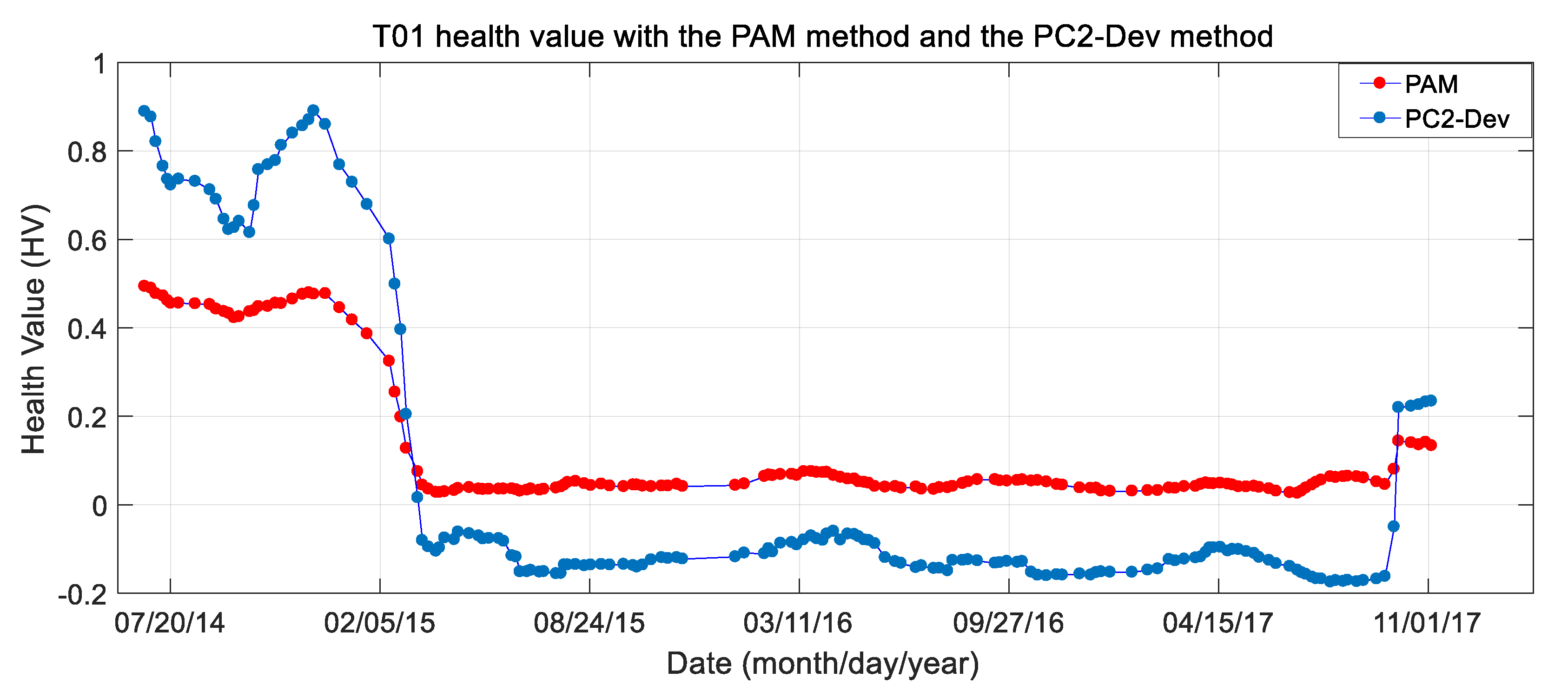
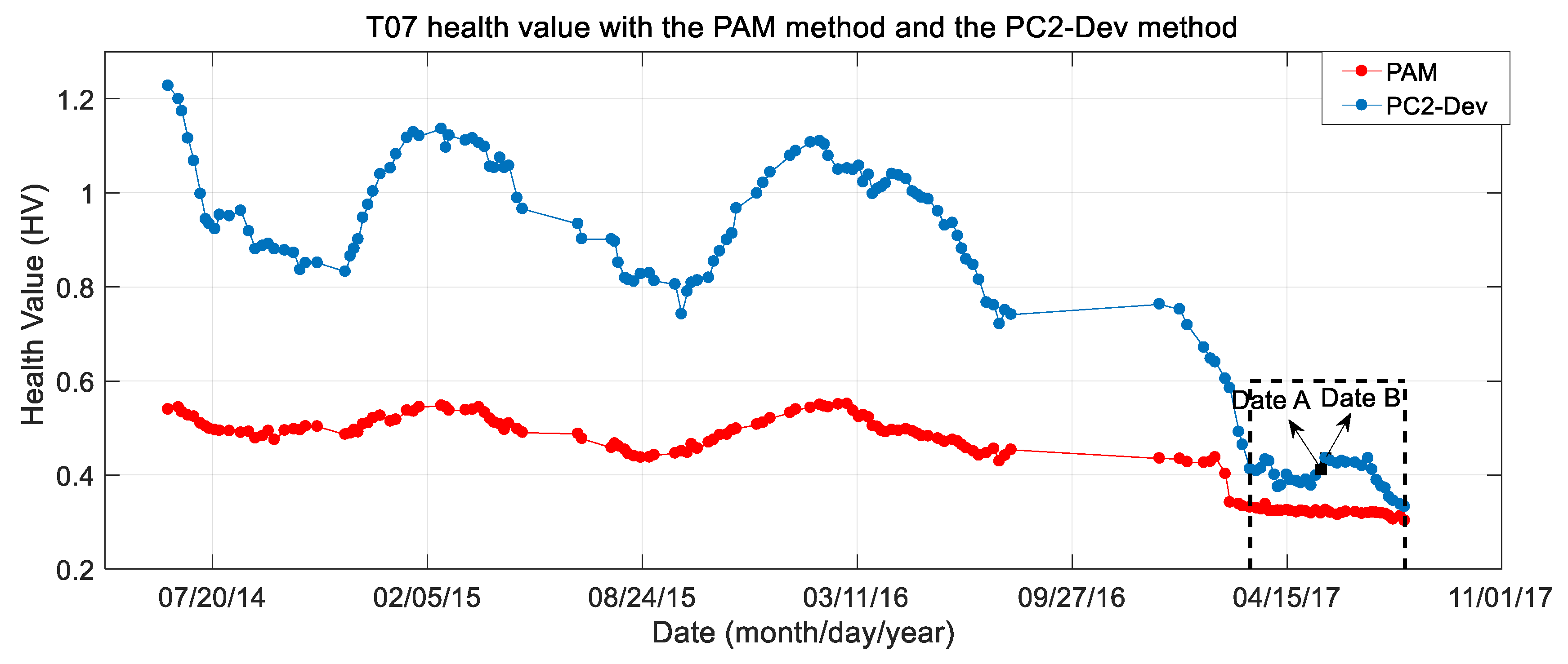
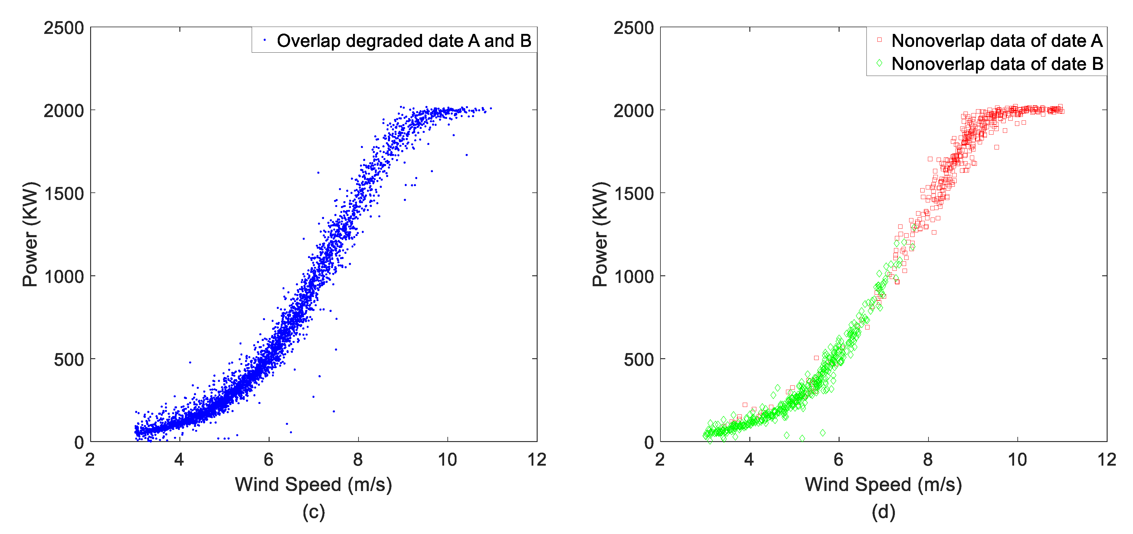
To further prove the validity of the presented method, a comparative study is performed using the PC2-Dev method [27]. T01 and T07 are both selected as research objects and analyzed using two different methods. The respective results are shown in Figure 8 and Figure 9, in which the blue and red lines respectively represent the results obtained using the PC2-Dev method and the PAM method. From Figure 8, two HV curves reflect the change trend of the actual power curve well; meanwhile, the inflection points in the two curves occur nearly simultaneously. In addition, in Figure 9, from March 2014 to January 2017, the two health value curves also demonstrate a similar trend. However, it must be noted that from January 2017 to September 2017, the HV curves obtained using the PAM method change slightly with the date while the HV curves obtained using the PC2-Dev method exhibit large fluctuations, demonstrating distinct differences. For analyzing the reason, two points with the largest changes in the PC2-Dev method are selected and named Date A and Date B; next, their data together with the baseline data are plotted, as shown in Figure 10. Figure 10a shows data of Dates A and B, as well as the baseline data. Figure 10b shows data of Dates A and B; the overlapped part is marked in blue, as shown in Figure 10c, while others are marked in different color, as shown in Figure 10d. Based on the observation from Figure 10, Dates A and B data are remarkably similar to the baseline data, both containing a large amount of overlapped information. Therefore, it can be implied that the resultant large fluctuation of curves comes from the small number of non-overlapped data. By analyzing the non-overlapped data in Figure 10d, it can be noted that the data of Date A are mainly locate in the wind speed interval [3.0, 7.0], and the data of Date B are located in the speed interval [7.0, 11.0]. The power in interval [7.0, 11.0] is greater than that in interval [3.0, 7.0]. As seen from Figure 10, data of Dates A and B are close to the baseline data, and consequently, the corresponding health values should be similar. The HV calculated using the PAM method is consistent with the actual situation; however, that obtained using the PC2-Dev method behaves in a contrasting manner. The reason for this finding is that the PC2-Dev method adopts the principal component analysis to reduce the dimensions of wind speed and power, and calculates the HV based on the variance of the actual measurement power and the baseline power data. In fact, the variance of Date B is larger than that of Date A in this case.
Consequently, in some cases, the PC2-Dev method may calculate an abnormal HV because the variance-based method cannot reflect the entire data information. The PAM method can avoid this defect because the ECDF of data is applied to quantify the variations between the data sets, which include more information than the variance of data. The above discussion indicates that although the PC2-Dev method is an effective method to assess power curves of wind turbine, it may cause false alarms in certain situations. In this regard, the PAM method can attain better results.

4.2. RPOR Results

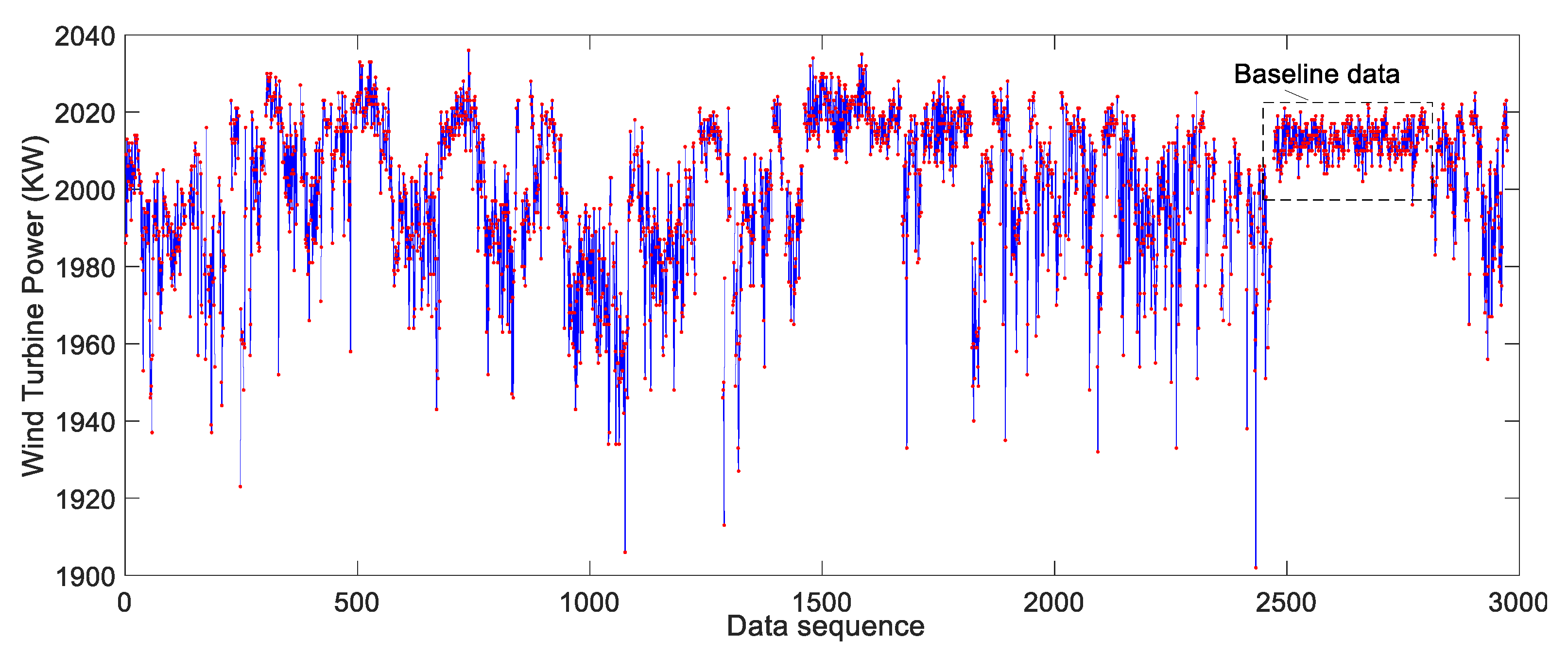
In this analysis, the rated power data of the T22 wind turbine, for the period between December 2015 and December 2017, are collected as the research object. Due to the strong turbulence of the mountain wind farm, the actual data in which the power is rated are filtered. The time series of power is plotted, as shown in Figure 11. The size of the data in the RPOR is less than 3000, and the power interval is [1900, 2040]. It could be observed that the data fluctuated considerably in the vertical direction. However, in the dashed box region, the data behaves in a stably manner, and the center value is slightly higher than the rated power value, that is, 2 MW. The theoretical analysis indicates that the output power of the wind turbine in the rated region should, in theory, stably fluctuate around the rated power value. However, the operation and maintenance companies expect to benefit more by generating more electricity under a safe level, which requires the wind turbine to operate stably with a power value slightly larger than the rated power. Based on the above analysis, the data in the dashed box are selected as the baseline data. Three hundred eight wind-power points are present in the baseline data, derived from a continuous time interval. The size of the time window T is selected to be 288, and due to inadequate data, Δ T is set as 36 to acquire a lasting change trend.
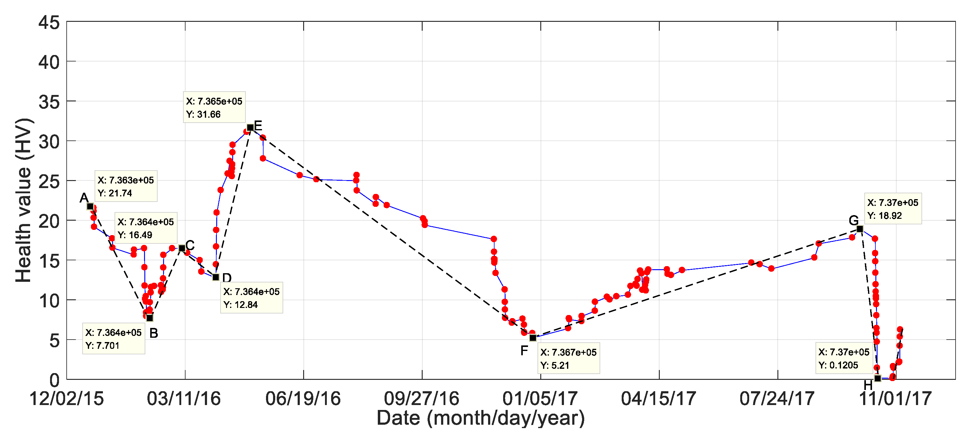
The result calculated using the PAM method is plotted, as shown in Figure 12. The red dotted line represents the HV curve. A larger HV value represents a greater deviation between the actual data and the baseline data. The two points are apart from each other with a large horizontal span, signaling a high possibility of downtime; alternatively, they might correspond to the RPOR data. The adjacent points are dense, indicating that sufficient data is available. Peak points are selected from the health value curve, labelled as Dates A–H, and they are connected using a dotted line. From Date A to Date B, the health value curve exhibits a declining trend, and from Date B to Date C, the health value curve trend is increasing. The reason was that, although the performance of the wind turbine naturally degrades as the service time increases, it can be improved through repair and maintenance. From Date C to Date H, an evident change similar to the former one is exhibited. The trend indicates that Date B and Date F do not correspond to the optimal operation state; instead, Date H has the smallest point on the curve as well as the point with the best performance point. This analysis indicates that the variation trend of the health value obtained using the PAM method is consistent with the theoretical performance change trend of repairable electromechanical equipment.
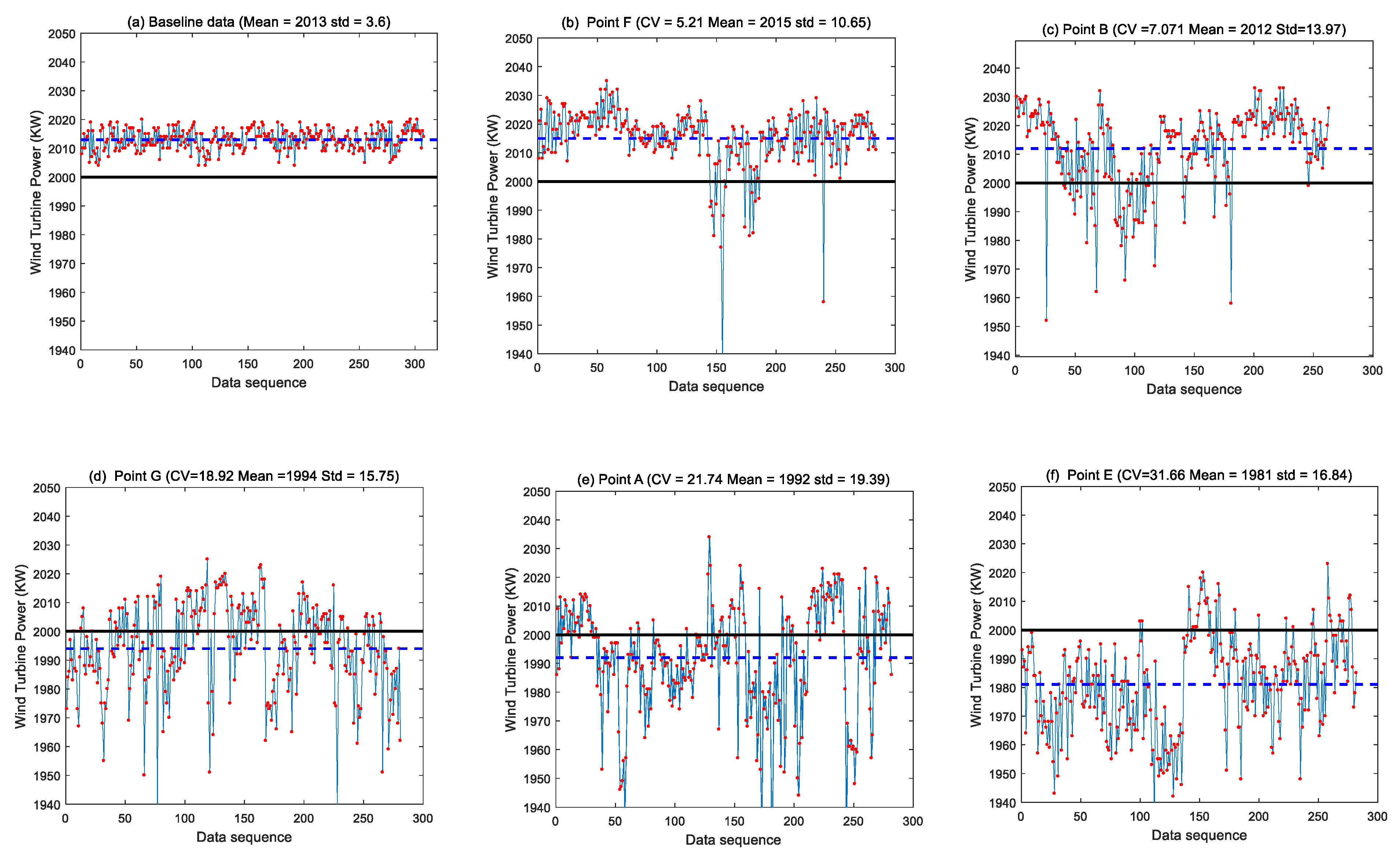
According to the research described in Section 2, the primary objective of the power curve in the MWPTR is to ensure stable operation of the wind turbine. The purpose of the PAM method is to analyze the deviation of the actual data and the baseline data. To prove whether the PAM method can efficiently calculate and describe the deviation between the two data, the mean value and variance of the baseline data at the extreme Points A, B, E, F, and G are calculated. The results are plotted in ascending order according to the HV values listed in Table 1, and the corresponding power sequence is plotted, as shown in Figure 13. Figure 13a shows that the mean value of the baseline data is 2013, the variance is 3.6, and the entire range of data points exhibits stable operation. Figure 13b shows that the HV value of node F is slightly lower than that in the baseline data, the variance is 10.65, and the values of some power points are less than 2000. B is the minimum point, slightly larger than F, with a HV value of 7.071, because its variance is larger than that of F. Figure 13c indicates that the number of points with a value lower than 2000 is smaller than that in Figure 13b. Points G, A and E are the maximum points because their mean values are smaller than the rated power and the baseline mean value, and they have large variance. The change trend can be determined from Figure 13d–f. The above analysis demonstrates that the HV value calculated using the PAM method can well reflect the deviation between the actual data and the baseline data, as well as the mean and variance of the dataset. In general, the PAM method can be an effective tool for calculating the performance change trend of wind turbines for predictive analysis.

5. Potential Implementation

5.1. Performance Optimization

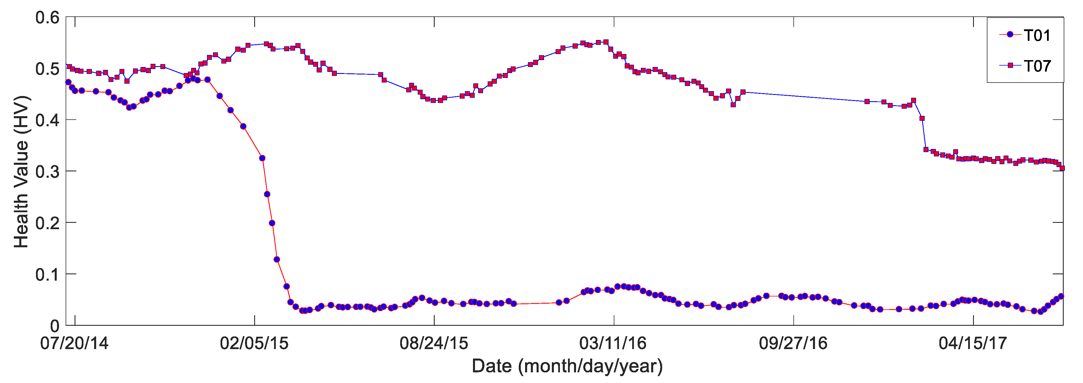
The long-term HV curves of multiple wind turbines can be determined using the PAM method, which can be used to monitor and optimize the performance of wind turbines. In Figure 14, two HV curves is shown to illustrate the performance change of the T01 and T04 wind turbines from July 2014 to 1 November 2017 by using the proposed method. It can be seen that the T01 wind turbine is never in the optimal state before March 2015; however, after repair in January 2015, the turbine shifted towards an optimal state. This change in the performance can be quantified in terms of the difference in HV. For example, the difference in the health value on two different dates is 0.4, which means that the deviation between the actual data and the baseline data reaches 40%. The HV curve of T07 indicates that this wind turbine undergoes notable performance fluctuations, which means that its deviation with the baseline data is large. The baseline data represents the optimal state of the T01 wind turbine in terms of the optimal operation state of the wind farm. After the wind turbine is repaired in March 2017, its performance improved and developed toward the optimal state. Thus, the proposed method can be effectively used to diagnose whether a given wind turbine operates in the optimal state or whether other wind turbines in the wind farm operate under optimal conditions.

5.2. Degradation Analysis

A wind turbine is a complex electromechanical system, and its performance changes in accordance with the degradation trend of a repairable system. Taking the HV curve of T07 in Figure 14 as an example, it is easy to note that the HV curve trend is similar to the theoretical change trend of a repairable system if the maximum and minimum points are connected. In other words, although the performance of the equipment degrades after operation, it can be improved after repair. Subsequently, the operational phase of the equipment can be determined, and an efficient maintenance plan can be formulated. If we connect the peak points in Figure 12, a notable change trend of the health value before and after the repair can be found. More importantly, the degradation level of the equipment can be quantified through the HV. In Figure 12, the health value of Point E is large, which indicates poor stationarity of the wind turbine. After a series of maintenance activities is carried out, the HV is continuous and stably decreases, eventually reaching the ideal Point F eventually. It can be concluded that the PAM method can act as a valuable tool for analyzing the performance degradation of wind turbines.

5.3. Condition Pre-Warning

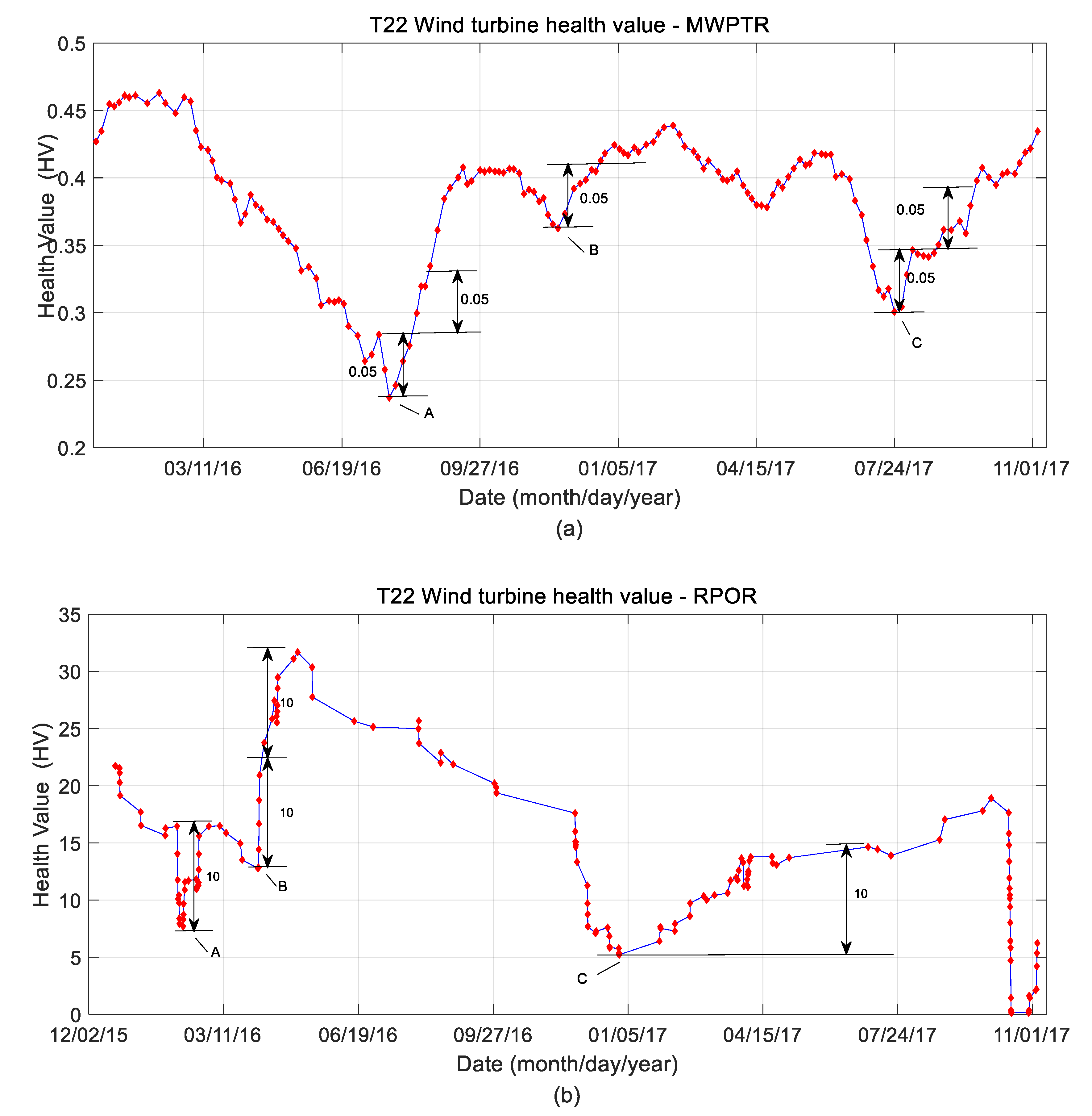
Condition pre-warnings are especially important for the operation and maintenance staff of in a wind farm. Using the PAM method, the T22 HV curves for the MWPTR and RPOR from 20 May 2015 to December 2017 were calculated. The HV in the MWPTR corresponds to the deviation of the actual measured data and the baseline data. Presuming a deviation of 0.05 is set as the alarm threshold, a point larger than the minimum points by 0.05 is selected as the pre-warning point. The HV curve and pre-warning line are plotted, as shown in Figure 15a, in which the minimum power point of the HV curve are marked as A, B and C. The growth rate of the HV curve after Date A is larger than 0.1. The HV of Date B is much larger than that for Date A, and the growth rate of the HV curve after date B exceeds 0.05. The HV of Date C is less than that of Date B but larger than that of Date A, of which the later growth rate exceeds 0.1. This analysis indicates that the HV curve of T22 changes considerably; in other words, the wind turbine performances are unstable. If the degradation trend after the minimum point is detected by the threshold line with HV equal to 0.05 and effective maintenance activities are carried out, a worsening in the degradation trend can be avoided. Similarly, when the minimum power point exceeds 0.1, the maintenance staff should focus extensively on investigating the reason.
In the wind farm considered in the research, the generator power limit is 2067.6 kW, the mean power of the baseline data is approximately 2013 kW, and their difference is 54.6 kW, which is the theoretical deviation value in the RPOR area. The threshold is set as 10 kW in the RPOR, the minimum power of the HV curve is selected, and the warning line with HV equal to 10 is plotted, as shown in Figure 15b. It can be seen that after the HV curve of Date A increases gradually with a span larger than 10 kW, it decreases gradually to Date B. The continuous increasing rate after Point B exceeds 20 kW and reaches the global maximum, and the growth rate of the HV curve after Date C exceeds 10 kW. Therefore, using the proposed method to determine the HV curves and setting the threshold value line after the minimum power, an early warning can be triggered when the HV exceeds the threshold value so that further degradation can be avoided through maintenance.

6. Conclusions

This paper proposes a method for evaluating the working wind turbine power performance by calculating variations between the actual wind-power data and the baseline wind-power data from the SCADA system. The HV curve of wind turbine is calculated by the present method. The result from the proposed method on the MWPT region has been validated with the PC2-Dev method. In the RPOR region, the present method is also benchmarked with the traditional statistic mean and variance method. The computed results show the present method can effectively quantify variations between the actual and reference wind-power data. The performance results can effectively reflect the operational status of wind turbines; furthermore, they are able to be understood by engineers, and they provide important information for the operations and maintenance of wind turbines.
The purpose of this work is to propose an effective tool for assessment the power performance of wind turbines. Power generation depends not only on the wind speed but also on the turbine conditions, such as the operating factors, yaw angle, and wind turbulence. To find change causes or detect anomalies, more data need be analyzed. In future work, the authors intend to investigate the reasons for these anomalies and perform fault identification. In addition, the current method only considered wind speed and power. The wind direction, air density and temperature have a considerable impact on the power of wind turbines and should be studied.

Author Contributions

Data curation, X.Y.; project administration, Q.Z.; resources, A.Z.; writing—original draft, Z.X. All authors have read and agreed to the published version of the manuscript.

Funding

This work is supported by National Key Research and Development Program of People’s Republic of China (grant number 2016YFF0203400), National Natural Science Foundation of People’s Republic of China (grant number 51875199 and 51905165), Hunan Provincial Natural Science Foundation (grant number 2019JJ50186) and Scientific Research Fund of Hunan Provincial Education Department (grant number 18C034).

Conflicts of Interest

The authors declare no conflicts of interest.

References

  1. Hameed, Z.; Hong, Y.S.; Cho, Y.M.; Ahn, S.H.; Song, C.K. Condition monitoring and fault detection of wind turbines and related algorithms: A review. Renew. Sustain. Energy Rev. 2009, 13, 1–39. [Google Scholar] [CrossRef]
  2. Stetco, A.; Dinmohammadi, F.; Zhao, X.; Robu, V.; Flynn, D.; Barnes, M.; Keane, J.; Nenadic, G. Machine learning methods for wind turbine condition monitoring: A review. Renew. Energy 2019, 133, 620–635. [Google Scholar] [CrossRef]
  3. Gao, Z.; Sheng, S. Real-time monitoring, prognosis, and resilient control for wind turbine systems. Renew. Energy 2018, 116, 1–4. [Google Scholar] [CrossRef]
  4. Jia, X.; Jin, C.; Buzza, M.; Di, Y.; Siegel, D.; Lee, J. A deviation based assessment methodology for multiple machine health patterns classification and fault detection. Mech. Syst. Signal Process. 2018, 99, 244–261. [Google Scholar] [CrossRef]
  5. Wang, X.; Zhao, Q.C.; Yang, X.B.; Zeng, B. Condition monitoring of wind turbines based on analysis of temperature-related parameters in supervisory control and data acquisition data. Meas. Control 2019. [Google Scholar] [CrossRef] [Green Version]
  6. Staffell, I.; Green, R. How does wind farm performance decline with age? Renew. Energy 2014, 66, 775–786. [Google Scholar] [CrossRef] [Green Version]
  7. Roscher, B.; Werkmeister, A.T.; Schelenz, R.; Jacobs, G. Estimation of 1Hz Distribution based on 10min SCADA Data. In Proceedings of the Offshore Wind R&D Conference 2018, Bremerhaven, Germany, 14–16 November 2018. [Google Scholar]
  8. Li, J.L.; Zhang, X.R.; Zhou, X.; Lu, L.Y. Reliability assessment of wind turbine bearing based on the degradation-Hidden-Markov model. Renew. Energy 2019, 132, 1076–1087. [Google Scholar] [CrossRef]
  9. Gao, Z.; Ding, S.X.; Cecati, C. Real-time fault diagnosis and fault-tolerant control. IEEE Trans. Ind. Electron. 2015, 62, 3752–3756. [Google Scholar] [CrossRef] [Green Version]
  10. Gao, Z.; Cecati, C.; Ding, S.X. A survey of fault diagnosis and fault-tolerant techniques-part II: Fault diagnosis with knowledge-Based and hybrid/active approaches. IEEE Trans. Ind. Electron. 2015, 62, 3768–3774. [Google Scholar] [CrossRef] [Green Version]
  11. IEC, IEC 61400-12-1. Wind Turbines—Part 12-1: Power Performance Measurements of Electricity Producing Wind Turbines; International Electrotechnical Commission: Geneva, Switzerland, 2005. [Google Scholar]
  12. Taslimi-Renani, E.; Modiri-Delshad, M.; Elias, M.F.M.; Rahim, N.A. Development of an enhanced parametric model for wind turbine power curve. Appl. Energy 2016, 177, 544–552. [Google Scholar] [CrossRef]
  13. Zhang, F.; Wen, Z.; Liu, D.; Jiao, J.; Wan, H.; Zeng, B. Calculation and Analysis of Wind Turbine Health Monitoring Indicators Based on the Relationships with SCADA Data. Appl. Sci. 2020, 10, 410. [Google Scholar] [CrossRef] [Green Version]
  14. Lee, J. Measurement of machine performance degradation using a neural network model. Comput. Ind. 1996, 30, 193–209. [Google Scholar] [CrossRef]
  15. Dai, J.C.; Liu, D.S.; Wen, L.; Long, X. Research on power coefficient of wind turbines based on SCADA data. Renew. Energy 2016, 86, 206–215. [Google Scholar] [CrossRef]
  16. Park, J.Y.; Lee, J.K.; Oh, K.Y.; Lee, J.S. Development of a novel power curve monitoring method for wind turbines and its field tests. IEEE Trans. Energy Convers. 2014, 29, 119–128. [Google Scholar] [CrossRef]
  17. Kusiak, A.; Zheng, H.; Song, Z. On-line monitoring of power curves. Renew. Energy 2009, 34, 1487–1493. [Google Scholar] [CrossRef]
  18. Cambron, P.; Lepvrier, R.; Masson, C.; Tahan, A.; Pelletier, F. Power curve monitoring using weighted moving average control charts. Renew. Energy 2016, 94, 126–135. [Google Scholar] [CrossRef]
  19. Long, H.; Wang, L.; Zhang, Z.; Song, Z.; Xu, J. Data-Driven Wind Turbine Power Generation Performance Monitoring. IEEE Trans. Ind. Electron. 2015, 62, 6627–6635. [Google Scholar] [CrossRef]
  20. Guo, P.; Infield, D. Wind Turbine Power Curve Modeling and Monitoring with Gaussian Process and SPRT. IEEE Trans. Sustain. Energy 2018, 11. [Google Scholar] [CrossRef] [Green Version]
  21. Papatheou, E.; Dervilis, N.; Maguire, A.E.; Campos, C.; Antoniadou, I.; Worden, K. Performance monitoring of a wind turbine using extreme function theory. Renew. Energy 2017, 113, 1490–1502. [Google Scholar] [CrossRef]
  22. De la Hermosa, R.R.; González-Carrato, R. Wind farm monitoring using Mahalanobis distance and fuzzy clustering. Renew. Energy 2018, 123, 526–540. [Google Scholar]
  23. Gill, S.; Stephen, B.; Galloway, S. Wind Turbine Condition Assessment through Power Curve Copula Modeling. IEEE Trans. Sustain. Energy 2012, 3, 94–101. [Google Scholar] [CrossRef] [Green Version]
  24. Marvuglia, A.; Messineo, A. Monitoring of wind farms’ power curves using machine learning techniques. Appl. Energy 2012, 98, 574–583. [Google Scholar] [CrossRef]
  25. Lapira, E.; Brisset, D.; Ardakani, H.D.; Siegel, D.; Lee, J. Wind turbine performance assessment using multi-regime modeling approach. Renew. Energy 2012, 45, 86–95. [Google Scholar] [CrossRef]
  26. Skrimpas, G.A.; Sweeney, C.W.; Marhadi, K.S.; Jensen, B.B.; Mijatovic, N.; Holbll, J. Employment of Kernel Methods on Wind Turbine Power Performance Assessment. IEEE Trans. Sustain. Energy 2015, 6, 698–706. [Google Scholar] [CrossRef]
  27. Jia, X.; Jin, C.; Buzza, M.; Wang, W.; Lee, J. Wind turbine performance degradation assessment based on a novel similarity metric for machine performance curves. Renew. Energy 2016, 99, 1191–1201. [Google Scholar] [CrossRef]
  28. Dai, J.C.; Yang, W.X.; Cao, J.W.; Liu, D.S.; Long, X. Ageing assessment of a wind turbine over time by interpreting wind farm SCADA data. Renew. Energy 2018, 116, 116,199–208. [Google Scholar] [CrossRef] [Green Version]
  29. Ester, M.; Kriegel, H.P.; Xu, X. A density-based algorithm for discovering clusters a density-based algorithm for discovering clusters in large spatial databases with noise. In Proceedings of the 2nd International Conference on Knowledge Discovery & Data Mining, Portland, OR, USA, 2–4 August 1996; pp. 226–231. [Google Scholar]
  30. Daszykowski, M.; Walczak, B.; Massart, D.L. Looking for natural patterns in data: Part 1. Density-based approach. Chemom. Intell. Lab. Syst. 2001, 56, 83–92. [Google Scholar] [CrossRef]
  31. Daszykowski, M.; Walczak, B.; Massart, D.L. Looking for natural patterns in analytical data. Part 2. Tracing local density with OPTICS. J. Chem. Inf. Comput. Sci. 2016, 42, 500. [Google Scholar] [CrossRef]
  32. Mahmoud, H.M. Sorting: A Distribution Theory; John Wiley & Sons: Hoboken, NJ, USA, 2000; ISBN 978-04713978-047132710327103. [Google Scholar]
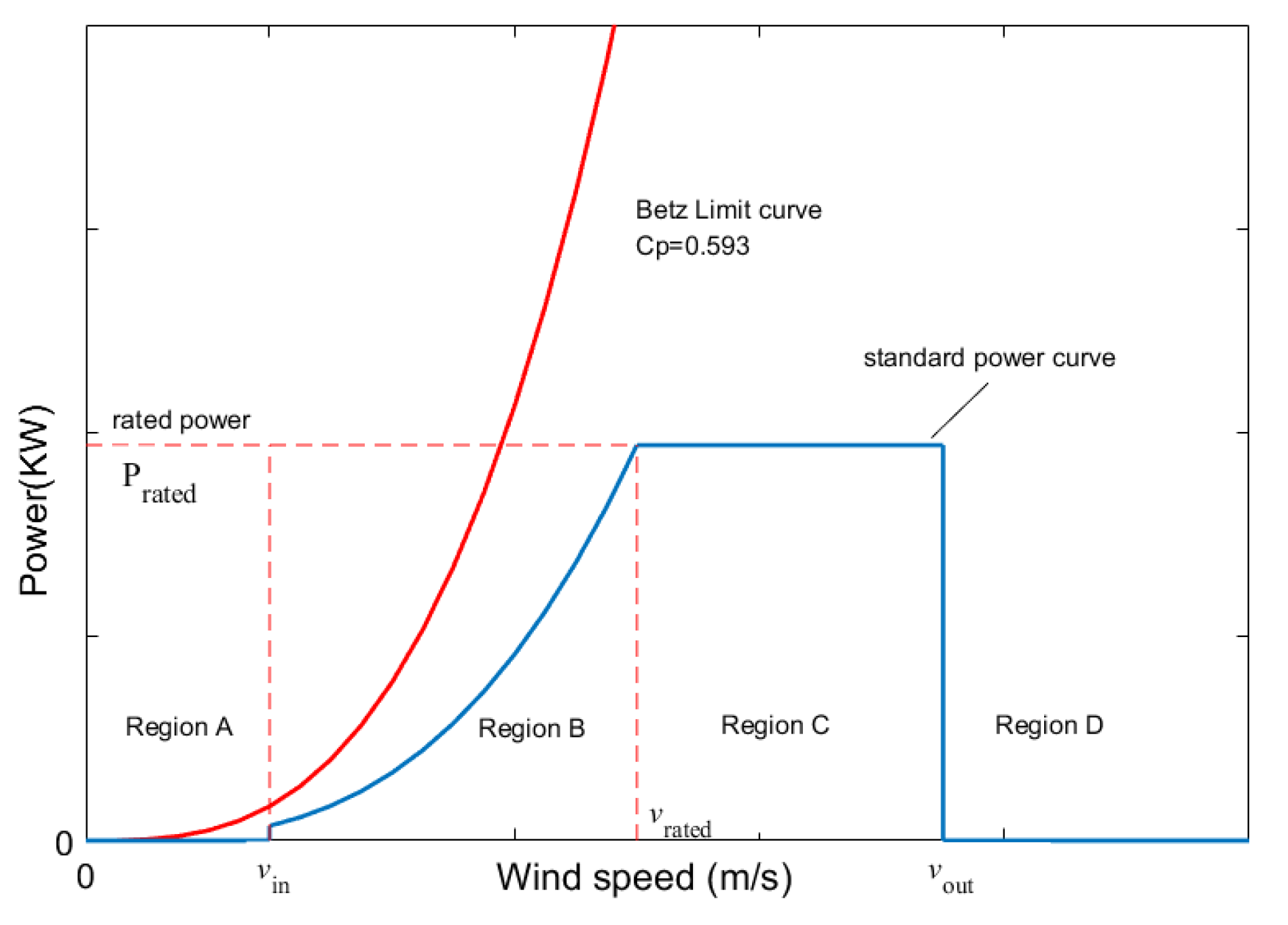
Figure 1. Power curve of a pitch-regulated wind turbine.
Applsci 10 03268 g001
Figure 2. Baseline and actual measurement wind-power data which are cleaned.
Applsci 10 03268 g002
Figure 3. Illustration of probabilistic area metric.
Applsci 10 03268 g003
Figure 4. Process flow of the performance assessment method.
Applsci 10 03268 g004
Figure 5. Method to update time window.
Applsci 10 03268 g005
Figure 6. Health result of T01 obtained using the probabilistic area metric (PAM) method in the maximum wind power tracking region (MWPTR).
Applsci 10 03268 g006
Figure 7. Comparative analysis of Dates A, B and C.
Applsci 10 03268 g007
Figure 8. Health assessment result of T01 wind turbine obtained using two methods.
Applsci 10 03268 g008
Figure 9. Health assessment result of T07 wind turbine obtained using two methods.
Applsci 10 03268 g009
Figure 10. Comparative data analysis of Date A and Date B (a) Baseline data and data of date A and data B; (b) Data of date A and data B; (c)Overlap data of date A and B; (d) Nonoverlap data of date A and B.
Applsci 10 03268 g010aApplsci 10 03268 g010b
Figure 11. Power time series curve of T22 in the rated power output region (RPOR).
Applsci 10 03268 g011
Figure 12. HV curve of T22 wind turbine obtained using the PAM in the RPOR.
Applsci 10 03268 g012
Figure 13. Power time series for different dates (dashed line represents the mean, and the black line indicates the rated power).
Applsci 10 03268 g013
Figure 14. Comparison of two wind turbines.
Applsci 10 03268 g014
Figure 15. Early warning for wind turbines based on health value curve (a) Health value curves of T22 wind turbine in the MWPTR with the PAM method; (b) Health value curves of T22 wind turbine in the PROR with the PAM method.
Applsci 10 03268 g015
Table 1. State parameters for different dates.
DateHealth ValueMean Value (KM)Standard Deviation (std)
Baseline Data020133.6
Point F5.21201510.65
Point B7.071201213.97
Point G18.92199415.75
Point A21.74199219.39
Point E31.66198116.84