According to
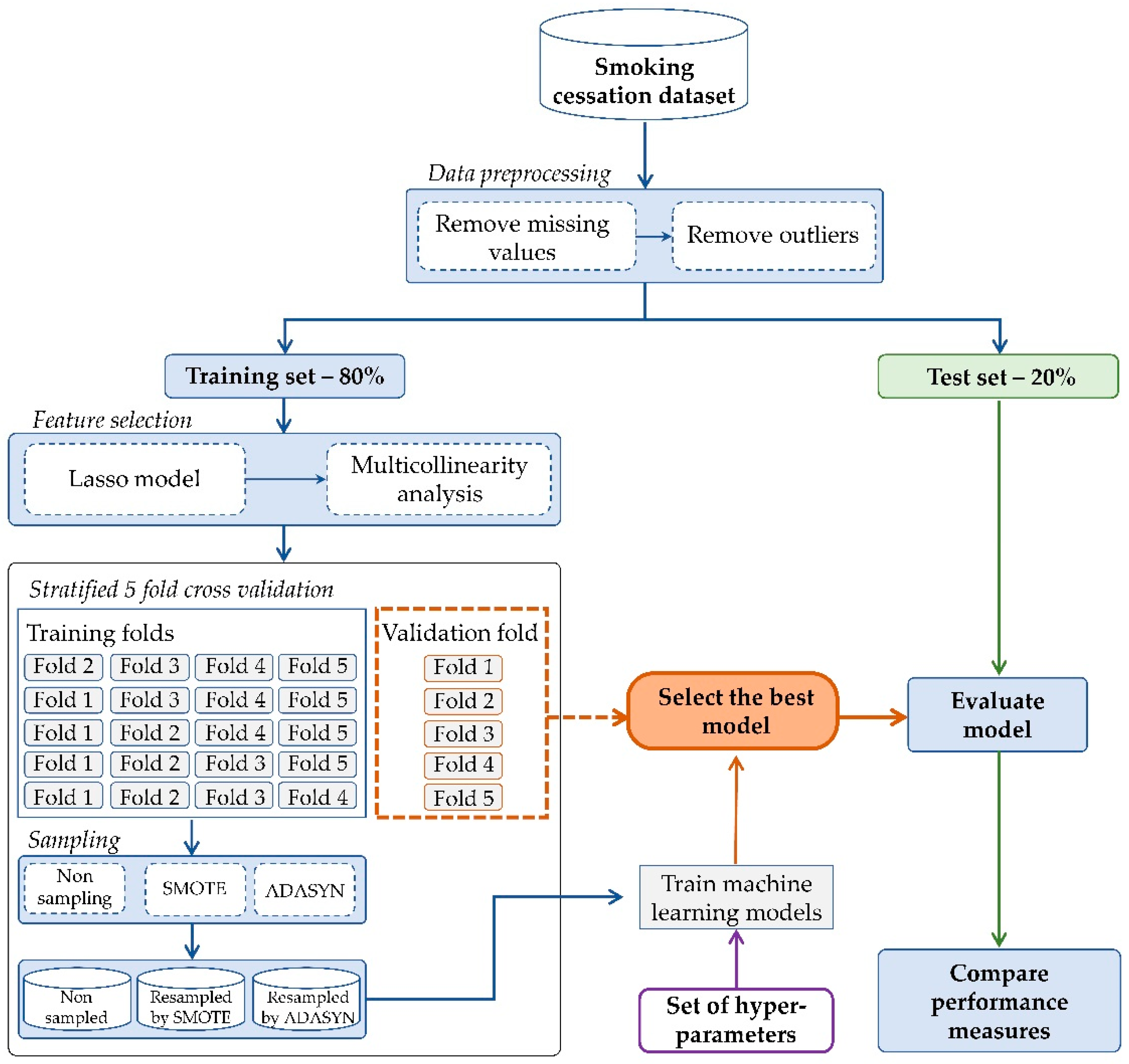
Figure 1, the proposed experimental design requires the execution of the number of components: (I) feature selection, (II) oversampling following by (III) comparison between synthetic oversampling techniques and machine learning classifiers for prediction models of the smoking cessation intervention. Moreover, non-parametric Friedman’s test is applied to ensure the differences between the results of the prediction models are significant. In addition, the best representative features were provided, which were used to build the best ranked predictive models.
4.1. Subjects and Dataset
The experimental dataset is taken from the Korea National Health and Nutrition Examination Survey (KNHANES), which is conducted by the Korea Centers for Disease Control and Prevention (KCDC). The KNHANES dataset contains a health examination for various numbers of diseases, health interview, and nutrition surveys. In this way, some considerable necessary features were surveyed from a minor of the population with around only one year. Therefore, the dataset contains features that have a large number of missing values and outliers. We have analyzed the dataset collected from 2009 to 2017 among the Korean population, after acquiring permission from the KCDC (
http://knhanes.cdc.go.kr).
Regarding the classification target, it needs to generate the target population for eliminating irrelevant features and instances. Additionally, only adults aged 18 years or older who were considered for smoking-related surveys. Current and former smokers were defined as those who have smoked at least 100 cigarettes in their life. On the contrary, individuals who have never smoked or have smoked less than 100 cigarettes in their life were considered as non-smokers. Initially, the total number of subjects was 75,292, constituting the total number of the collected data. Similar to the literature [
22,
23,
31], we selected 22 features. Subjects were eliminated from the current study based on the following exclusion criteria:
We excluded 53,850 subjects who never smoked.
We excluded 9271 subjects who never tried to quit smoking cigarettes in their life by smoking cessation methods.
The smoking cessation methods of the KNHANES dataset consist of interventions such as smoking quit agent, smoking quit clinic of the public health center, doctor prescribed medication, and no smoking guides by telephone, internet and various kind of counseling, which were used to determine class labels. Then, 8479 subjects were excluded due to missing value and outliers, which were stored in given initial features. The outliers and extreme values were removed based on the interquartile range. The exclusion process of missing value and outlier produced the 3692 subjects with 22 features. According to the classification target, we use the “smoking status of adult” feature that has three groups such as smoking”, “sometimes smoking” and “quit smoking”. In this study, “smoking” and “sometimes smoking” are considered as unsuccessful smoking quitters, whereas “quit smoking” is defined as a successful quitter, which means a person who used to smoke but had not smoked in the past 1 year.
Descriptive characteristics of the former and current smokers are provided in
Table 2. Consequently, 951 (25.7%) of the smokers can quit smoking habit successfully after attending at least one smoking cessation intervention voluntarily. This target class is recognized by imbalanced distribution. In comparison to socio-demographic features, we found evidence that approximately 90% of subjects were men among former and current smokers. Men were more likely to smoke than women; thus, 856 (25.9%) of men and 95 (24.4%) of women were resulted by successfully smoking quitters in our study. For the age group, (<35 years) subjects were less likely to quit smoking than other age groups. Taken together, 14.09% of <35 years, 21.90% of 36–45 years, 26.30% of 46–55 years and 40.89% of >56 years had successfully quit smoking. Among the body mass index, lower weights (13.0–19.0) of subjects were markedly less likely to quit smoking by about 7% than other groups. Among the smoking cessation rates by the urban and rural population, urban areas had two times higher successful quit rates than rural. Therefore, the subjects starting smoking in age groups 27.01% of <18 years, 23.40% of 19–24 years and 28.05% of >25 years were estimated to quit smoking, respectively. Thus, subjects who started to smoke in the age group of 19–24 years are less likely to quit smoking than other age groups.
4.2. Feature Selection
The feature selection component consists of two phases, such as the lasso method and multicollinearity analysis. It is well known that the lasso method helps to increase the prediction of the model by removing irrelevant features that are not related to target classes. The lasso feature selection method is identified irrelevant features as “Residence area”, “Employment condition”, “Average sleep time per day”, “Stress level” and “Long term depression (more than two weeks)” that eliminated by assigning them a coefficient equal to zero. On the contrary, the remaining 17 of the 22 features estimated along with non-zero coefficients, which were selected by sufficiently representative features.
We directly verify to check the collinearity between selected features using multicollinearity in regression analysis after eliminating the non-significant features, which are passed in the lasso method.
Figure 2 illustrates the result of the Variance Inflation Factor (VIF) value for all independent features. Generally, it is suspected that multicollinearity will present if the VIF lies between 5 and 10. If the VIF value is greater than those values, it investigates a high correlation among features that remains problematic. As can be seen, none of the features have detected the presence of multicollinearity issue in the multiple linear regression models. In total, 17 features and 3682 subjects remained in the end of this component and are is used as inputs to the next components.
4.4. Results and Comparison
In this section, we summarize the overall comparison results that were attained over various machine learning methods.
Table 3 shows the results of the classifiers on imbalanced and balanced data among all subjects and highest performance of evaluation metrics are marked in bold.
As shown in
Table 3, the KNN classifier performed the worst type II error of 0.2490 and F-score of 0.7604. On the contrary, the MLP classifier obtained the best type II error of 0.0500 and SVM achieved the highest F-score of 0.8343. As can be seen, it is hard to build the prediction model with a high geometric mean in terms of the highest type I error in imbalanced data; moreover, this error indicates that successful smoking quitters are misclassified as failed during the intervention. Dealing with the type I error issue under the class imbalance problem, we have applied the SMOTE and ADASYN oversampling techniques. The comparison result shows that the SMOTE with GBT classifier achieved the highest F-score of 0.8888, a balanced accuracy of 0.7928, a geometric mean of 0.7868 and a low type I error of 0.3044 when the learning rate was 0.005 and the number of the tree was 750. The lowest type II errors of 0.0405 and 0.0440 were achieved by the SMOTE with deep MLP, MLP classifiers, respectively. With regard to the evaluation metrics, SMOTE with GBT, MLP classifiers reached the highest results in all subjects.
In this study, our experimental dataset includes 3303 (89.46%) men and 389 (10.54%) women, whereas the former smokers’ target includes 856 (23.20%) men and 95 (2.60%) women, and the current smokers’ target includes 2447 (66.30%) men and 294 (8.00%) women. It is clearly shown that men have a tendency to use tobacco at higher rates than women; moreover, it is important to construct the prediction models for each gender. The evaluation results of prediction models among men and women are summarized in
Table 4 and
Table 5.
For the data sample of men, the best model was distinguished by SMOTE with an RF classifier in terms of the f-score, type II error, balanced accuracy and geometric mean, which reached 0.8952, 0.1364, 0.8116 and 0.8099 when the number of trees is 250 and the criterion is entropy parameters. The SVM classifier performed the better type I error of 0.0365, but it performed the lowest geometric mean of 0.3625 due to worst type II error of 0.8636. Following this, the second best performances were yielded by the ADASYN with the RF classifier when the parameters for the number of trees was 250 and the criterion is gini, as shown in
Table 4.
As seen in
Table 5, the prediction models of women were hardly affected by the imbalanced distribution because the highest type I errors were reached by the baseline classifiers. In terms of type I errors, classifiers performed the lowest balanced accuracy and geometric mean metrics. However, ADASYN with MLP classifier exhibited better balanced accuracy of 0.7735, the geometric mean of 0.7603 and lowest type I error of 0.3684, significantly. In addition, the best f-score of 0.9134 was achieved by the ADASYN with LR.
Comparing to the evaluation performances are shown in
Table 3,
Table 4 and
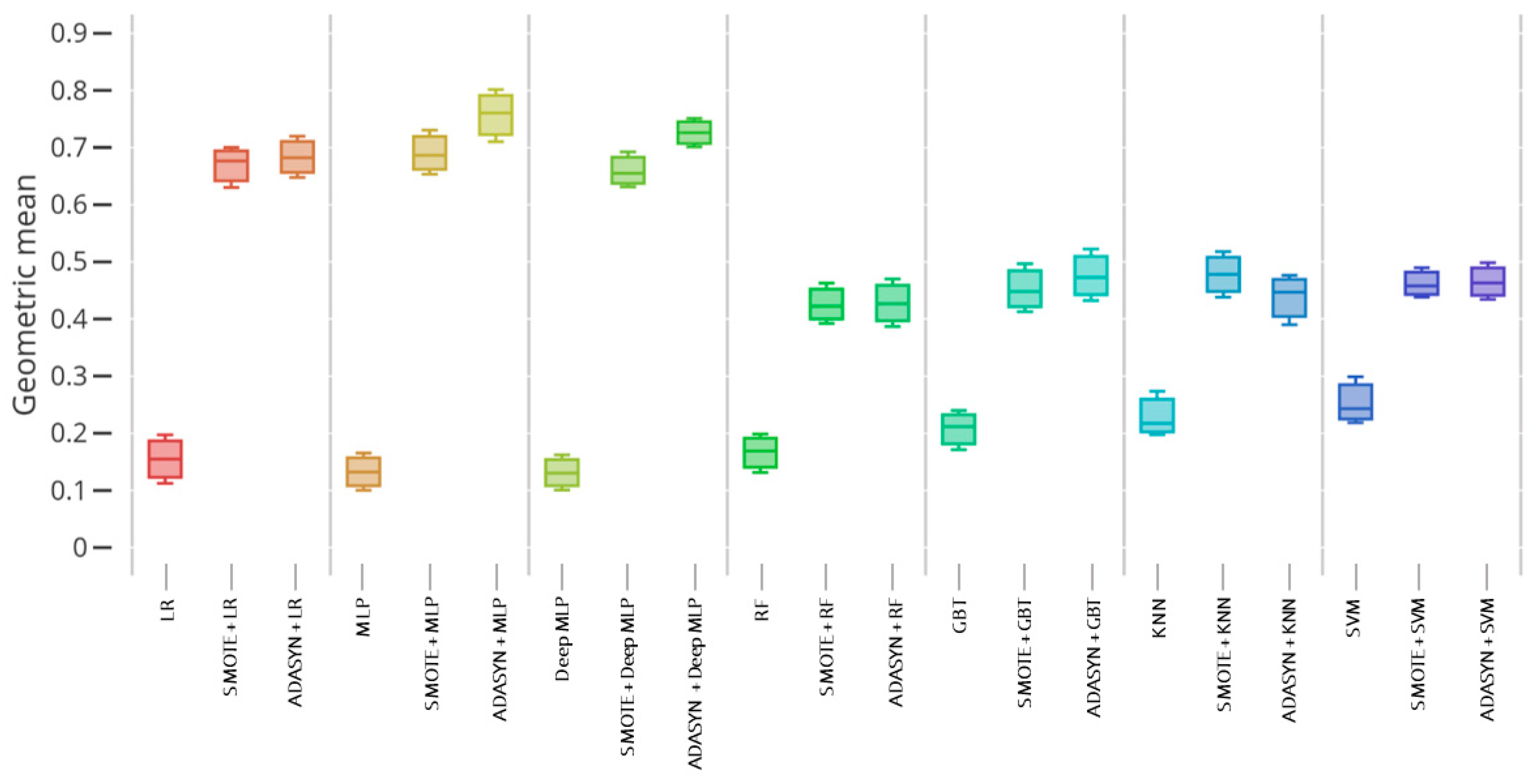
Table 5, certainly type I error issue is the biggest challenge in imbalanced data when it occurs our minority class for successful smoking quitters are misclassified as failed after smoking cessation intervention. Correspondingly, type II error occurs when current smokers are misclassified as successful quitters. Our comparison results revealed significant improvements in prediction models among all subjects and each gender when utilizing the SMOTE and ADASYN oversampling techniques. It is shown that geometric mean suits are one of the proper metrics for ascertaining between critical type I and type II errors. Therefore, concerning the geometric mean,
Figure 3,
Figure 4 and
Figure 5 illustrate the boxplot of the prediction models among all subjects, men and women.
As depicted in
Figure 3, the GBT classifier presented the worst score in non-sampling data, but the SMOTE and ADASYN-based GBT classifier displayed significantly better results among all samples. For the data sample of men, RF and GBT ensemble models reached the best performance when it served the synthetic oversampling techniques, as illustrated in
Figure 4. By way of contrast, the worst performances were performed by KNN and SVM single classifiers among men. Furthermore, ADASYN with the MLP classifier obtained the best prediction model, followed by ADASYN with deep MLP and LR classifiers presented the high scores in a data sample of women, as shown in
Figure 5. Similar to the other samples, single LR, MLP, deep MLP and RF classifiers illustrated the lowest performance due to severe imbalance ratio and small sample data of women. To summarize, single models were inferior to the synthetic oversampling-based models over each sample.
4.4.1. Statistical Test
A non-parametric Friedman test was applied to verify the statistical significance of the differences between the performance results of the various machine learning classifiers. In this study, the prediction models were compared in terms of balanced accuracy score. The Friedman statistic test was calculated as 47.59 with a p-value of and rejected the null hypothesis at a 99% significance level. According to the average ranks of the performances, SMOTE with GBT of 2.33 and SMOTE with RF of 3.33 models performed the top rank compared with other models. GBT, LR and DEEP MLP baseline models were determined low ranks by 20.41, 18.91 and 17.08, respectively.
4.4.2. Model Interpretability
Model interpretability is an important task to get a better understanding of the reasoning behind the prediction models. As a comparison result, GBT and RF classifiers determined the best predictive models when combining with the SMOTE among all subjects. Thus, the most important features for SMOTE with GBT and RF models were provided as shown in
Figure 6 and
Figure 7.
To ensure model interpretability, features were sorted in descending order of their importance scores in model construction. According to the SMOTE with the GBT model, “daily smokers at home”, “age of smoking initiation”, and “attendance in smoking cessation education” were maintained as the most useful features, with scores of 0.089, 0.088 and 0.079, respectively, to predict the smoking cessation target. On the contrary, “attendance in smoking cessation education”, “daily smokers at home” and “household income” features were highly important for constructing the SMOTE with RF model. The highly scored features enhance the rationale decisions in smoking-related health concerns and should be collected in smoking cessation data. Both of the predictive models were constructed by the same features, such as “diabetes” and “hypertension”, with low importance scores. Therefore, this analysis is expected to improve the efficiency and effectiveness of healthcare decision support system in real-world adoption.


