In
Section 4.2.1, for each dataset, we find the
best iterations on which similarity measures show their
highest accuracies. In
Section 4.2.2, for each dataset, we find the
best values of
d (i.e., number of dimensions) for which the embedding methods show their
highest accuracies in similarity computation of nodes. In
Section 4.2.3 and
Section 4.2.5, we present an experimental analysis on the effectiveness and efficiency of embedding methods (i.e., based on their best values of
d) in comparison with similarity measures (i.e., based on their best iterations), respectively.
Section 4.2.4 analyzes the impact of the value of
d on the accuracy of embedding methods.
4.2.2. Graph Embedding Methods: Best Values of d
Now, we apply ATP, BoostNE, DeepWalk, DWNS, graphGAN, Line, NERD, NetMF, and node2vec to our five datasets to obtain the low-dimensional representation vectors of the nodes. Then, to compute the similarity between two nodes in a dataset, we apply Cosine to their corresponding vectors. In order to
carefully analyze the impact of the number of dimensions
d in similarity computation of nodes, we set
d to different values as 64, 128, 256, and 512. For
each possible combination of methods, datasets, and
d values (e.g., ATP with the BlogCatalog dataset when
), we perform the experiment
five times and select the
best accuracy obtained among these five different executions as the
final accuracy for that combination. More specifically, we conducted 900 (
) different experiments. Finally, similar to the strategy taken in
Section 4.2.1, in the case of each embedding method with a dataset, we find out the
best value of
d for which the embedding method shows its
highest accuracy in similarity computation of nodes.
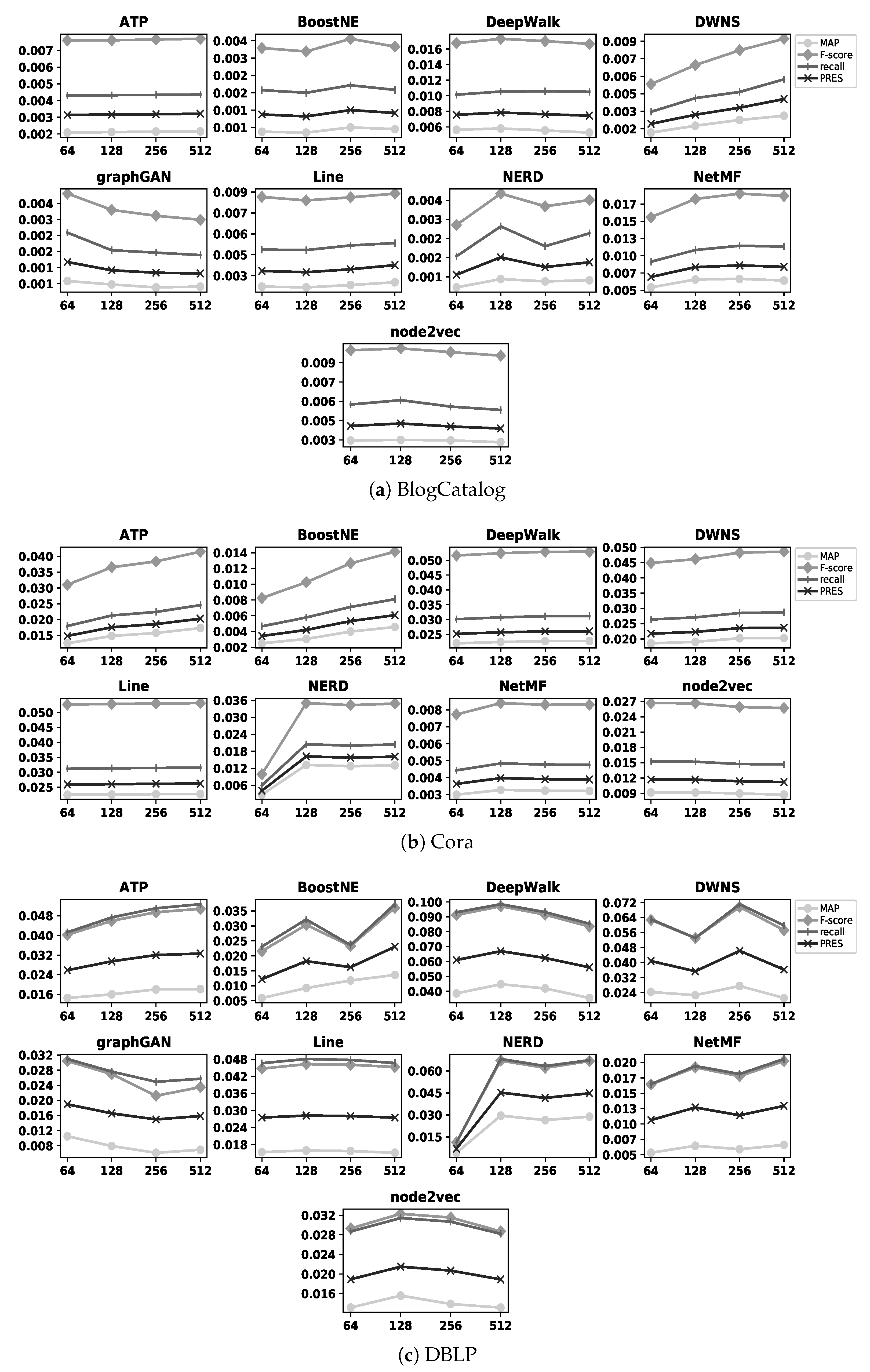
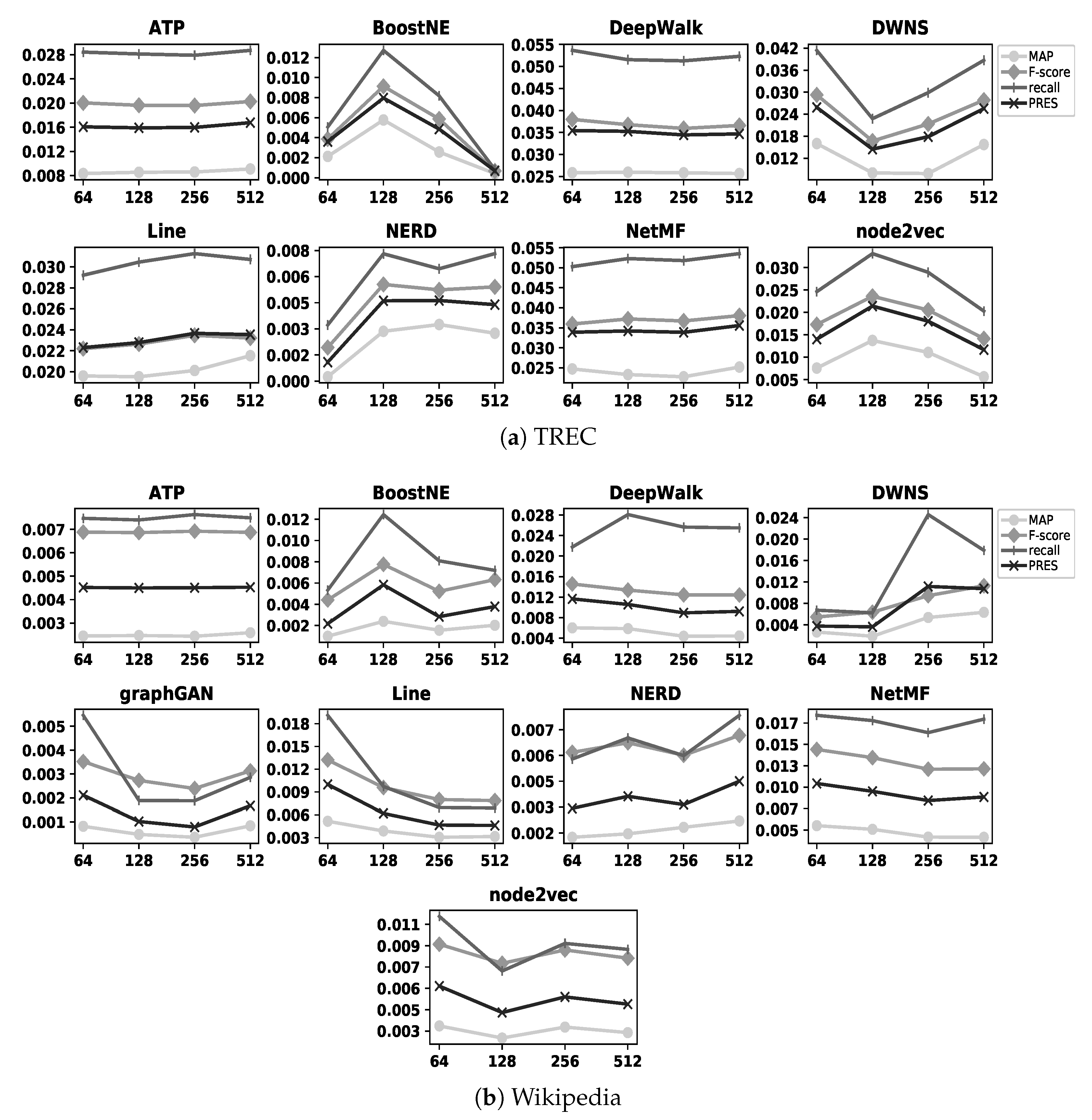
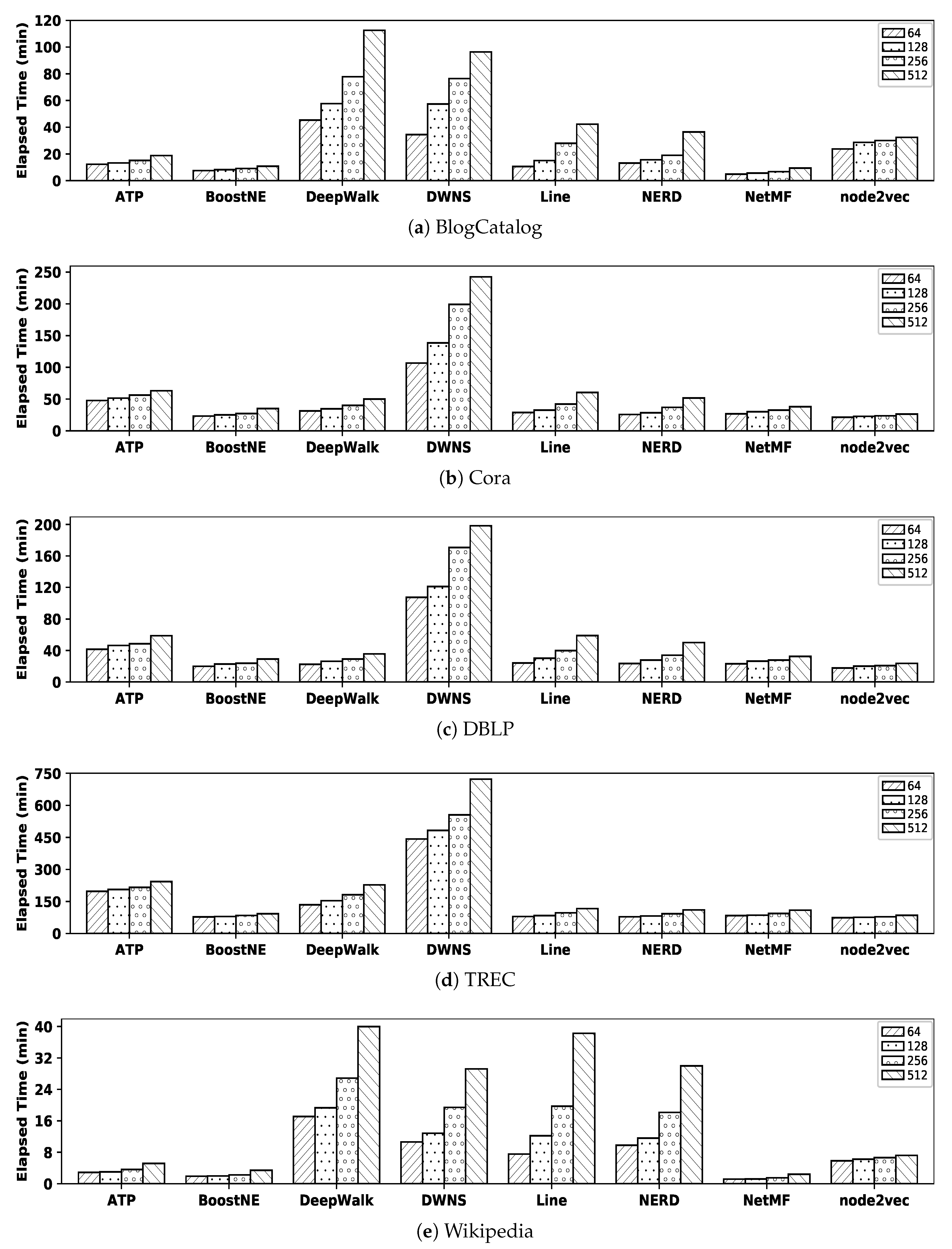
Figure 4 and
Figure 5 illustrate the accuracy of embedding methods with different values of
d. The former figure shows the results with the BlogCatalog, Cora, and DBLP datasets, while the latter one shows the results with the TREC and Wikipedia datasets; as an example, BoostNE shows its highest accuracy when
d is set as 256 and 128 with the BlogCatalog and TREC datasets, respectively. In these figures, we do not represent the precision metric due to the same reason as in
Figure 3; the values of this metric with BlogCatalog, Cora, DBLP, TREC, and Wikipedia datasets for different values of
d are represented in
Table A1,
Table A2,
Table A3,
Table A4 and
Table A5 in
Appendix A, respectively. As already noted in
Section 4.1, we cannot apply graphGAN to the Cora and TREC datasets due to their large sizes.
Table 3 summarizes the best value of
d for all embedding methods with our datasets. Note that, hereafter, when we compare the effectiveness of embedding methods with those of similarity measures for a dataset, we consider the effectiveness of embedding methods
on their best values of d with that dataset; as an example, in the case of DeepWalk with the BlogCatalog dataset, we consider its effectiveness based on
according to
Table 3.
4.2.3. Effectiveness Evaluation
In this section, we analyze the effectiveness (i.e., accuracy) of embedding methods in computing the similarity of nodes and compare it with those of similarity measures with each dataset as follows. As explained in
Section 4.2.1 and
Section 4.2.2, to compare the effectiveness of similarity measures with embedding methods for each dataset in this section,
we consider their accuracies on their best iterations and best values of d represented in
Table 2 and
Table 3, receptively.
Figure 6 illustrates the accuracy of all embedding methods and similarity measures with the BlogCatalog dataset. In this figure, we do not represent the precision measure due to the same reason as in
Figure 3; instead, we show the precision values for all methods in
Table 4. In addition, for those embedding methods and similarity measures that show comparable accuracies, we write down the values of their corresponding MAP, PRES, recall, and F-score in the figure to have better comparison.
As observed in the figure, with the BlogCatalog dataset, NetMF shows the
highest accuracy among all the embedding methods in terms of MAP, precision, recall, PRES, and F-score; however, its accuracy is
close to that of DeepWalk, while BoostNE, graphGAN, and NERD show the
worst accuracies. SimRank* shows
better accuracy than other similarity measures, while SimRank shows the
worst accuracy in terms of MAP, precision, recall, PRES, and F-score. Now, by comparing the accuracy of NetMF with that of SimRank*, it is observed that NetMF
outperforms SimRank* by 73.44%, 35.68%, 42.89%, 50.00%, and 47.10% in terms of MAP, precision, recall, PRES, and F-score, respectively;
Table 5 shows the
percentage of improvements in accuracy obtained by NetMF over all other methods with the BlogCatalog dataset.
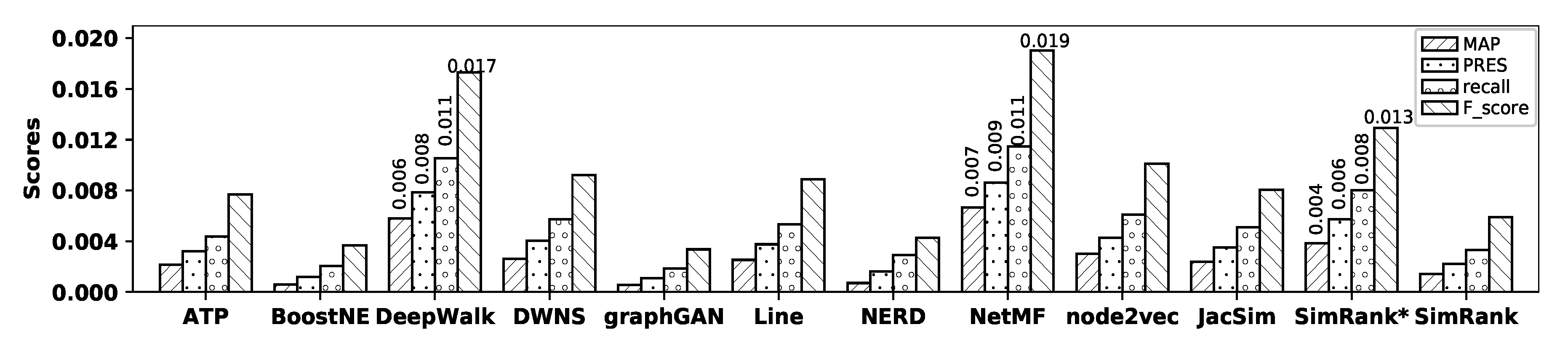
Figure 7 illustrates the accuracy of all embedding methods and similarity measures with the Cora dataset and
Table 6 shows the precision values for all methods.
As observed in the figure, with the Cora dataset, although DeepWalk and Line show the
best accuracy among all embedding methods, their accuracies are
not tangible; Line outperforms DeepWalk in terms of recall, PRES, and F-score, while DeepWalk outperforms Line in terms of MAP and precision. NetMF and BoostNE show the worst accuracy among embedding methods in terms of all metrics. In the case of similarity measures, JPRank shows the
best accuracy and SimRank again shows the worst one in terms of MAP, precision, recall, PRES, and F-score. Now, by comparing the accuracy of Line with that of JPRank, it is observed that JPRank slightly
outperforms Line by 4.05%, 5.73%, 2.28%, 2.98%, and 3.05% in terms of MAP, precision, recall, PRES, and F-score, respectively;
Table 7 shows the percentage of improvements in accuracy obtained by JPRank over all other methods with the Cora dataset.
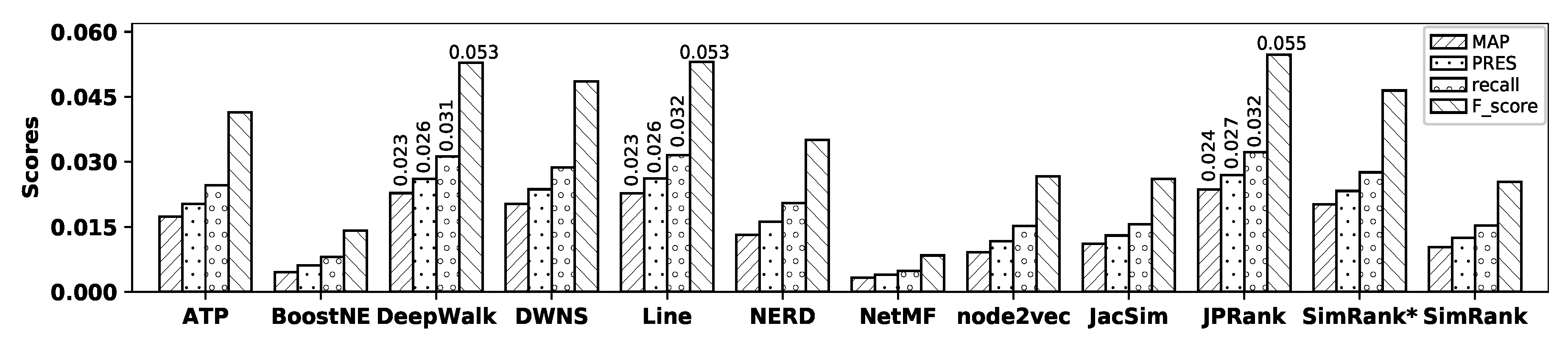
Figure 8 illustrates the accuracy of all embedding methods and similarity measures with the DBLP dataset and
Table 8 shows the precision values for all methods.
As observed in the figure, DeepWalk shows the
best accuracy among all embedding methods, while NetMF shows the worst one in terms of MAP, precision, recall, PRES, and F-score. Among similarity measures, JPRank shows the
best accuracy and it is
close to that of JacSim, while SimRank shows the worst accuracy in terms of all metrics. Now, by comparing the accuracy of DeepWalk with that of JPRank, it is observed that JPRank
outperforms DeepWalk by 64.89%, 50.34%, 51.70%, 52.71%, and 51.11% in terms of MAP, precision, recall, PRES, and F-score, respectively;
Table 9 shows the percentage of improvements in accuracy obtained by JPRank over all other methods with the DBLP dataset.
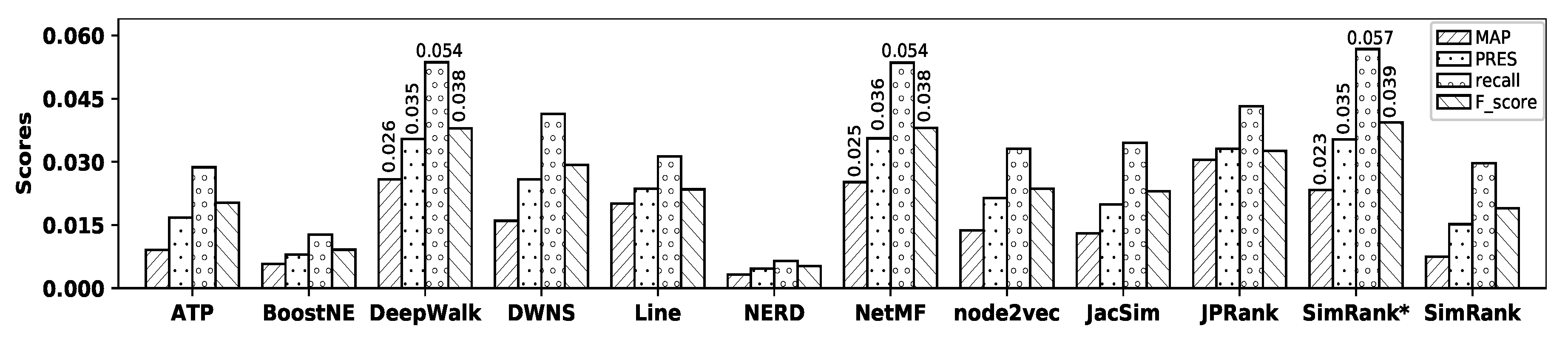
Figure 9 illustrates the accuracy of all embedding methods and similarity measures with the TREC dataset and
Table 10 shows the precision values for all methods.
As observed in the figure, DeepWalk and NetMF show the best accuracy among all embedding methods in terms of MAP, precision, recall, PRES, and F-score. However, their accuracies are
not tangible, where NetMF outperforms DeepWalk in terms of precision, PRES, and F-score, while DeepWalk shows better accuracy in terms of MAP and recall. NERD shows the worst accuracy among all embedding methods. SimRank* shows the
best accuracy among all similarity measures, while SimRank shows the worst one in terms of all metrics. Now, by comparing the accuracy of NetMF with that of SimRank*, it is observed that they show very
close accuracy; SimRank* outperforms NetMF in terms of precision, recall, and F-score, while NetMF outperforms SimRank* in terms of MAP and PRES.
Table 11 shows the percentage of improvements in accuracy obtained by SimRank* over all other methods with the TREC dataset.
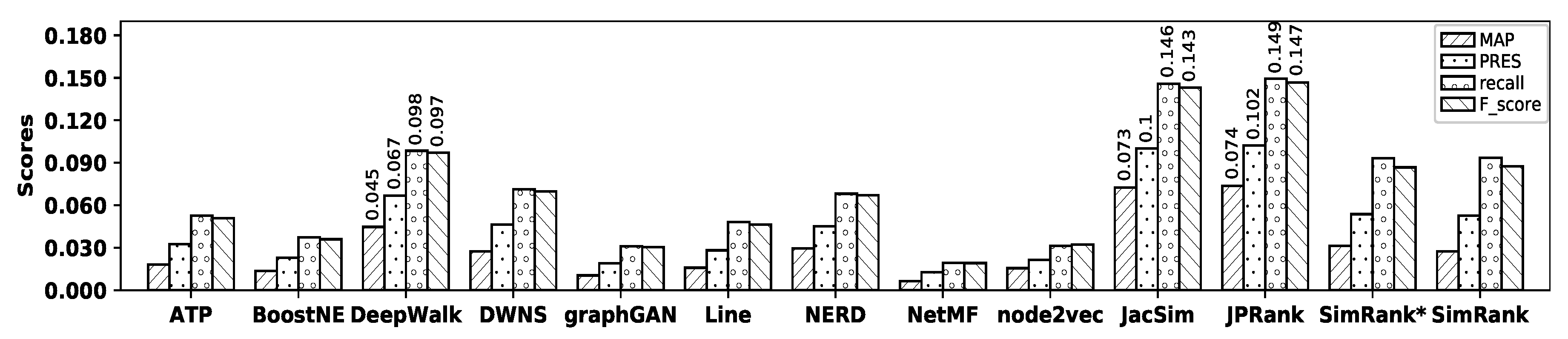
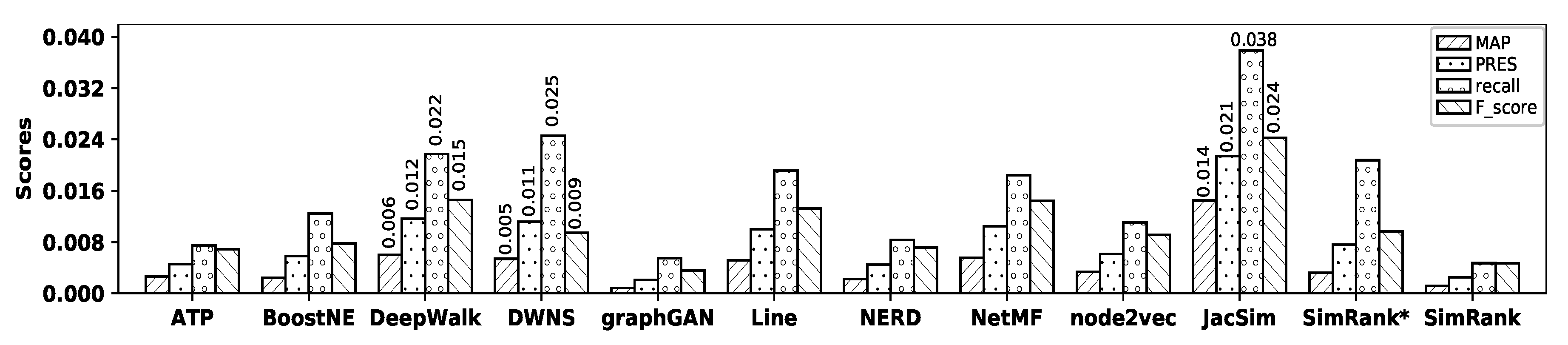
Figure 10 illustrates the accuracy of all embedding methods and similarity measures with the Wikipedia dataset, and
Table 12 shows the precision values for all methods. As observed in the figure, DeepWalk shows the
highest accuracy among embedding methods in terms of MAP, precision, recall, PRES, and F-score; however, its accuracy is close to that of DWNS, while graphGAN shows the
worst accuracy. Among similarity measures, JacSim shows the best accuracy, while SimRank shows the worst one in terms of all metrics. Now, by comparing the accuracy of DeepWalk with that of JacSim, it is observed that JacSim
outperforms DeepWalk by 140.20%, 34.91%, 74.16%, 83.45%, and 66.55% in terms of MAP, precision, recall, PRES, and F-score;
Table 13 shows the percentage of improvements in accuracy obtained by JacSim over all other methods with the Wikipedia dataset.
4.2.4. Impact of d on Accuracy of Embedding Methods
In this section, we analyze whether
increasing the number of dimensions
improves the effectiveness of embedding methods in computing the similarity of nodes. In
Section 4.2.2,
Figure 4 illustrates the accuracy of all embedding methods with the BlogCatalog, Cora, and DBLP datasets for different values of
d; in addition,
Figure 5 illustrates the results of the same experiments with the TREC and Wikipedia datasets. As observed in these figures, in some cases such as DWNS and NetMF with the BlogCatalog dataset, increasing the number of dimensions
improves the accuracy of the embedding methods (i.e., refer to
Figure 4); on the contrary, in some cases such as Line with the Wikipedia dataset (i.e., refer to
Figure 5) and graphGAN with the BlogCatalog dataset (i.e., refer to
Figure 4), increasing the number of dimensions
adversely affects the accuracy of the embedding methods. In addition, in some cases such as DeepWalk with the DBLP dataset (i.e., refer to
Figure 4) and node2vec with the TREC dataset (i.e., refer to
Figure 5), we observe
both improvement and reduction in accuracy by increasing the number of dimensions. In summary, increasing the value of
d does
not help improve the accuracy of embedding methods in computing the similarity of nodes. In
Section 4.2.2,
Table 3 indicates the value of
d showing the best accuracy for each embedding method with our datasets.
As represented in
Table 3, some embedding methods show their best accuracies when
or
; we call such a case a
suspicious one since it
may possible to improve the accuracy of the embedding method by assigning a lower (i.e., 32) or higher (i.e., 1024) value to
d, respectively. However, if the accuracy of a suspicious case is
not comparable with the accuracy of the
best method in the dataset, conducting the aforementioned experiment is
not beneficial since our overall observations will not be affected by the new result; for example, although ATP with the BlogCatalog dataset shows its highest accuracy when
as a suspicious case, its accuracy is
quite lower than that of NetMF as the best method for the same dataset (refer to
Figure 6). In
Table 3, there are
only four following real suspicious cases that we need to consider them: both DeepWalk and Line show their highest accuracies when
with the Cora dataset and their accuracies are very close to that of JPRank as the best method with Cora (i.e., refer to
Figure 7). In addition, DeepWalk and NetMF show their highest accuracies when
and
with the TREC dataset, respectively; their accuracies are very close to that of SimRank* as the best method with TREC (i.e., refer to
Figure 9). Therefore, we conduct the following four new experiments:
DeepWalk with the Cora dataset and
Line with the Cora dataset and
DeepWalk with the TREC dataset and
NetMF with the TREC dataset and
Table 14 represents the accuracies of the four new experiments (i.e., in bold face) along with the accuracies of their corresponding suspicious cases. In case 1, DeepWalk shows the same accuracy as it does when
; in addition, in cases 2 and 4, Line and NetMF show similar accuracies as they do when
, respectively. In case 3, DeepWalk shows lower accuracy in comparison with
. Therefore, we do
not need to apply any changes in our results represented in
Table 3.
4.2.5. Efficiency Evaluation
In this section, we carefully analyze the efficiency (i.e., execution time) of embedding methods in computing the similarity of nodes and compare it with that of similarity measures.
In order to conduct a fair comparison, we implemented the matrix form of JacSim, JPRank, SimRank*, and SimRank
without applying any acceleration techniques such as multi-processing (as the simplest technique), fine-grained memorization [
9], partial sums memoization [
49], and backward local push and Monte Carlo sampling [
50]. Since the execution time could slightly change depending on the system resources such as CPU overload, to obtain an accurate execution time, we run each similarity measure on eight iterations for five times with a dataset and the average run time over the five executions is regarded as the
final execution time of the similarity measure. Note that we consider
only the elapsed time to compute the similarity scores as the execution time; the required time to store the results of similarity computation in a file or a database is
not considered.
Table 15 shows the execution time (minutes) of similarity measures with our five datasets (As already explained in
Section 4.2.1, we do not apply JPRank to undirected graphs BlogCatalog and Wikipedia). With all datasets, SimRank* shows the best efficiency since it requires only
one matrix multiplication in Equation (A8). With undirected datasets (i.e., BlogCatalog and Wikipedia), JacSim shows the worst efficiency since it requires two matrix multiplications and a pairwise normalization paradigm to compute matrix
E in Equation (A6). With directed datasets (i.e., Cora, DBLP, and TREC), JPRank shows the worst efficiency since it requires four matrix multiplications and two pairwise normalization paradigms to compute matrices
E and
in Equation (A10). However, among
all the available cases in
Table 15, JacSim with the BlogCatalog dataset shows the worst efficiency, although BlogCatalog has less nodes than Cora, DBLP, and TREC datasets. The reason is that there are “32,787,165” node-pairs with non-empty common in-link sets in this dataset, which makes the calculation of matrix
E expensive; the number of these node-pairs in Cora, DBLP, TREC, and Wikipedia datasets are “229,306”, “466,990”, “1,391,293”, and “11,015,803”, respectively.
For embedding methods, the execution time is regarded as the summation of a learning time (i.e., elapsed time to construct low-dimensional representation vectors) and a similarity computation time (i.e., elapsed time to compute the similarity scores of all pairs of representation vectors by employing Cosine). With each dataset, the learning time of an embedding method is regarded as the average run time over the five executions of the method. We implemented Cosine based on a matrix/vector multiplication technique, which is significantly (i.e., almost 30 times) faster than its conventional implementation. In the case of similarity computation time, we consider only the elapsed time to compute the similarity scores by applying Cosine; the required time to store the results in a file or a database is not considered as we did for similarity measures.
Table 16 represents the learning time (minutes) of all embedding methods for different values of
d with all datasets where
bold face numbers indicate the best efficiency with each value of
d in a dataset. As observed in the table, NetMF shows the
best efficiency among
all embedding methods with the BlogCatalog and Wikipedia datasets
regardless of the value of
d, node2vec shows the
best efficiency among all methods with Cora, DBLP, and TREC datasets
regardless of the value of
d, BoostNE, and ATP almost have better efficiency after NetMF and node2vec with all datasets, and graphGAN shows the
worst efficiency among all embedding methods with all datasets regardless of the value of
d.
Table 17 shows the similarity computation time (minutes) based on different vector sizes (i.e.,
) with our five datasets. Note that the similarity computation time for a dataset depends on the
number of node-pairs and the representation vector’s
size (i.e., the value of
d); for example, with the BlogCatalog dataset, the required time to compute Cosine for all node-pairs with vector size 64 obtained by
any embedding methods (except APT and NERD) is 4.07. In the case of ATP and NERD with any value of
d, the similarity computation time in
Table 17 is multiplied by
two since these methods construct two vectors for each node (i.e., target and source vectors) where we apply Cosine to the corresponding target vectors and source vectors of a node-pair separately; finally, the highest score is regarded as the final similarity score of the node-pair.
In order to easily compare the efficiency of all embedding methods at a glance,
Figure 11 illustrates their execution times (i.e., the summation of the learning time and the similarity computation time) with all datasets; we excluded graphGAN since its execution time value is quite larger than other embedding methods. For example, with the BlogCatalog dataset when
, the execution time of ATP is 11.83 as the summation of 3.69 (i.e., the learning time from
Table 16) and
(As explained before, for
simplicity, we regard the similarity computation time as twice that in
Table 17; for ATP with BlogCatalog when
, the
real Cosine calculation time is 8.33 (≃
).) (i.e., twice the similarity computation time from
Table 17); in addition, the execution time by DeepWalk is 45.32 as the summation of 41.25 (i.e., the learning time) and 4.07 (i.e., the similarity computation time).
In order to make a meaningful comparison, for each of our five datasets, we compare the efficiency of the best embedding method with that of the best similarity measure from
Section 4.2.3, as follows:
BlogCatalog: as observed in
Figure 6, NetMF with
(i.e., refer to
Table 3) and SimRank* are the best embedding method and similarity measure showing highest accuracy, respectively. The execution time of NetMF with
is 6.76 (i.e., 1.85 from
Table 16 plus 4.91 from
Table 17), while the execution time of SimRank* is 4.38 (refer to
Table 15); SimRank* shows almost 35%
better efficiency than NetMF.
Cora: as observed in
Figure 7, Line (i.e., with
) and JPRank are the best embedding method and similarity measure, respectively. The execution time of Line when
is 60.31 (i.e., 34.62 + 25.69), while the execution time of JPRank with this dataset is 8.22; JPRank is almost 7.3 times more efficient than Line.
DBLP: as observed in
Figure 8, DeepWalk (i.e., with
) and JPRank show the highest accuracies among embedding methods and similarity measures, respectively. The execution time of DeepWalk when
is 26.33 (i.e., 6.46 + 19.87) and that of JPRank is 8.41, which means that JPRank is 3.1 times
more efficient than DeepWalk.
TREC: as observed in
Figure 9, NetMF with
and SimRank* are the best embedding method and similarity measure, respectively. The execution time of the former method is 109.52 (i.e., 26.46 + 83.06) and that of the latter one is only 1.45, which means SimRank* is
significantly faster than NetMF.
Wikipedia: as observed in
Figure 10, DeepWalk with
and JacSim show the best accuracies among embedding methods and similarity measures, respectively. The execution time of DeepWalk when
is 17.10 (i.e., 16.20 + 0.90) and the execution time of JacSim is 55.29, which means DeepWalk is almost 3.2 times faster than JacSim.


