1. Introduction
Chronic kidney disease (CKD) is a type of kidney disease in which there is a gradual loss of glomerular filtration rate (GFR) over a period of more than 3 months [
1]. It is a silent killer as there are no physical symptoms in the early stage. CKD affected 753 million people globally in 2016, 417 million females and 336 million males [
2]. Over 1 million people in 112 poor countries die from renal failure every year, as they cannot afford the huge financial burden of regular dialysis or kidney replacement surgery [
3]. Thus, early detection and effective intervention are important to reduce the impact of CKD on public health. Due to different economic conditions in different countries, the schedule for routine health examinations is different. Even in the same country, different groups get different levels of health examinations. A comprehensive routine health examination even for detection of common fatal diseases, like cancer and heart disease, is rare in most countries. Tests related to CKD are initiated only when there is a symptomatic problem, and then it is too late.
For screening of kidney function, a urine test and a blood test are needed [
4]. Creatinine is a type of metabolite in blood, which reflects the value of glomerular filtration rate (GFR) indirectly. Direct measurement of GFR is difficult. GFR is estimated by a simple function whose parameters are creatinine value, sex, age, and race. Disease control agencies of some countries recommend that the whole population over a certain age should be screened for creatinine. Meanwhile, in many countries people with diabetes or hypertension (high blood pressure) are been screened for regular renal check [
5]. Prediction of CKD through ultrasound imaging is also considered desirable in clinical practice [
6].
Recently, researches on the prediction of CKD using machining learning methods were reported [
7,
8,
9,
10,
11,
12,
13]. All of these works used a dataset from University of California Irvine (UCI) [
14] which contains 400 samples with 24 features (age, blood pressure, creatinine, etc.) to measure CKD, and it achieved good classification results with over 97% accuracy. Although the result looks good, it cannot be applied to practice. The first problem is that there is a bias in the UCI dataset. There are 250 CKD samples and 150 non-CKD samples in the dataset: the ratio of CKD and non-CKD is different from reality. In addition, in the 250 CKD samples, there are nearly 140 samples with creatinine values exceeding 10 mL/min, which are meaningless to classify CKD. On this account, the proposed model will fail to classify, and the classification result will not be acceptable when we consider actual data. How the composition of CKD samples and non-CKD samples affects the classification results will be explained in
Section 4.6. The second problem is that the ground truth of CKD is determined by the value of GFR, and the value of GFR is calculated by Equation (
1). In Equation (
1), the value of creatinine is the main contributing parameter with three other features: age, race, and sex. In other words, if the value of creatinine is already known, the value of GFR can be calculated directly using Equation (
1) appears in
Section 2.1, and we know the status of CKD from the value of GFR. Therefore, using machining learning algorithms to predict the result of CKD on condition that value of creatinine is already known and the ground truth is calculated using Equation (
1), is meaningless. Thus, the premise of the previous published works [
7,
8,
9,
10,
11,
12,
13] is flawed.
In addition, we found that there is another way to measure CKD as described in the work [
5]. Features of age, gender, the existence of diabetes, hypertension, anemia, and cardiovascular disease are used to measure the risk score of CKD using a simple grid search method. From this work, we got a cue that the state of other common diseases could possibly be used to measure the risk of CKD where the parameters do not include creatinine. The existing method treats the existence of related diseases, like diabetes or hypertension, as binary variables, 0/1, to predict CKD risk. Details about diagnostic tests like blood sugar, blood pressure, hemoglobin are usually included in items of a regular health check. Other common physical measures (waist, BMI, vision, etc.) may possibly be related to the risk of CKD. Therefore, we got an idea to try whether we can predict the risk of CKD using these possibly related and commonly available data.
In this work, we proposed a two-stage method to evaluate the risk of CKD under the condition that creatinine data is not available. In the first stage, a machine learning regression model is used to predict the value of creatinine using a supervised data. As the values of creatinine in the data, which is the target variable, are extremely unbalanced, we used an undersampling method and proposed a cost-sensitive mean squared error (MSE) loss function to deal with the problem. With respect to model selection, in this work we used three machine learning models: a bagging tree model known as Random Forest [
15], a boosting tree model called XGBoost [
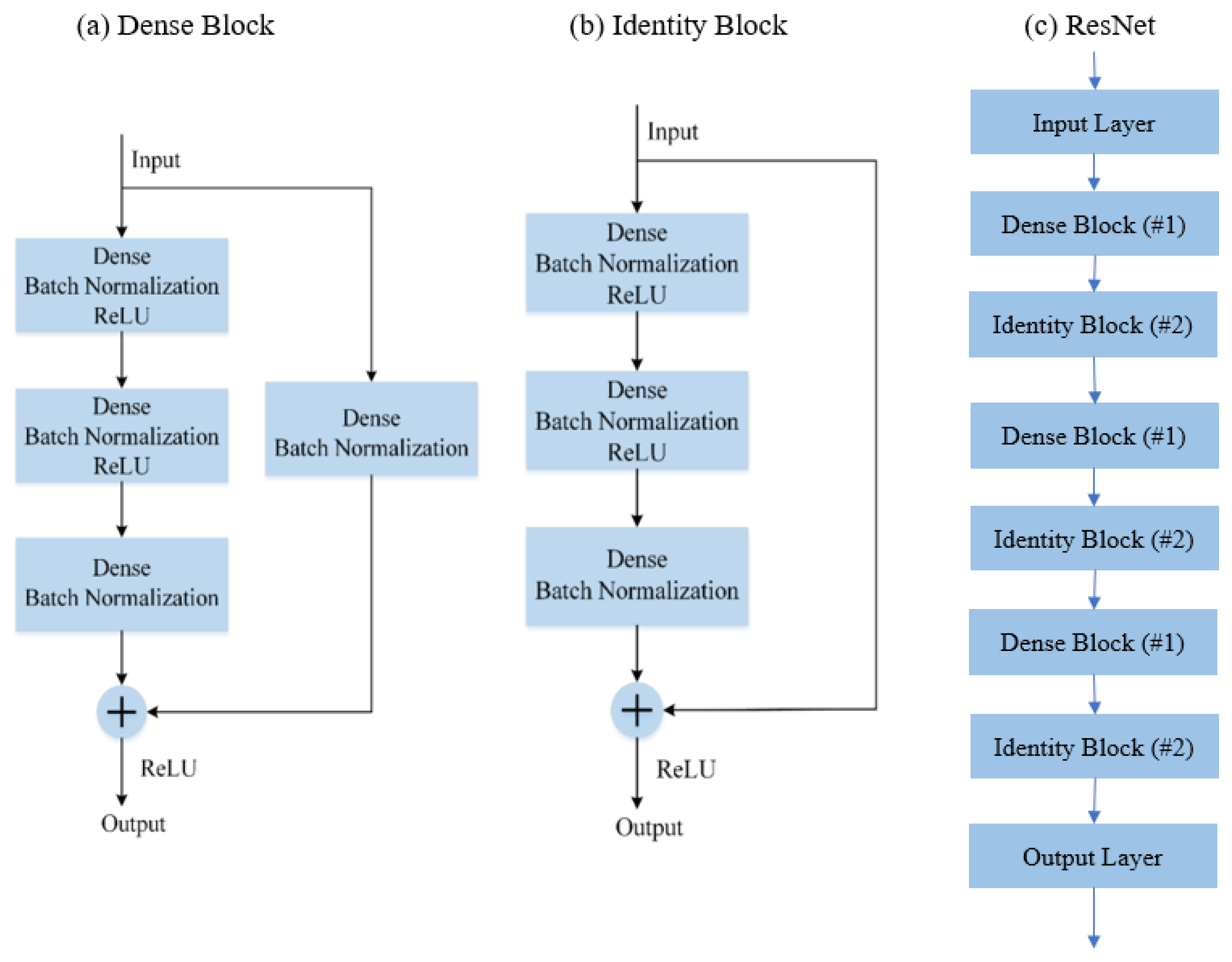
16], a neural network based model known as ResNet [
17]. To improve the result of creatinine prediction, we averaged results from eight predictors as our ensembling learning. Finally, the predicted creatinine and the original 23 features are used to predict the risk of CKD in a binary way.
The paper is organized as follows. In
Section 2, we describe the dataset and elaborate highlights of the experiment.
Section 3 describes the proposed method. The experimental details and results are discussed in
Section 4. The paper is concluded in
Section 5 with some ideas about the future direction of the work.
3. Proposed Methodology
Figure 4 shows two methods of predicting CKD Risk. In
Figure 4a, we predict CKD risk directly, and in
Figure 4b, we predict creatinine first and then combine its value with 23 features to predict the risk of CKD. The complicated nonlinear prediction of creatinine in model (b), make the input to CKD classifier richer in information. Compared to model (a), model (b) can achieve better classification. In this work, we used model (b) for CDK risk prediction.
In
Section 3.1, the preprocessing method of the data is described. To overcome the problem of imbalance in data, we used undersampling, which is described in
Section 3.2. We introduce a new cost-sensitive loss function in
Section 3.3. Finally, the model ensemble strategy is explained in
Section 3.4.
3.1. Preprocessing Method
In the preprocessing part, we did data cleaning as described in item (i) and item (ii) below. We also modified coding of some attributes as described in item (iii).
- (i)
Some samples have missing values on some attributes. As we already have a large data, 8654 samples with one or more missing attributes are removed.
- (ii)
There are some data with very large values of creatinine. Those samples are from patients at a late stage of renal failure. These subjects are not targets of this work, and therefore such data are classed as outlier data as far as training our target model is concerned. We removed 1234 samples with a value of creatinine higher than 2.5 mL/min.
- (iii)
In the original data, the attribute of Sex and SMK_STATE are not suitable for numerical coding. We changed them into one-hot coding format. We remove original variables and replace them with new binary variables where 0 is the value when the category is false and 1 when it is true. For example, sex is replaced by Male and Female, two attributes. For a Male subject, Male attribute is assigned a value “1” and female as “0”.
After preprocessing, 990,112 samples remained. We split it into a training set with 900,000 samples and a test set with 90,112 samples.
3.2. Undersampling for Data Balancing
3.2.1. Extremely Unbalanced Data
The distribution of target variable of creatinine is shown in
Figure 5. Most of the samples are concentrated near the median, and the number of samples away from the median is very less. A machine learning model will fit better on the region with more samples and perform worse around the region where data is less. In another words, the confidence interval of prediction accuracy will be wider where the samples are less.
For general regression tasks, the problem of unbalanced data can be ignored. If an interval contains less samples, we can say that the samples in that range are outliers. However, for this task, it is the opposite. Our target is to correctly predict those people who have a high creatinine value, though we have a few data for that range. From
Figure 5, we observe that most samples are between 0.5 and 1.4. If we use the whole dataset to train a machine learning model, as the training algorithm will try to minimize the sum error for the whole dataset, samples with high creatinine value where data is less will be ignored.
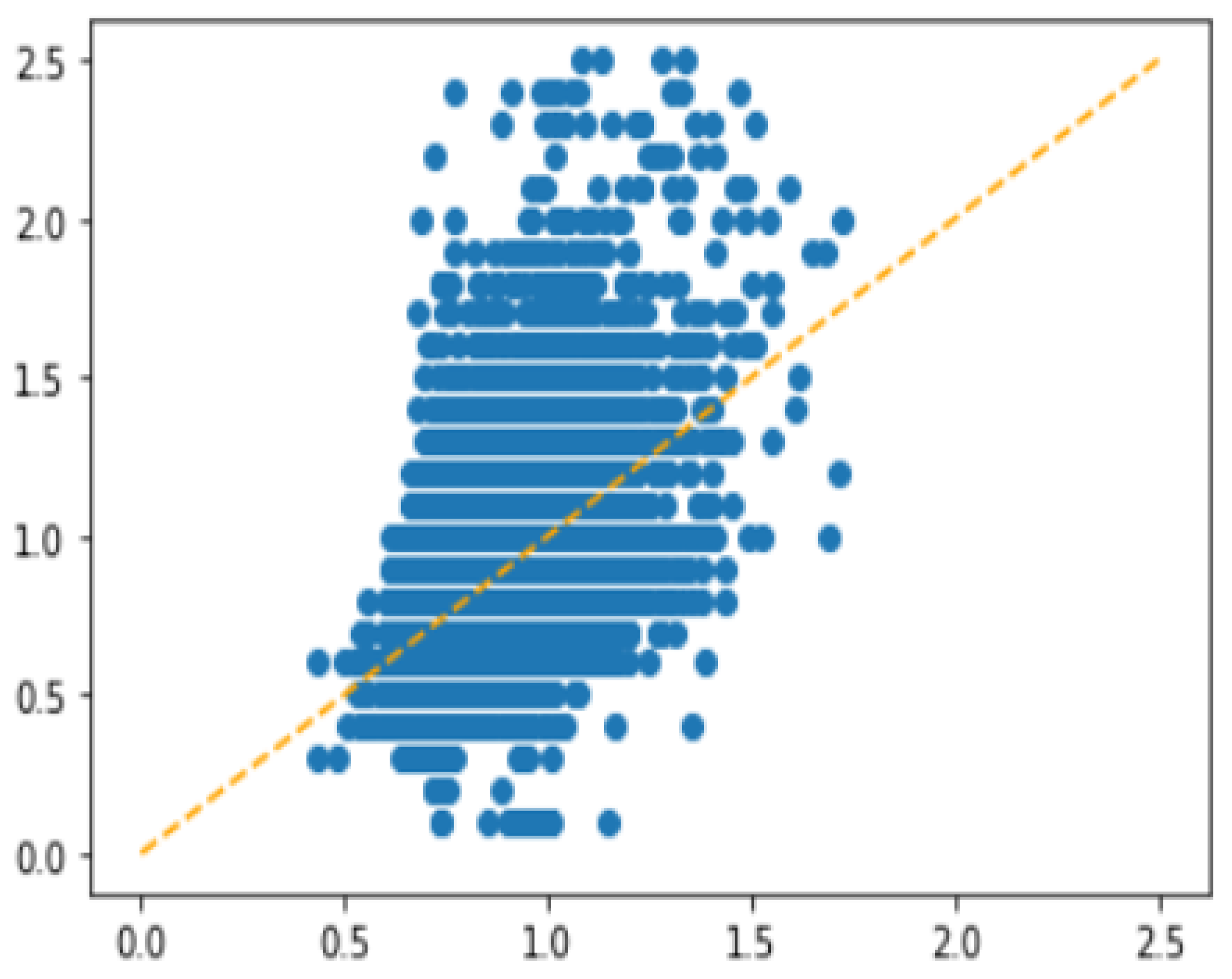
In order to show the impact of imbalance problem on regression more explicitly, we performed a simple experiment using XGBoost with Minimum Square Error (MSE) as loss function. The result is shown in
Figure 6, where the
y-axis represents the ground truth and the
x-axis is the predicted value. We observed that the model failed to predict for the interval with less training samples.
Generally speaking, the problem occurs because the number of samples with a high creatinine value is not enough for the machine learning model to learn from them. The data imbalance problem usually can be solved by data level methods and model level methods [
19]. Oversampling is the most common data level method. However, this data is obviously not suitable for oversampling. Over-sampling refers to balance data distribution by resampling or generating new data from low number of available ones. In this problem, high creatinine data is extremely low. Oversampling will cause noise in the rare data to be amplified countless times. We used undersampling method and proposed a cost-sensitive mean-squared error (MSE) loss function to deal with this problem.
3.2.2. Details about Undersampling
The target of the prediction, the creatinine value, is highly imbalanced in the data set. To alleviate the imbalance problem, undersampling is done on a range of values where a large amount of data is available.
Table 3 shows the details about undersampling. Six types of undersampling strategies are considered with different levels of undersampling as shown in
Table 3. Training data is more balanced as we go from sampling-1 to sampling-6. Total training data, shown in the last row of
Table 3, were 191,312, 107,439, 61,757, 34,220, 18,896, and 11,069 samples, respectively. As we opt for a more balanced set, the number of training data decreases. We performed experiments with all 6 sample sets and compare the results.
3.3. Cost-Sensitive MSE Loss Function
Mean absolute error (MAE) and mean squared error (MSE) are the two basic evaluation methods for regression tasks. Their formulas are shown below,
where
is the target value of the
labeled data, and
is the predicted value of the same from the regression algorithm. Errors in MSE are squared; it makes samples with small error less important (due to squaring) and creates a stronger incentive to train data with larger error. This happens for attribute values where the available data are rare. However, it does not mean that cost function with further higher-order on errors will achieve better results. Especially for data with noise which will be amplified too. In order to strike a balance, MSE is considered as a suitable loss function for this task.
Although MSE makes less frequent data more important, due to the imbalance of data, the model is trained to reduce error for more abundant data. This causes the error of the rare data to be larger than the common data. To alleviate this problem, we split the data into
k subsets. Then, calculate the mean error of each subset named as
and their average named as
. The ratio between
and
is used as a weight for the error of each sample from different subset. As the weight of error is sensitive to the cost of each subset, we called the loss function as cost-sensitive MSE, and its formula is shown as below.
Compared to the original MSE cost, we added a weight to the squared error for each sample. The weight is the ratio of and . This new loss function is implemented as follows.
- (a)
Calculate the range of target variable (Range) and minimum value of target variable (Min).
- (b)
Split the data into 10 subsets depending on Range. For example, samples with target variable larger than (0.2 × Range + Min) and smaller than (0.3 × Range + Min) belong to subset_3.
- (c)
After the first training epoch, calculate the mean error of each subset, which is named the .
- (d)
Calculate the mean value of for 10 subsets, which is the .
For the subsets with fewer samples, will be larger than and weight coefficient will be larger than 1. For the subsets with more samples, will be smaller than and weight coefficient will be smaller. Unlike using higher order exponential on errors, which is applied on all samples, the method we proposed is tuned for samples in specific intervals. The advantage of this method is that it can not only increase the importance of rare data, but also avoids the negative effects from high-order exponential errors applied to all samples in the training data set.
3.4. Model Ensemble Strategy
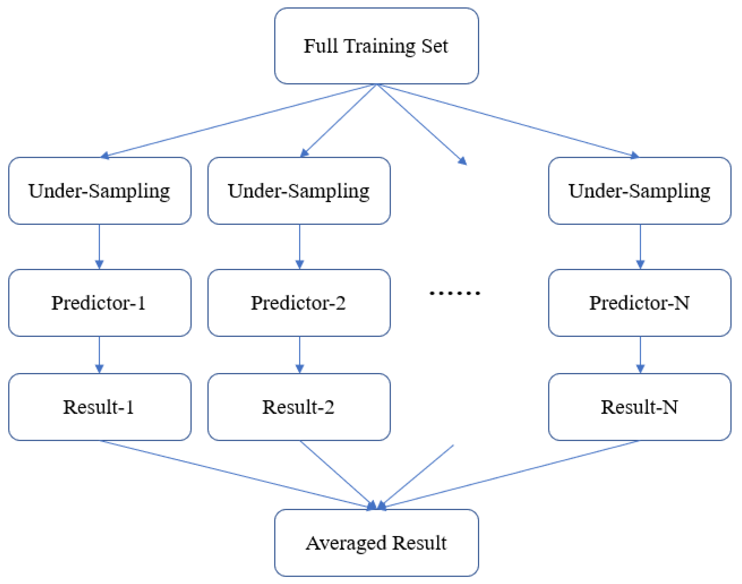
As undersampling method is used for data balancing, only a small part of samples are used for training. In order to better utilize the training samples, the model ensemble strategy is used as shown in
Figure 7. It is a bagging method that uses different sets of undersampled data and trains multiple predictors. Finally, the results from multiple predictors are averaged to improve generalization performance of the predictor.
5. Conclusions and Future Work
This study aims to build a regression model to predict the value of creatinine, then combine the predicted value of creatine with the common 23 health factors to evaluate the risk of CKD. As the creatinine value, which is the target variable, is extremely unbalanced, we used an undersampling method and proposed a cost-sensitive mean squared error (MSE) loss function to deal with the problem. Regrading model selection, we used three machine learning models: a bagging tree model named Random Forest, a boosting tree model named XGBoost, and a neural network based model named ResNet. To improve the result of creatinine predictor, we averaged results from eight predictors and ensembled their results. The ensembled model showed the best performance of R2 0.5590. The top six factors that influence creatinine are sex, age, hemoglobin, the level of urine protein, waist, and habit of smoking. With the predicted value of creatinine, an area under Receiver Operating Characteristic curve (AUC) of 0.76 is achieved when classifying samples for CKD.


