Inverse Multiscale Discrete Radon Transform by Filtered Backprojection

Featured Application

The startup company Wooptix is using the inversion by filtered backprojection of the multiscale Radon transform to accelerate inverse problem solutions in the context of wavefront phase optical measurements and barcode detection.

Abstract

The Radon transform is a valuable tool in inverse problems such as the ones present in electromagnetic imaging. Up to now the inversion of the multiscale discrete Radon transform has been only possible by iterative numerical methods while the continuous Radon transform is usually tackled with the filtered backprojection approach. In this study, we will show, for the first time, that the multiscale discrete version of Radon transform can as well be inverted with filtered backprojection, and by doing so, we will achieve the fastest implementation until now of bidimensional discrete Radon inversion. Moreover, the proposed method allows the sacrifice of accuracy for further acceleration. It is a well-conditioned inversion that exhibits a resistance against noise similar to that of iterative methods.

1. Introduction

The Radon transform is of great importance in the field of medical imaging and in general in problems where a magnitude cannot be directly sensed, and instead what is available is the magnitude integrated along a line, in which a beam of energy interacted with the physical medium [1,2].

Direct Radon transform performs integrals along lines while the inverse Radon transform takes the values in the transformed domain and must find out what values of the measure domain gave place to these already integrated values. This is a much harder problem to solve, as there may be many or no solutions (in the presence of noise), which makes the reverse path notably more complicated than the direct path.

Discretization is necessary at some point when using computers for solving the Radon transform pair. The projection-slice theorem or Fourier-slice theorem links the Radon transform with the Fourier transform, and has made it possible to solve the inverse Radon transform by means of the so-called filtered backprojection method. This method consists of placing Radon angular projections as one-dimensional slices of the Fourier bidimensional transform domain, then performing the inverse Fourier transform to finally obtain the bidimensional Radon inversion after high pass filtering has been applied [3].

Although this is the most common approach, an alternative method for computing the direct Radon transform was developed in the 90s [4,5,6]. It is known as the discrete multiscale approach of the Radon transform (DRT) and it avoids the use of Fourier transform, so it can operate only with integers. This transform, however, lacked an inverse algorithm until recently. In 2006 it was demonstrated by Press that this discrete version of the Radon transform has a fast and exact inverse, although iterative, using a multigrid method [7].

The purpose of this work is to demonstrate that it is possible to anti-transform the discrete multiscale version of the Radon transform using a filtered backprojection. With this goal in mind we pursue to obtain an exact algorithm that is faster than the already existing methods: those based on the Fourier-slice theorem and the Press’s discrete iterative inversion. And since the filtering is the computationally most expensive part of the method we will additionally characterize imprecise solutions that can be used to get approximated solutions, even faster.

1.1. Multiscale DRT

Multiscale approach of the discrete Radon transform was proposed at the end of the 90s by three groups of authors almost at the same time [4,5,6]. It is characterized by having a linearithmic complexity and does not use interpolation. It uses a divide-and-conquer approach and a definition of discrete line that avoids multiplication by non-integer values, which are substituted by logical AND interactions at bit level. This gives place to a transform that is performed multidimensionally, a bit at a time, similar to the Fourier transform: which, indeed, can also be interpreted as a divide-and-conquer transform that has linearithmic complexity.

In the continuum, the 2D Radon transform allows the description of a 2D signal, $f(·)$, in terms of the integrals along lines parameterized by an angle and a displacement, $(\theta ,\rho )$, instead of single values accessed by their horizontal and vertical pair of cartesian coordinates, $(x,y)$. This is,

$$\mathfrak{R}f(\theta ,\rho )=\int \int f(x,y)\delta (x·cos\theta +y·sin\theta -\rho )\mathrm{d}x\mathrm{d}y,$$

(1)

or, equivalently, using the absolute slope and displacement form, with $\left|s\right|<1$,

$${\mathfrak{R}}_{\left|\theta \right|\le \frac{\pi }{2}}f(s,d)=\int f(u,u·s+d)\mathrm{d}u,{\mathfrak{R}}_{\left|\theta \right|\ge \frac{\pi }{2}}f(s,d)=\int f(u·s+d,u)\mathrm{d}u.$$

(2)

The calculation of the Radon transform on a computer must deal with the discretization of data. Basically, for regularly spaced discrete data, they will be available only for a finite number of samples normally accessed with integer indexes. And the problem arises when the continuous definition of line integral makes necessary to evaluate the function at positions where there is no sample available and interpolation is required.

Götz & Druckmüller [4], Brady [5] and Brandt & Dym [6], almost simultaneously, proposed a divide-and-conquer approach reminiscent to FFT, in the sense that it works solving the problem at smaller scales and then combines those solutions to solve at greater scales, but with no multiplications nor complex twiddle factors involved, relying exclusively on integer arithmetic to achieve its goal. By working at multiple scales, and due to the symmetry of the problem, intermediate computations can be reused preventing any sum to be computed twice and so reducing the computational load from O($N^3$) to O($N^{2}logN$).

To make this possible, the key is to define a loose discrete line that traverses the domain visiting only integer positions, and therefore not exactly in a straight way. Ascensions are defined recursively, making lines composed of two halves, which in turn come each from other two-line segments of half their size and so on until line segments that join only two points are reached, and the problem cannot be further reduced.

DRT authors omitted to establish any sort of trigonometric relation between x and y variable, instead they decomposed u and s variables of Equation (2) into binary indexes and mixed them at binary level, one index of u and one index of s at a time, this way avoiding direct multiplication of u by a slope which would have produced non-integer indexes.

This can be achieved thanks to a loose definition of a discrete line, as follows:

$$l_s^n(u_0,\dots ,u_{n-1})=l_{\lfloor s/2\rfloor }^{n-1}(u_0,\dots ,u_{n-2})+u_{n-1}·⌊\frac{s+1}{2}⌋=\sum _{i=0}^{n-1}{u}_{n-1-i}·⌊\frac{⌊\frac{s}{2^i}⌋+1}{2}⌋$$

(3)

with $\lambda (u_0,\dots ,u_{n-1})={\sum }_{i=0}^{n-1}{u}_i·2^i$, i.e., the function that converts from binary multidimensional indexes, to decimal unidimensional index. This function l indicates how much ascends a line of slope s in a domain of size $2^n$ by the time it reaches position $\lambda (\mathbf{u})$. A digital line will be formed be the succession of points $\left\{(x,l_s^n(x))\right\},x\in \{0...2^n-1\}$.

With that definition it is possible to account for all the discrete lines of length 4, if we have previously computed all the lines of length 2. And so on. The definition of partial transform up to stage m emerges:

$$\stackrel{\sim }{f}{}^m(\stackrel{\mathbf{s}}{\overbrace{s_{n-m},\stackrel{\sigma }{\overbrace{s_{n-m+1},\dots ,s_{n-1}}}}}|\stackrel{\mathbf{v}}{\overbrace{v_m,\dots ,v_{n-1}}}|d)=\sum _{\mathbf{u}\in {\mathbb{Z}}_2^m}f(\lambda (\mathbf{u},\mathbf{v})|l_{\lambda (\mathbf{s})}^m(\mathbf{u})+d)$$

(4)

The integration variable, u (x if what we are considering are the horizontal lines), is now split in two, since we are transforming bits that go from being considered ‘vertical bands’, v, to being considered ‘slopes’, s. See Figure 1.

And finally, we arrive to the core equation that becomes the algorithm of the forward multiscale DRT, the equation that maps values from one stage to its consecutive:

$$\begin{array}{c}\hfill \begin{array}{cc}\hfill \stackrel{\sim }{f}{}^{m+1}(\underset{nbits}{\underbrace{\stackrel{\mathbf{s}:m+1bits}{\overbrace{s_{n-m-1},\stackrel{\sigma :mbits}{\overbrace{s_{n-m},\dots ,s_{n-1}}}}}|\stackrel{\mathbf{v}:n-m-1bits}{\overbrace{v_{m+1},\dots ,v_{n-1}}}}}|d)=\stackrel{\sim }{f}{}^m(\sigma |0,\mathbf{v}|d)+& \stackrel{\sim }{f}{}^m(\sigma |1,\mathbf{v}|d+s_{n-m-1}+\lambda (\sigma ))\hfill \end{array}\end{array}$$

(5)

Notice that single comma (,) is used to separate binary indexes, and vertical bar (|) is used to separate different parameters. This latter equation, surrounded by a for $m=0$ to $lo{g}_2(N)$ loop, and the adequate loops traversing variables $d,s$, and v is basically the forward DRT algorithm. It can be seen that it is performing just two sums to compute a new datum. The described outer loops account for the computational complexity: $O(N^{2}logN)$.

Notice also that the number of bits in partial stages is varying and depends on m, the current stage. When $m=0$, the array $\stackrel{\sim }{f}{}^0(s|v|d)$ is really bidimensional, as variable s is still empty, so $\stackrel{\sim }{f}{}^0(-|v|d)$ maps directly to $f(x|y)$. And when $m=n$, the last stage, variable v will be emptied, and so $\stackrel{\sim }{f}{}^n(s|-|d)$ is the desired result $\mathfrak{R}f(s|d)$. That can also be appreciated by evaluating the definition of partial transform, Equation (4), for stage $m=n$: $\mathfrak{R}f(s|-|d)=\stackrel{\sim }{f}{}^n(s_0,\dots ,s_{n-1}|-|d)={\sum }_{u=0}^{N-1}f(u|l_{\lambda (\mathbf{s})}^n(u)+d).$ This last equation is none other than the discrete version of Radon transform as expressed in Equation (2) with multiplication with the slope substituted by discrete line interaction between u and s at binary level.

More details on the formulation of the discrete Radon transform can be found on a previous work [8].

1.2. Inverse DRT

In contrast to the Fourier transform, the inversion of the algorithm does not invert the transform. In this case the algorithmic inversion leads to the adjoint transform, also known as backprojection.

The mapping formula that gives rise to its algorithm being:

$$\stackrel{\backsim }{f}{}^m(\sigma |v_m,\mathbf{v}|d)=\sum _{s_{n-m-1}}^{0,1}\stackrel{\backsim }{f}{}^{m+1}\left(s_{n-m-1},\sigma \left|\mathbf{v}\right|d-v_m·\left(s_{n-m-1}+\lambda (\sigma )\right)\right).$$

(6)

Since the data were summed in the direct method, the algorithmic inversion is only able to return an averaged version of the measured values in the original domain. Bringing them back to the locations where they were taken from does not undo the addition. In any case it prepares the data to apply a filtering that will undo the averaging, the smearing. The inversion proposed by Press does not make use of these terms, but the terminology inherited from the iterative methods of improving a solution of a system of equations.

In Press method, the exact inverse transform is unknown, but the adjoint transform is used as an approximation of it. In the loop that is formed by the direct and adjoint operators we know the application of the direct operator on the initial domain and the data in the transformed domain. By using backprojection as an approximated inverse operator, the error can be eliminated iteratively although the convergence is slow. Therefore, Press proposes to accelerate the convergence by using a multigrid method working in several scales. Even with that ‘acceleration’ a typical solution requires around 10 iterations to reach a 10e-3 normalized RMS error. Each iteration consists of ${log}_2(N)$ DRT pairs, i.e., a DRT pair at each scale below the original input size, $N\times N$. We will look for a more straightforward approach.

1.3. Initial Idea

The notion of directly deconvolving the backprojection of a multiscale DRT has not been applied until now. We initially thought that the reason was that the system formed by the direct DRT operator together with the adjoint operator is clearly nonlinear time-invariant (LTI), due to the different footprint around data that is located near the corners of the image, with respect to those that are located centered, see Figure 2. We have been able to solve this inconvenient with the idea presented in the next paragraph.

Two cases are represented left and right. Both show an inner square and an outer one marked by solid lines, as well as a dashed square in between. Let the side size of the external square be three times the size of the internal one. Marked in blue is a point in the inner square and two lines of the set of many that will be backprojected through it, represented with dashed pattern. The inner square represents the original size of our images: this used to be where the DRT backprojects. The length of the backprojected lines within the inner square clearly differs depending on the position of the point. If we manage to make our backprojection algorithm extend the lines up to the outer square, three times longer than the original, the backprojected lines will match in both cases when considering the dashed square around the dot, which is twice the size of the original.

Therefore, our idea to be able to apply deconvolution, –equivalent to the filtering in the filtered backprojection in the Fourier-slice theorem methods–, consists of creating a backprojection algorithm that takes the original DRT transformed data and backprojects them to a domain that is three times bigger in each dimension. To complete this initial idea we must also study how to deconvolve in a size two times bigger than the original image in each dimension. In the next section we will go into more detail in each of these two ideas: the extension of the backprojection to a three times bigger domain; and the characterization and deconvolution of the impulse response that is generated by the direct DRT and backprojection operators into a domain two times bigger.

2. Proposed Method

2.1. Extending Backprojection

It must be emphasized that the input data to our inverse transform will be the unaltered data that the conventional direct DRT provides. This data will be modified as little as possible: in fact, it would be more accurate, instead of using the term modify, to talk about rearranging those data to make them fit into a DTR four times larger.

We advanced previously that our goal is to make the backprojected lines grow up to three times the size of the input image. Therefore, any point in the original domain will have, in the extended domain, at least $(N-1)$ pixels of distance in straight line up to the new borders –being N the number of pixels of the input image–. This condition will make it possible to later deconvolve using 2D kernels of size $(2·N-1)\times (2·N-1)$.

Although our goal is to have at the lines backprojected to at least three times the initial size, actually we will make them grow to four times their original length. Because the algorithm works bitwise, we will grow by two bits the size of the image to keep it a power of two (that is $4\times$ bigger per dimension), then we will simply ignore N elements at each dimension (becoming $3\times$ bigger per dimension), as shown in Figure 3.

The initial domain of the image is shown in the inner square in Figure 3. Four lines of slope 0, 1, 2 and 3 are drawn through the upper right corner of said square. Marked in green are the points that intersect the left edge of the original image-square. Two squares that are three and four times bigger than the original, are also drawn. Marked in blue are the intersection of the same lines of slopes 0 to 3 in the left edge of these squares.

To the right, top and bottom, are depicted the relative positions of transformed data of slopes s = 0 to 3. Green and blue determining if they pertain to the original or the extended domain, respectively. In the original DRT the lines with consecutive values of s are also deployed at consecutive values of decreasing d. In the case of having a DRT of side four times bigger, these data would not belong to adjacent slopes, but multiples of four, and the intersections would not happen adjacently neither, but they would fall into multiples of two.

This is the basic idea behind the extension of a DRT to four times its original size. It is not necessary to modify the direct transform nor its backprojection algorithms, but to reorder the data. The formula that allows that a backprojected point leaves exactly the same footprint inside the original domain, and as symmetrical as possible outside of it, is slightly more complex than what was described in the introduction as the basic idea, in order to deal with the annoyances of a three-fold extension in a bitwise algorithm. More details on Section 2.2.1. The actual reordering formula for each quadrant being:

$$\mathfrak{R}\mathfrak{4}f(4N+d-2·(s+(s\%2)),4·s+3·(s\%2))\leftarrow \mathfrak{R}f(d,s)$$

$s\%2$ represents the remainder of the integer division between the slope and 2, that is the least significant bit of the slope: $s_0$. The reordering of the data has an $O(N)$ complexity and an example can be observed in Figure 4.

2.2. Characterization of the Impulse Responses

The next step before inverting the direct Radon transform is to completely characterize the impulse response of the operator conformed by the direct transform together with the just defined extended backprojection.

The most favorable case would be that, regardless of the location of these impulses, the response would be the same, only shifted. In that case it would be a time-invariant system that if it were in addition lineal—which it is in our case—it would allow to be quickly deconvolved dividing by the Fourier transform of the impulse response.

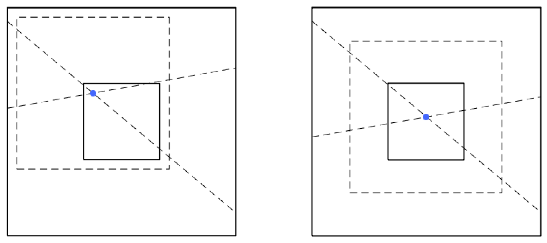
Unfortunately, the impulse responses change with the position in our case. The different responses are produced by how the different discrete lines travel the initial impulse depending on its position, because these same lines will be the ones that the backprojection transform returns. A single point—the isolated impulse to characterize—on the original image will be projected to exactly one displacement per angle, and will give rise to a line in the backprojection algorithm. All those lines ($4·N$, one per angle) will be backprojected and will intersect at the original point location. This accumulation of lines around the impulse will not be homogeneous nor the same in all positions of the input image because the definition of the lines yield non-straight lines.

The digital lines of the DRT are ‘broken’ lines (concatenation of line segments that approximate the line of desired slope) that avoid interpolation and that internally are the key to accelerate the algorithm since their recursive formula is fundamental to the divide-and-conquer approach. Therefore, it cannot be discussed if the non-uniformity of this lines can be relaxed, smoothed, as this is the heart of the method. The work that has to be done is to study how variable are these discrete impulse responses that the ‘broken’ lines give place to, and, in spite of this heterogeneity, how much the deconvolution can be accelerated even though the system is not properly LTI. That study is carried out in the next section.

2.2.1. Time Variant Impulse Responses

As stated previously, the following are the recursive and non-recursive definitions of discrete line:

$$l_s^n(u_0,\dots ,u_{n-1})=l_{\lfloor s/2\rfloor }^{n-1}(u_0,\dots ,u_{n-2})+u_{n-1}⌊\frac{s+1}{2}⌋=\sum _{i=0}^{n-1}{u}_{n-1-i}·⌊\frac{⌊\frac{s}{2^i}⌋+1}{2}⌋.$$

For example, when $N=8,n={log}_2(N)=3$, a ‘discrete’ line of slope $s=5$, will traverse through points $\left\{(u,l_5^3(u))\right\}$ with $u=0...N-1$, i.e.: $\{(0,0)$,$(1,1)$,$(2,1)$,$(3,2)$, $(4,3)$,$(5,4)$,$(6,4)$,$(7,5)\}$.

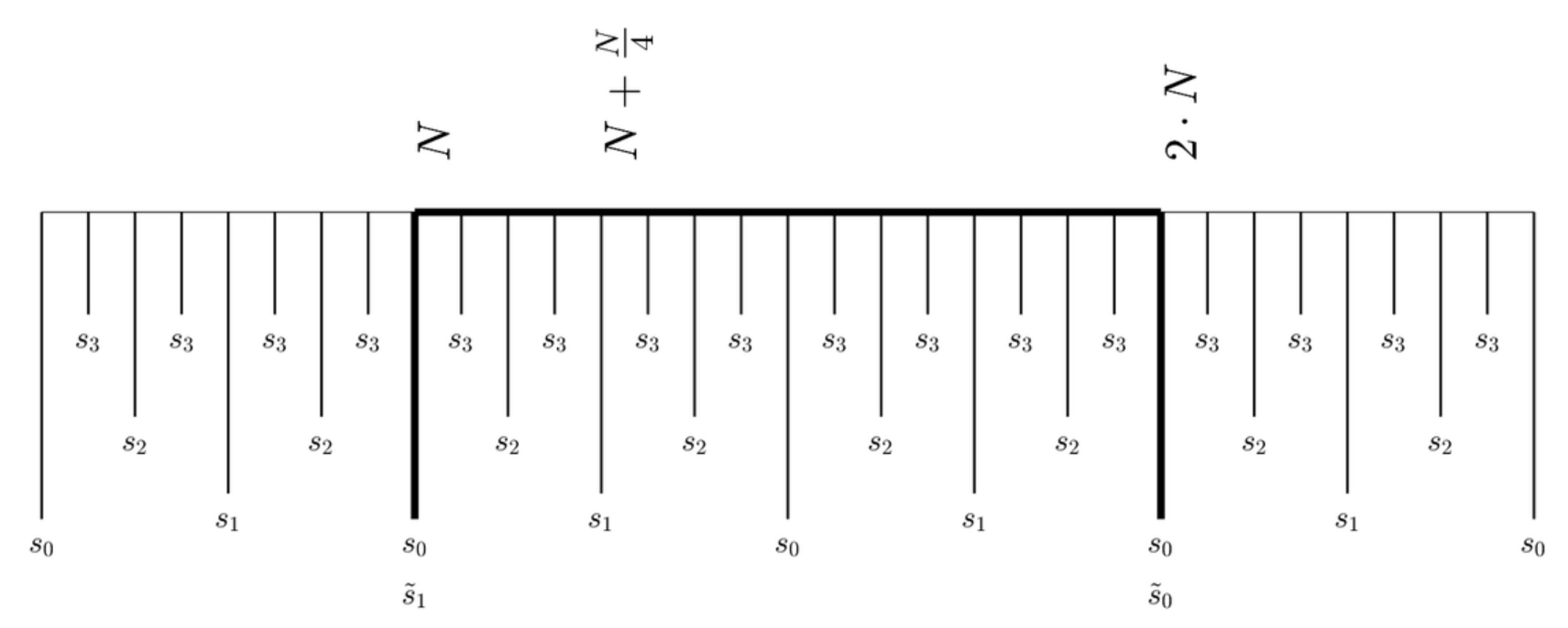
The lines with an odd ascent-slope will rise in the boundary between the values $N/2-1$ and $N/2$. This is the ‘bit boundary’ with the most significant bit weight: $2^{n-1}=N/2$. In other words, whether a line ascends or not preceding $N/2$ will be determined by the least significant bit of the slope, $s_0$ (which is one for odd numbers). The next least significant ‘bit boundary’ occurs at $N/4$ and $N/2+N/4$, and the ascent in there will be determined by bit $s_1$ of the slope. In general, the bit $s_i$ of the slope will determine whether to ascend or not at positions whose greatest power of two divisor is $2^{(n-1-i)}$. In the previous example, for $n=3$ and $s=5$, the discrete line has ascended in bit boundaries $s_0(u=3\leftrightarrow 4)$ and $s_2(u=0\leftrightarrow 1,2\leftrightarrow 3,4\leftrightarrow 5,6\leftrightarrow 7)$, and remained without ascension for $s_1(u=2\leftrightarrow 3,5\leftrightarrow 6)$; of course, in accordance with $s=5$ expression in binary as $(1,0,1)$.

The bits boundaries of the slopes for the extended DRT that we propose are shown in Figure 5. The N original data are located between positions N and $2·N$ when the domain is extended to $4·N$. The figure shows those positions, as well as $N/2$ additional values to each side.

An impulse that is located originally at the position 0 in one dimension, will be located at the position N in the extension and through it there will be N lines crossing, with slopes approximately equal to the multiples of 4 of the values from 0 to $N-1$. Actually, the original slopes were $s=0...N-1$, but now they will be $\tilde{s}=4·s+3·(s\%2)$; this means that we add 3 to the odd slopes. This process at bit level is equivalent to shifting two places to the left the original bits of the slope and replicate in the two least significant additional bits the original $s_0$ bit.

In the Figure 5 this phenomenon is highlighted in the boundaries around N and $2·N$, limits where the original image is placed in, and that in terms of the extended slope it would be flanked by the bits ${\tilde{s}}_1$ and ${\tilde{s}}_0$, but to the effects of the lines that we are going to inject in the system these bits are equivalent to $s_0$.

With this preamble we can move on to describe how the combined response of the direct transform plus the adjoint transform is configured around an impulse in any position of a dimension of an image. The following description will be valid for the quadrant of positive slopes. The negative slopes are a horizontally inverted replica of the responses we will characterize now. The responses in the other dimension can be found with a transposition.

The impulse response to a unitary input located originally in the position 0 (extended position N) in a problem of size $N=16$ will find in the positive horizontal direction and by order of boundaries: $s_3,s_2,s_3,s_1,s_3,s_2,s_3,s_0,s_3,s_2,s_3,s_1,s_3,s_2,s_3$, see Figure 5. If the size of the problem was, instead, $N=8$, the $s_3$ boundaries would not exist. If the size of the problem was $N=32$, there would be additional $s_4$ boundaries interleaved between those of the $N=16$ case, and so on. We will analyze the case $N=8$ for simplicity, and therefore the boundaries will be: $s_2,s_1,s_2,s_0,s_2,s_1,s_2$.

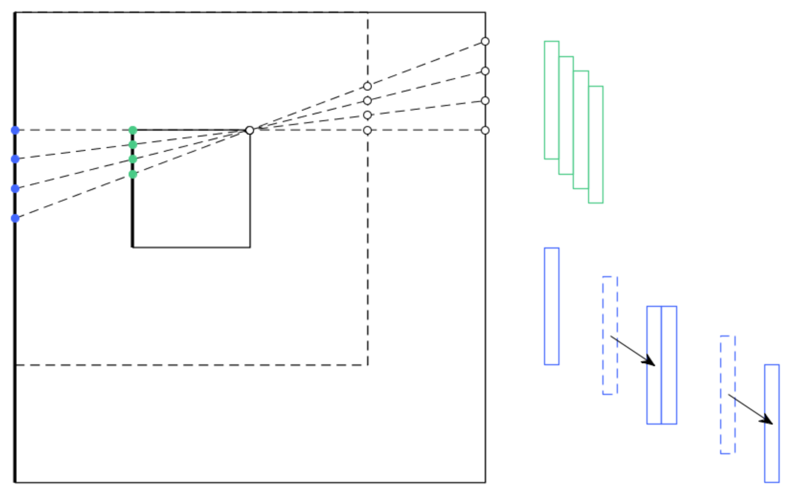
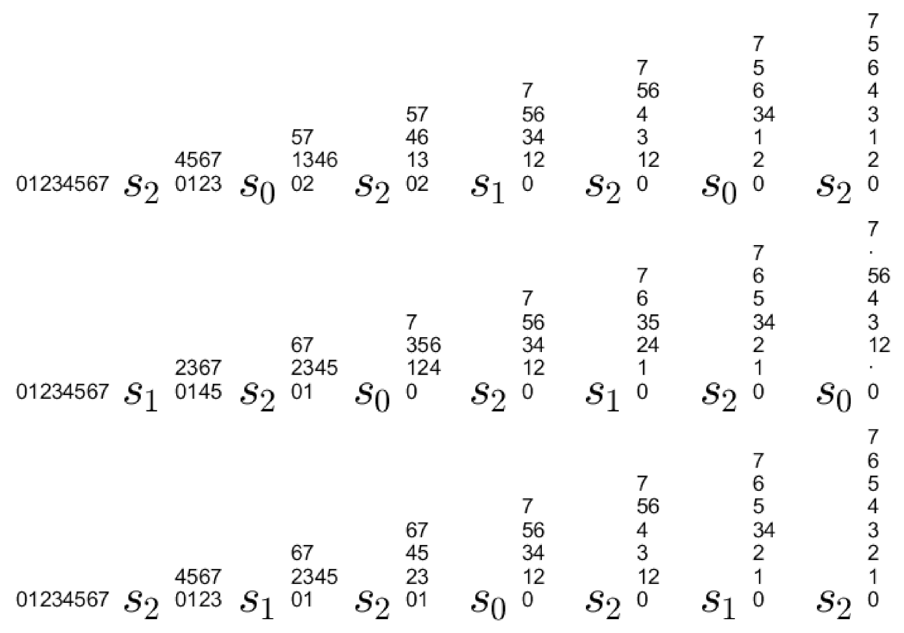
It is shown in Figure 6 how the lines of slopes 0 to 7 are distributed by height for three possible bit boundaries as they travel to their right. Those bit boundaries would be the ones that would cross the lines depending if the origin point was at position 0, 1 or 2, in a problem of size $N=8$.

In the case depicted at the bottom—corresponding to starting from position 0—the first bit boundary, $s_2$, breaks the group composed of the lines of slopes 0 to 7 into two groups: the lines with slopes 0 to 3 which do not ascend at that boundary, and the lines of slopes 4 to 7, that ascend because they have a 1 in the bit 2 of their slopes. The rest of the diagram can be interpreted in the same way. It can be seen that if we join the cells that contain each number from 0 to 7 with line segments we would obtain the 7 discrete lines of the DRT: lines that ascend in a ‘broken’ way but in an orderly fashion and that finish after traveling N positions to the right, having ascended what its slope determines: 0 to 7.

The shape of the impulse response will be determined by the number of lines that occupy each height at a certain distance, in this case, moving away from the starting point to the right (separated by square brackets) and ascending from height 0 (separated by commas inside the square brackets): $\left[8\right]$, $[4,4]$, $[2,4,2]$, $[2,2,2,2]$, $[1,2,2,2,1]$, $[1,2,1,1,2,1]$, $[1,1,1,2,1,1,1]$, $[1,1,1,1,1,1,1,1]$. For each distance u, we have u values that add to N which are palindromes.

Considering the intermediate case, which simulates an impulse at position 1 (extended N+1), is equivalent to thinking of the boundaries for case 0 shifting to the left, with the disappearance of a $s_2$ and the appearance of a $s_0$ from the right. The impulse response will change with respect to the previous starting position, and we obtain: $\left[8\right]$, $[4,4]$, $[2,4,2]$, $[1,3,3,1]$, $[1,2,2,2,1]$, $[1,1,2,2,1,1]$, $[1,1,1,2,1,1,1]$, $[1,0,2,1,1,2,0,1]$.

However, in the next position, 2 (extended $N+2$), although the bit boundaries change with respect to both cases 0 and 1, the impulse response is the same as in case 0. This is because the roles of boundaries $s_0$ and $s_1$ are interchanged with respect to that case, but given that the path that each line follows does not matter but the number of lines crossing at each height, the final result in terms of impulse response is the same.

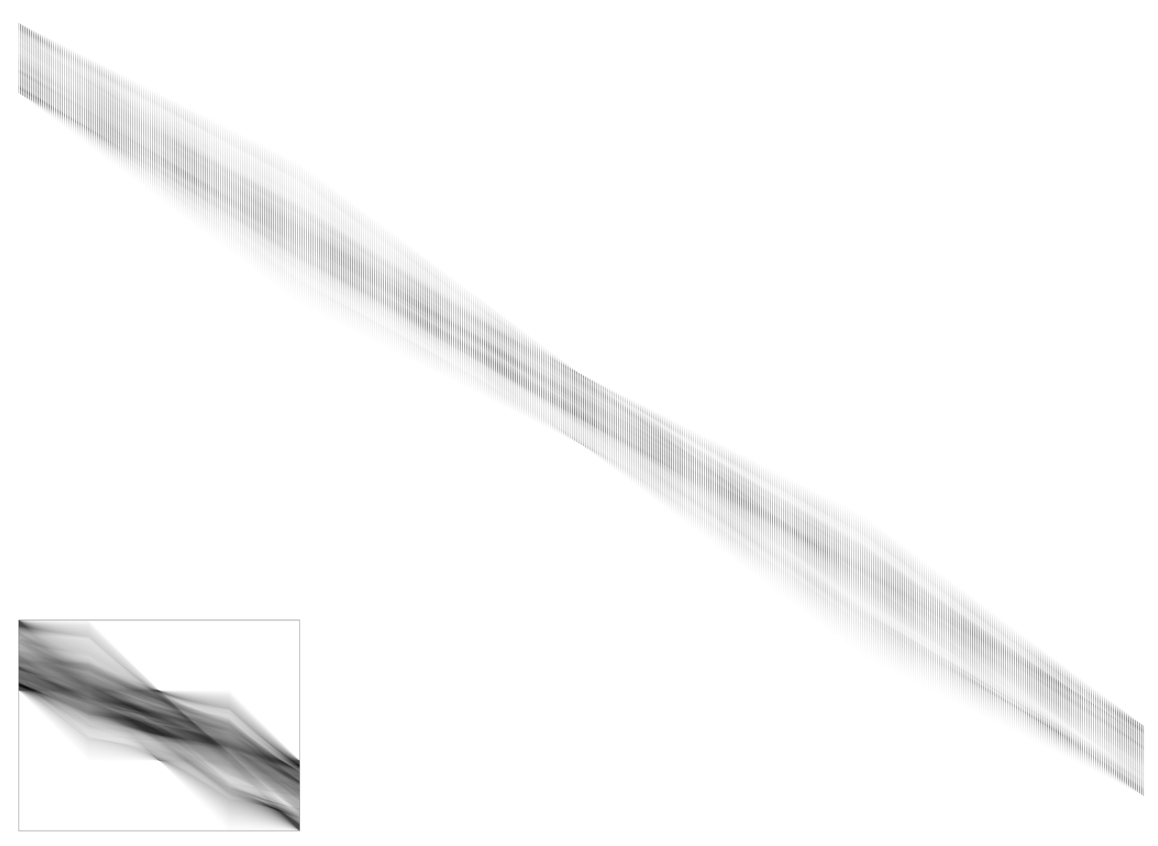
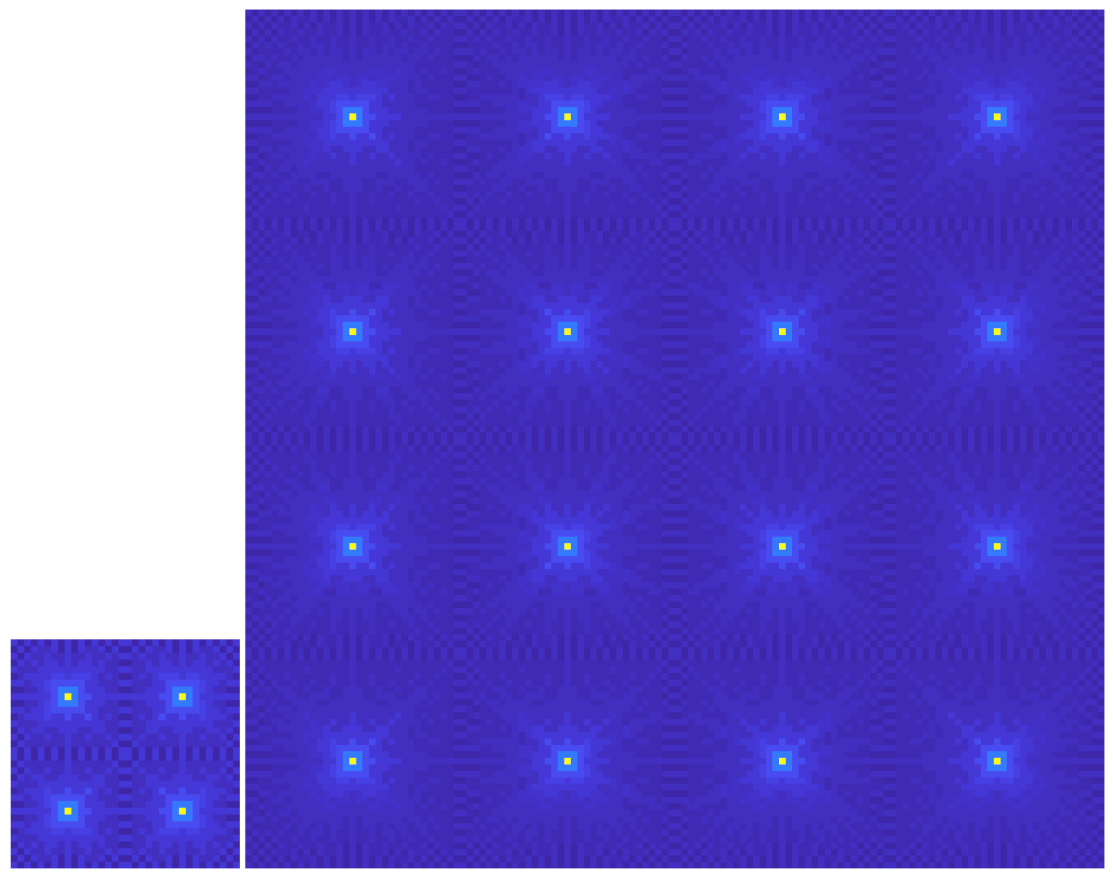
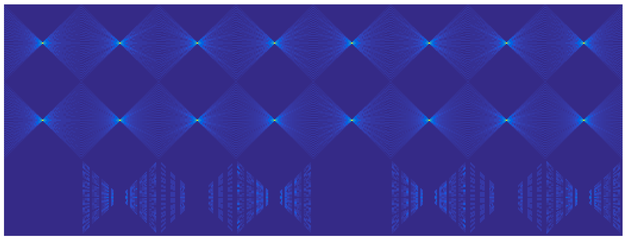
With the proposed adaptation from original slopes to extended ones, which replicates the two least significant bits of the slopes, we have managed to make the bits ${\tilde{s}}_1$ and ${\tilde{s}}_0$ equal to $s_0$, and therefore a periodicity appears after $N/4$ displacements of the impulse starting position. After N/4 shifts, the bit boundaries repeat, only that swapping the roles of bits $s_0$ and $s_1$. Therefore, the number of different impulse responses that we need to study will be $N/4$. They will have size $(2·N-1)\times (2·N-1)$, in 2 dimensions: this is, the central value will be surrounded by $N-1$ values on each side; and characterize half the impulse response (only in one dimension). They form a kind of ‘butterfly’ which is different from zero only in the positions closer to the horizontal axis than it is to the vertical one. Examples of this sort of ‘butterflies’ will be shown later.

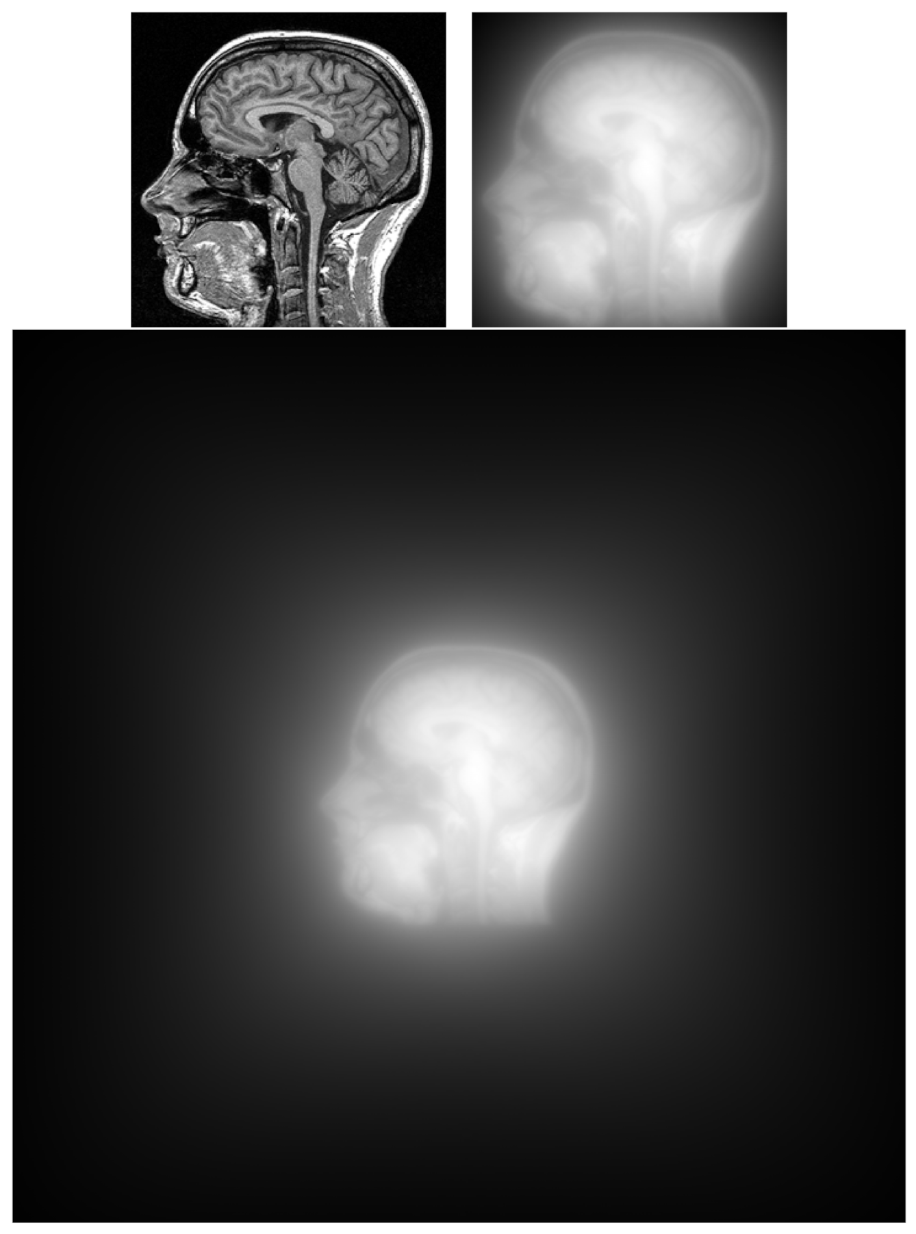
The total impulse response at position $(x,y)$ will be the sum of the horizontal half-impulse response $x\%(N/4)$ with the horizontal transposed half-impulse response $y\%(N/4)$, see Figure 7, with (%) representing the remainder of integer division. It would have been more desirable to have only one impulse response, but at least we do not have $N\times N$ different ones. 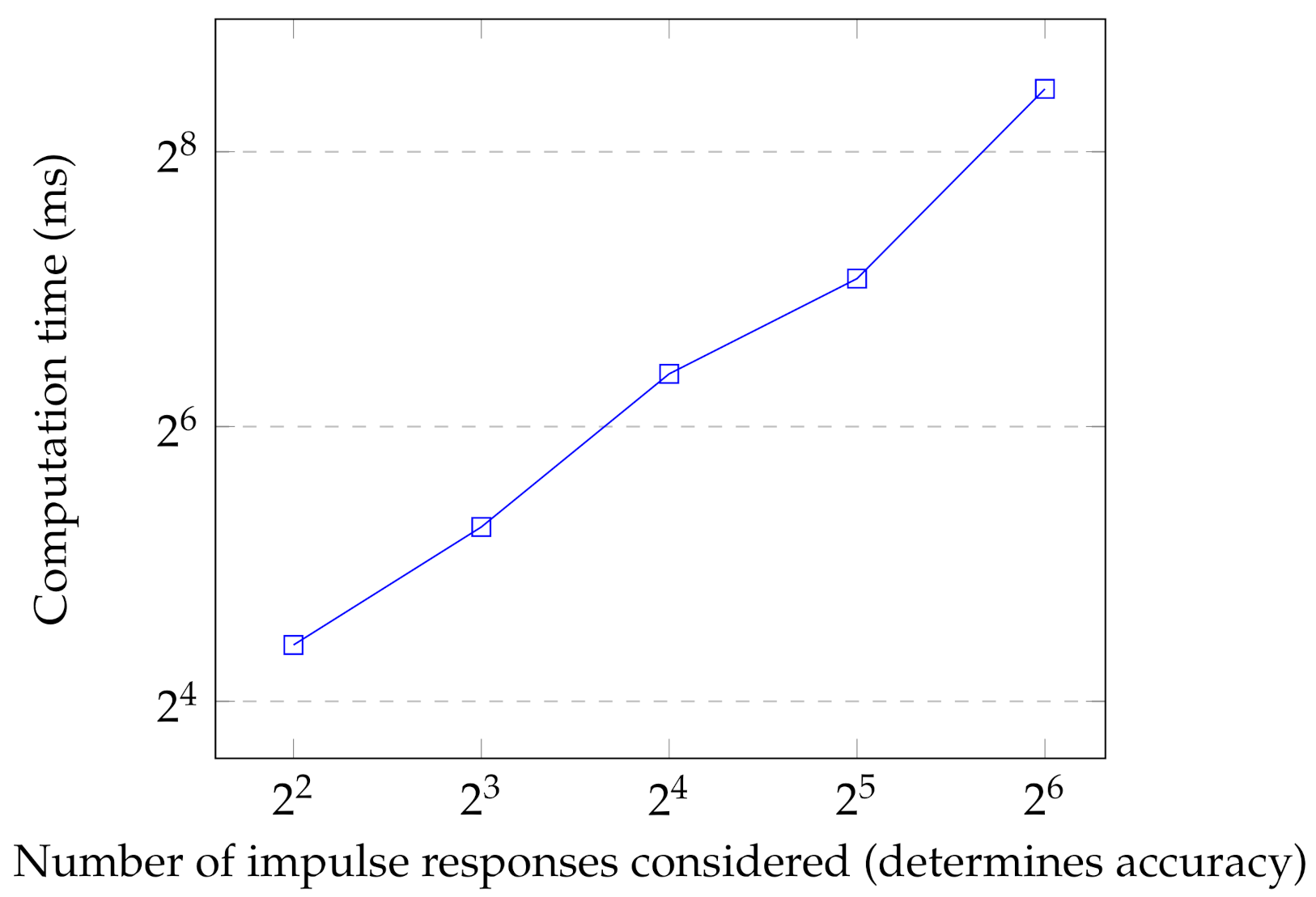We have $N/4\times N/4$, but can operate with $N/4+N/4$ different ones given that they can be decomposed into horizontal and vertical, where they are the transposed versions of each other. We will see later that we can even lower this number if we allow the sacrifice of fidelity in the reconstruction.

2.3. Deconvolving Different Impulse Responses

By using Fourier, we can only deconvolve quickly if all the positions generate the same impulse response, but that is not the case, as we have shown that we can have $N/4$ different impulse responses affecting the horizontal half and $N/4$ affecting to the vertical half of the vicinities of a point. Our task now is to create a method that takes into consideration this diversity of impulse responses. It works in our favor that the responses and the positions where they happen are known. We could say that this system is partially LTI: it is not completely LTI, but its variability is limited enough that it can be deconvolved with a couple of iterations of simple deconvolutions.

Let $f(x)$ be an unidimensional unaltered signal; and let $m(x)$ be the measured signal that results by altering $f(x)$ by some known finite impulse responses $q(x)$ or $r(x)$, each impulse response affecting respectively to samples at positions $P_q(x)$ or $P_r(x)$; those functions will be 1 where the system responds with the response q and r respectively, or 0 otherwise; and let $P_q(x)+P_r(x)=1,\forall x$. Then $m(x)=[f(x)·P_q(x)]*q(x)+[f(x)·P_r(x)]*r(x)$, the (*) symbolizes the convolution operand.

Let us denote the inverse of the impulse response $q(x)$, with $\tilde{q}(x)={\mathfrak{F}}^{-1}\left(\frac{1}{\mathfrak{F}(q(x))}\right)$, and let us use it to deconvolve the whole $m(x)$ signal. The values at positions $P_q(x)$ will be back, mostly, to their original values, ${f(x)|}_{P_q(x)=1}$, except for the tails of adjacent $r(x)*\tilde{q}(x)$ elements at positions $P_r(x)$ that are perturbing them: $m_q(x)=m(x)*\tilde{q}(x)=[f(x)·P_q(x)]+[f(x)·P_r(x)]*r(x)*\tilde{q}(x)$. The next step is to eliminate these perturbations with a second deconvolution only performed at position $P_r(x)$ with the compound of $r(x)*\tilde{q}(x)$. Let us denote by $r\tilde{q}(x)=(r(x)*\tilde{q}(x))$, and with $r\tilde{q}(0)$ the central value of that kernel. Then, it be can written:

$$f_0(x)=m_q(x)$$

$$f_n(x)=m_q(x)-{\left[f_{n-1}(x)·P_r(x)/r\tilde{q}(0)\right|}_{n=1}]*r\tilde{q}(x)+[f_{n-1}(x)·P_r(x)/r\tilde{q}(0){|}_{n=1}]$$

$$f(x)\approx f_n(x)n\to \infty$$

The subtracting term eliminates the wrongly deconvolved elements at positions $P_r(x)$, and their surroundings. Then we reincorporate our best guess, up to that iteration, just at the main spike of the kernel at those positions. Notice that the central value of the kernel may differ from one, so we are compensating this effect with the divisions by $r\tilde{q}(0)$, but only in the first iteration. For the sort of impulse responses that backprojection DRT generates, the just proposed method recovers $f(x)$ from $m(x)$ in 2 or 3 iterations, and can be easily extended to more dimensions and for more than two impulse responses.

3. Results

In Figure 8 a $256\times 256$ grayscale image is shown, its conventional DRT backprojection and the backprojection extended to a three times bigger domain. If we subtract one backprojection from the other, centered, we would see they are identical, as the method is designed so that the extended backprojection agrees with the conventional one in the original domain.

The next figure, Figure 9, shows what happens when we deconvolve the extended backprojection in Figure 8 with just one impulse response, incorrectly assuming the direct+backproject transforms can be treated as a LTI system. Artifacts of high frequency can be observed.

On the other hand, Figure 10 shows the application of the method described on Section 2.3 with 64 vertical + 64 horizontal impulse responses and two iterations.

In addition, as $N/4+N/4$ deconvolutions per iteration, even if there are only two iterations, may seem a lot of computations, we studied how similar are these impulse responses between them. In Figure 11 we show the recovery when using less than the required $64+64$ impulse responses. In order to reduce the different impulse responses we have applied a k-means clustering algorithm with norm-2 distance, and averaged the impulse responses within the same cluster, see Figure 12.

In our tests we have found a good balance to be $N/16$, in this case $16+16$ impulse responses (top right image), as for several images we have obtained PSNR of around 30 dB, independently of N, with that trade-off ($N/16$ instead of $N/4$). The execution times are presented in Figure 13. Notice that both axes are on log 2 scale.

4. Discussion

Our method is compared in this section with two alternative algorithms that compute the inverse Radon transform. One represents Fourier-based methods that we will name after the author of the software package: Shkolnisky [9,10,11,12]; another represents the only method currently available for inversion of the multiscale DRT: that due to Press [7]. These methods are compared with ours in terms of processing time, for the same quality target of 30 dB PSNR, and on the same machine, a PC with an intel i9-9900K processor running at 3.60 GHz, with implementations as optimal as possible. Performance was measured in the same conditions for all algorithms and averaged for several executions.

Our method will be measured with the number of impulse responses $K=N/16$. For the image of reference, Figure 11, the method from Press requires 6 iterations to get the same level of quality. Shkolnisky’s method needs 5 iterations to obtain a similar PSNR.

Our extended backprojection algorithm was implemented in Halide language [13], and the convolutions in the Fourier domain in OpenCV, compiled specifically to the selected processor using intrinsics functions. Convolutions were computed in parallel using the 8 cores-16 threads of that CPU. The code provided by Shkolnisky [12] is parallelized and uses effectively the 8 CPU cores. Press’ method was implemented by us in Python using Numpy to use optimized, parallel, matrix-vector functions, and Cython when needed, obtaining C compiled code to avoid memory copies in Python.

Figure 14 shows the comparison between the different algorithms. For every image side size in the comparison, from 64 to 2048, our proposed method is systematically faster than the other two methods. The speedup is approximately $3x$ in comparison with the second fastest method. But depending on the size and method with which we confront it, the speedup can be more than ten times greater.

Figure 15 shows how the different methods react when there is noise in the transformed domain. The recovery that our proposed method achieves coincides completely with Press’ inversion. Although visually there is a difference in contrast with Shkolnisky’s method, the PSNR tell us the fidelity of reconstruction falls in the same proportion (from 30 dB to 15 dB) when we add a similar quantity of gaussian noise in the transformed domain.

5. Conclusions

We have developed a method that explores a new way to invert Radon transform, which is appropriate to cope with images previously transformed with the multiscale approach of DRT. Before this contribution, the only method available was due to Press and prescribed an iterative multigrid method, or similar generic numerical methods as those of conjugate gradients. We have shown that there is a solution studying the impulse response of the direct transform combined with the adjoint transform, as a whole. Unfortunately this combined operator turns out to be non LTI, but still we have found it to be possible to deconvolve this combined operator as there are only $N/4\times N/4$ different impulse responses in a problem of size $N\times N$. Moreover, they are separable into $N/4+N/4$ known impulse responses, which will appear in equally known positions. The similarity between those impulse responses is such that perfectly fine inversions can be achieved with less impulse responses than $N/4+N/4$, so that we can sustain video-acquisition rate preview through Radon domain using this technique for some wavefront phase inversion problems, at 256 × 256 resolution just relaxing slightly the quality of the preview.

We plan to extend this method to Radon inversion in more than two dimensions [14] and as a tool for blind acoustic source localization [15].