Residual Stress Relaxation of DRWDs in OSDs under Constant/Variable Amplitude Cyclic Loading

Abstract

An orthotropic steel deck (OSD) has a complicated structure, and its fatigue life is mainly determined by various welding details. Fatigue assessment of deck-to-rib welding details (DRWDs) under long-term train loads is an important concern for engineers. Properly assessing the initial residual stress and the mechanism of stress relaxation in DRWDs under long-term external loading is a prerequisite for predicting the fatigue damage and service life of OSDs. In this paper, a finite element analysis method is proposed to calculate the residual stress relaxation in DRWDs of OSDs under constant/variable amplitude cyclic loading. First, experiments on full-size OSD specimens were carried out using the hole drilling strain-gauge method, and the multi-axial distribution characteristics of residual stress on the sub-surface of the deck were obtained. On this basis, a refined residual stress analysis model of DRWDs using thermal-structural sequence coupling analysis and life and death unit technology is established, and the accuracy of the model is verified by the test data. Second, a coupling stress analysis model that considers the welding residual stress and mechanical stress using cyclic plastic constitutive model is established. The combined influence of number of cycles, stress amplitude, and stress ratio on multi-axial residual stress relaxation effect under constant/variable amplitude cyclic loading is investigated. Finally, a release formula of welding residual stress relaxation coefficient is proposed based on the external loading stress amplitude, stress ratio, and material yield stress. The results show that (1) with the increase in the number of loading cycles, the stress decreases until it is stabilized, while the global distribution of welding residual stress remains unchanged. Most of the welding residual stress release (about 95%) occurs in the first cycle; (2) the residual stress relaxation decreases with the increase in stress amplitude and increases linearly with the stress ratio; (3) the residual stress release is controlled by the maximum amplitude stress in the variable amplitude cyclic loading. After the residual stress is released, the stress will not continue to be released if the DRWDs have the same or smaller amplitude loading.

1. Introduction

Orthotropic steel decks (OSDs) have been widely used as main girders in long-span bridges as a result of their high load-loading capacity, light weight, excellent aerodynamic, and speedy construction [1,2]. Recently, many fatigue cracks have been reported in OSDs in China and other countries. For instance, three types of fatigue cracks were found in the rib-to-deck welds on the Severn Bridge in the UK after the bridge was open to traffic for five years. Numerous fatigue cracks were observed in OSDs on the Second Van Brienenoord Bridge in Denmark after it was in service for seven years, which resulted in the bridge being difficult to repair. Fifteen years after the Rio‒Niterói Bridge was built in Brazil and opened to traffic, it was found that serious cracks of OSDs had developed, mainly distributed in deck-to-rib welding details (DRWDs). Serious fatigue issues have occurred in the Humen Bridge, the first bridge with OSDs in China, after it was in service for only five years. The Jiangyin Yangtze River Bridge, located in the Yangtze River Delta, the busiest transportation region in China, also had fatigue cracks nine years after construction [3,4]. Numerous cases indicated that the fatigue behavior of OSDs under long-term train loading is an important concern. The fatigue cracks in DRWDs appear most frequently among the various types of cracks in OSDs [5,6,7]. Moreover, it is difficult to repair and detect such cracks, which seriously affects the durability and safe operation of bridges.

The welding residual stress plays a vital role in the fatigue assessment of DRWDs. Welding, as a steel structure connection method, is widely used in the fabrication of OSDs. Therefore, it is inevitable that it will produce welding residual stresses owing to the local plastic deformation induced by the local high temperature during the welding process. The existence of high residual stress at the welding details will result in a significant decrease in the fatigue strength bearing capacity of the structure [8,9,10]. However, the initial welding residual stress in the structure might be relaxed under cyclic vehicle loading, which resulted in the variation of distribution and magnitude of residual stress around the welded joints [11,12]. Hence, the real stresses at the welding heat-affected zone under the coupling effect of residual stress induced by welding and mechanical stress caused by external loading cannot be determined, but they produce a lot of resistance to the fatigue damage assessment and life prediction of the pivotal welding details of OSDs. As a result, the relaxation effect of welding residual stress under cyclic loading should be taken into account in the fatigue strength analysis of OSDs. Researchers have studied the release behavior of residual stress in a simple welded structure under constant amplitude cyclic loading by experimental methods, and determined the calculation release formula of residual stress based on the experimental data [13]. Due to the high cost of experimental methods, the finite element (FE) method is introduced to analyze the relaxation behavior of residual stress. Dattoma et al. [14] and Wang et al. [15] simulated the release behavior of residual stress under constant amplitude cyclic loading by the 3D heat conduction elastic‒plastic method. In recent years, Chinese scholars carried out research on the influence of the welding residual stress on the fatigue life of OSDs [3,16,17], but few focused on the relaxation effect of residual stress. Cui et al. [18] studied transverse residual stress relaxation in innovative both-side welded rib-to-deck joints of OSDs under constant amplitude cyclic loading. Numerous studies have shown that the relaxation behavior of residual stress is a complicated process [19,20] affected by multiple variables, such as the stress amplitude, stress ratio, loading cycles, material properties, etc. However, it is worth noting that the vehicle loading is often a cyclic loading with variable amplitude. Unfortunately, all of the existing literature investigates the uniaxial residual stress relaxation of simple welded joints under constant amplitude cyclic loading, but seems to lack information on the release behavior of multi-axial residual stress under variable cyclic loading at the heat-affected zone of complex DRWDs.

In this paper, a FE analysis method is proposed to calculate the relaxation effect of the welding residual stress under the external cyclic loading of DRWDs in OSDs. First, a refined residual stress analysis model of DRWDs is established based on the element birth and death technology in the FE software ANSYS and the thermal-structure sequence coupling analysis method, and the initial distribution of transverse/longitudinal welding residual stresses are obtained. Then, residual stress tests of the full-size OSD specimen are carried out by using the hole drilling strain‒gauge method, and the accuracy of the FE model is verified by the test results. Second, a stress relaxation analysis model, which considers the coupling effect of the welding residual stress and external loading stress, is established on the basis of the cyclic plastic constitutive model. The influence of the number of cycles, stress amplitude, and stress ratio on the multi-axial residual stress relaxation effect under constant/variable amplitude cyclic loading is analyzed. Last but not least, a release formula of welding residual stress relaxation coefficient is proposed, which takes into account the factors of the external loading stress amplitude, stress ratio, and material yield stress. The research results may provide a technical reference for the structural design and fatigue assessment of this type of OSD.

2. Welding Residual Stress Distribution

2.1. Welding Residual Stress Measurement

An experiment on full-size OSD specimens was carried out to investigate the welding residual stress of DRWDs of a Q345 steel deck. In this study, the Jiangyin Yangtze River Highway Bridge, the first extra-large steel box girder suspension bridge with a span of kilometers in China, was taken as a case study. Thus, the structural style and dimensions of the specimen in this paper is made referring to the OSDs in main girders of this bridge. Figure 1 shows the cross section and dimensions of the OSD test specimen. It is seen that the specimen was 1200 mm long, 300 mm wide, and consisted of one top deck and two U-ribs. The thickness of the top deck was 12 mm, and the thickness of the U-ribs was 6 mm. The material of the specimen was steel of Q345 quality, which implies a yield strength (f_y) of 345 MPa. In the welding, CO₂ gas shielded welding was adopted and the groove angle was 50° ± 5. The arc voltage and current were set to 29 ± 1 V and 300 ± 100 A, respectively. The welding speed was 10 ± 1 mm/s. A flux-cored wire (E501T-1) diameter of 1.6 mm was used for the welding stick. The transverse welding sequence was 1st weld to 2nd weld to 3rd weld to 4th weld, and the longitudinal welding sequence remained consistent, from Z = 0 to Z = 300 mm.

In this paper, the blind hold method [21,22] was used to measure residual stress. As shown in Figure 2, the test drilling equipment was an electric discharge drilling machine with a bore diameter of 1.5 mm and a hole depth of 2 mm; the strain gauge used was a three-dimensional rosette gauge, which is a dedicated gauge for testing residual stress. The release strain was collected by a static strainometer.

As illustrated in Figure 3, the length direction of OSD experimental specimen is set as the X-axis, the width direction as the Z-axis, and the height direction as the Y-axis, which is consistent with the following finite element model (FEM). To facilitate the deployment and wiring of the strain gauge, the distance between measurement points was set to 30 mm. The layout paths of the residual stress measurement points and the hole drilling locations of various paths are presented in Figure 4 and Figure 5. The length of the model along the longitudinal direction (the z-axis in Figure 4) is 500 mm. The measurement points of Paths P1 and P2 are laid out along the length of the deck. As shown in Figure 4, Path P1 is laid out on the top surface along the length of the deck plate (B1‒B31), and Path P2 is laid out on the bottom surface of the deck plate (D1‒D8). Paths P3 (P4), P5, and P6 are laid out along the width of deck plate and are approximately 135 mm, 465 mm, and 1065 mm away from the arc striking position, respectively. Paths P4 and P5 are located at the weld center on the top surface of deck plate (Z1–Z12). Paths P3 and P6 are located at the weld root on the bottom surface of the deck plate (Z13–Z24).

2.2. Numerical Simulation

A refined residual stress analysis model of DRWDs with the same geometric dimensions as the experimental specimen (as shown in Figure 6) is established. The Solid70 element, an eight-node hexahedral solid element, is used in FEM and its corresponding structural element is a Solid185 element. Figure 6a depicts the displacement boundary according to the actual installation conditions in the welding process of OSDs. Symmetry constraints are imposed on the symmetry area of the deck plate. Node translational displacement is constrained on the right and left sides of the deck plate in the y-direction and on one side of the cross section of the deck plate in the z-direction. Due to the drastic change in the temperature gradient, a dense mesh is adopted in the weld and the heat-affected zone, in which the length of the transition zone is 30 mm, and the rest of the mesh becomes sparser with the distance from the weld. In Figure 6b, the length of the smallest element is 0.5 mm and the length of the largest element is 8 mm.

The temperature field calculation of welding process is part of the transient thermal analysis. In this section, heat production rates are imposed on the activated weld seam elements to simulate moving heat sources based on the element birth and death technology [23]. The initial temperature is set to room temperature, 20 °C. In this paper, temperature-dependent thermal and mechanical properties of Q345qc steel are adopted, as illustrated in

Table 1. Temperature-dependent thermal and mechanical properties of Q345 steel.

Temperature /°C	Thermal Conductivity W/(m °C)	Density/ (kg m−3)	Specific Heat Capacity J/(kg °C)	Poisson’s Ratio	Linear Expansion Coefficient /10–5 °C	Elasticity Modulus /GPa	Yield Stress /MPa	Tangent Modulus /GPa
20	50	7820	460	0.28	1.10	205	370	2.050
250	47	7700	480	0.29	1.22	187	280	1.870
500	40	7610	530	0.31	1.39	150	213	1.500
1000	30	7490	670	0.40	1.34	20	13	0.200
1500	35	7350	660	0.45	1.33	2	1	0.020
2000	45	7300	750	0.48	1.32	1.5	1	0.015
3000	50	7100	800	0.50	1.31	0.1	1	0.001

[24,25]. The yield strength and elasticity modulus decrease with the increase of temperature, while the coefficient of thermal expansion increases with the increase of temperature. The welding rod is E50 type, and its thermophysical and mechanical properties are the same as the base materials.

The yield strength and elasticity modulus decrease with the increase in temperature, while the coefficient of thermal expansion increases with the increase in temperature. In the welding process, the weld length and welding speed were 300 mm and 10 mm/s, respectively. The welding time of each weld was 30 s. Figure 7 shows the temperature distribution in the whole process of model welding and cooling. It is seen that the cooling time between the two welds is 300 s; the welding time of the four welds is 1–30 s, 331‒360 s, 661‒690 s, and 991‒1020 s. Once the welding starts, the weld temperature rises rapidly and the partial melting forms a molten pool. The temperature of the inner part of the black dotted line in Figure 7e is higher than the melting point. The shape of the weld is similar to that in Figure 1, which indicates that the heat applied by the model heat source is reasonable.

2.3. Welding Residual Stress Analysis

Using the measured strain of each measuring point, the residual stress test value is obtained by the Kirsch formula [26]. Figure 8 and Figure 9 depict the comparison of welding residual stress test data and finite element simulation results. The simulation results and experimental data of the welding residual stress are compared in Figure 8 and Figure 9. To facilitate readers’ understanding of this paper, the welding residual stress is perpendicular to the welding direction, which is also known as transverse residual stress, and denoted as ${\sigma }_x$. The welding residual stress is parallel to the welding direction, which is also known as longitudinal residual stress, and denoted as ${\sigma }_z$.

Figure 8 shows a comparison of residual stress test data and FE simulation results on Paths P1 (on the top surface of the deck plate) and P2 (on the bottom surface of the deck plate). Excluding the drill centricity and strain anomaly points, there are 29 and eight effective measuring points on Paths P1 and P2, respectively. Because of the limitation of the operating space, the strain gauges around the weld seam and interior of the U-rib cannot be arranged; therefore, the measuring points on Path P2 are only arranged on the bottom surface of the deck plate outside the U-rib at both ends. First, in Figure 8, it is shown that the distribution tendencies of welding residual stress on Paths P1 and P2 are roughly the same. In general, the closer to the weld, the greater the stress value is measured. The maximum simulation values of ${\sigma }_x$ on Paths P1 and P2 are approximately $0.31f_y-0.44f_y$ and $0.43f_y-0.55f_y$, respectively; whereas the maximum simulation values of ${\sigma }_z$ on Paths P1 and P2 are approximately $0.36f_y-0.42f_y$ and $1.08f_y$, respectively. However, the ${\sigma }_z$ on Paths P1 and P2 are compressive stresses at distances far from the weld and the average compressive stress is close to $-0.05f_y$. Due to the deformation of specimens caused by the welding process, the ${\sigma }_x$ is compressive stress in Path P1, but tensile stress in Path P2. Secondly, there are two peak points of ${\sigma }_x$ within the heat-affected zone around each weld seam in Path P2, which correspond to the locations of the left weld root and right weld toe, and the maximum simulation value is approximately 150 MPa. The distribution of ${\sigma }_z$ in Path P2 is shown as the tensile stress in the central area and compressive stress on both sides. The maximum value (370 MPa) occurs at the weld center and has exceeded the material yield limit, which is about 2.5 times the maximum ${\sigma }_x$. Third, the welding sequence of this test is 1st weld to 2nd weld to 3rd weld to 4th weld. The maximum simulation ${\sigma }_x$ appears at the first welding seam (1st weld) on Path P1, while the peak values of the other welding seam are less than those of the first, and the compressive stress away from the weld zone also decreases with the welding sequence. However, the maximum simulation ${\sigma }_x$ occurs at the last welding seam (4th weld) on Path P2 and the compressive stress increases with the welding sequence. The reason for this phenomenon is that the first welding seam has the preheating effect of the second welding seam, resulting in a reduction of ${\sigma }_x$ on the top surface of the deck plate at the second welding seam, while ${\sigma }_x$ on the bottom surface of the deck plate increases. However, the longitudinal compressive stress is almost constant. Fourth, the simulation results of Paths P1 and P2 generally fit well with the experimental data. At the weld zone, the experimental values of ${\sigma }_x$ and ${\sigma }_z$ are the tensile stress, and the maximum deviation between the maximum experimental and simulation values of ${\sigma }_x$ and ${\sigma }_z$ on Path P1 are within 10 MPa and 13.5 MPa, respectively. The experimental values are generally compressive stress at the zone far from weld, and only a small number of points have low tensile stress. In Figure 8b, the maximum deviation between the maximum experimental and simulation values of ${\sigma }_x$ and ${\sigma }_z$ on Path P1 are within 15 MPa at the no welded zone; at the weld zone, the maximum experimental values of ${\sigma }_x$ and ${\sigma }_z$ are all lower than the simulation values. This was because the strain gauge could not accurately measure the real stress at the weld toe during the actual test, and the actual measuring point was 10 mm away from the weld toe, so the measured data were lower than the simulated results.

Paths P3 (P6) and P4 (P5) are laid out to measure the residual stresses along the weld direction, and the FE simulation results show that there is no obvious difference between two paths. Therefore, this section uses the measuring data from Paths 3 and 4 as an example to illustrate the ${\sigma }_x$ and ${\sigma }_z$ distribution, and the measuring data from Paths 5 and 6 are used as supplementary points. There are six and seven effective measuring points on Paths P3 (on the bottom surface of the deck plate) and Path P4 (on the top surface of the deck plate), respectively. Figure 9 presents the simulation and experimental results of ${\sigma }_x$ and ${\sigma }_z$ along Paths 3 and 4. First, it is shown that the distribution tendencies of ${\sigma }_x$ and ${\sigma }_z$ on two paths are roughly the same, which is basically the same in the intermediate stage of welding, and gradually decreases to 0 in the arc striking stage and extinguishing stage. Second, the value of ${\sigma }_x$ on Paths 3 and 4 is stabilized at approximately 166 MPa ($0.48f_y$) in Figure 9a. However, the values of ${\sigma }_z$ on Path 3 are about 2.18 times higher than those on the Path P4 (Figure 9b), at approximately 370 MPa ($1.07f_y$) and 169 MPa ($0.49f_y$), respectively. Finally, the measuring data fluctuate around the simulation results, but the maximum deviation between them is approximately 15 MPa in the intermediate stage. According to the FEM of the welded joints in this section, the experimental data show excellent agreement with the simulation results in general, which provides a basis for the further analysis of welding residual stress relaxation effects below.

3. Analysis Model of the Residual Stress Relaxation Effects

After the welding residual stress is superimposed on the external loading stress, the coupling stress often exceeds the yield strength of materials, causing the partial elastic strain to be transformed into plastic deformation. As a result, residual stress relaxation and redistribution occur in the plasticized zone after unloading. This results in the final coupling stress being less than the initial residual stress; in other words, the welding residual stress has a relaxation effect under cyclic loading [11]. Based on the residual stress of the welded joints determined in OSD, the generalized Hooke’s law and cyclic plasticity constitutive model are used to carry out 3D elastic‒plastic FE analysis to predict the residual stress release under external cyclic loading.

3.1. Cyclic Plasticity Constitutive Model

The influence of cyclic reinforcement on the ratchet effect and the stress relaxation effect was considered by using a Chaboche combined hardening model (CCHM), which includes the characteristics of the kinematic hardening model and the nonlinear isotropic hardening model based on the Von Mises flow rule [27].

3.1.1. Initial Yielding Condition of Materials

The equivalent Von Mises yielding criterion with kinematic and isotropic hardening variables is expressed as [18,19]:

$$f=\sqrt{\frac{3}{2}(\mathit{s}-\mathbf{\alpha }):(\mathit{s}-\mathbf{\alpha })}-{\sigma }^0\le 0,$$

(1)

where f is the von Mises yielding function; s and α are the second-order deviator stress and back stress tensors, respectively; ${\sigma }^0$ is the radius of the yield surface. The tonsorial operator “:” denotes the inner product of second-order tensors.

3.1.2. Plastic Flow Rule

The total strain increment tensor is the sum of the elastic strain increment tensor and plastic strain increment tensor [28,29]:

$$\stackrel{·}{\epsilon }={\stackrel{·}{\epsilon }}^e+{\stackrel{·}{\epsilon }}^p,$$

(2)

where $\stackrel{·}{\epsilon },{\stackrel{·}{\epsilon }}^e$ and ${\stackrel{·}{\epsilon }}^p$ are the second-order tensors of the total strain increment, elastic strain increment, and plastic strain increment, respectively; (.) is the derivative with respect to time.

The changing rate of the elastic strain is determined using the dissipation potential of materials integrating with the Cauchy stress tensor [30]. The plastic strain increment tensor is related to the yielding function that plastic flow develops along the normal direction to the yield surface. Therefore, the plastic flow rule is expressed as:

$${\stackrel{·}{\epsilon }}_{ij}^p=\sqrt{\frac{3}{2}}\stackrel{·}{\lambda }\frac{\partial f}{\partial (\mathit{s}-\mathbf{\alpha })}=\sqrt{\frac{3}{2}}\stackrel{·}{\lambda }\frac{\mathit{s}-\mathbf{\alpha }}{\Vert \mathit{s}-\mathbf{\alpha }\Vert },$$

(3)

where $\stackrel{·}{\lambda }$ is the plastic multiplier and can be determined by the consistency condition, “|| ||” is the Euclidean norm of a tensor.

3.1.3. Hardening Rule

Once the mechanical stress combined with welding residual stress exceeds the elastic limit under cyclic loading, the phenomenon of material hardening occurs. The kinematic hardening rule for overall backstress associated with isotropic hardening is adopted [31]:

$$\stackrel{·}{\alpha }={{\displaystyle \sum _{k=1}^N\left(\stackrel{·}{\alpha }\right)}}_k={\displaystyle \sum _{k=1}^N{\gamma }_k\left(\frac{3}{2}{C}_k{\stackrel{·}{\epsilon }}^p-{(\stackrel{·}{\alpha })}_k\stackrel{·}{p}\right)},$$

(4)

where N is the number of back stresses; ${\gamma }_k$ is the ratio of the decrease of the kinematic hardening modulus with the increase of plastic deformation; $C_k$ is the initial kinematic hardening modulus. The isotropic hardening variable and kinematic hardening variable depicts the nonlinear deformations at different stages of plastic deformation. The accumulated plastic strain rate ($\stackrel{·}{p}$) in Equation (4) can be obtained as follows [32]:

$$\stackrel{·}{p}={\left(\frac{2}{3}{\stackrel{·}{\epsilon }}^p:{\stackrel{·}{\epsilon }}^p\right)}^{\raisebox{1ex}{$1$}\!\left/ \!\raisebox{-1ex}{$2$}\right.}.$$

(5)

Chaboche [33] adopts kinematic hardening rule and nonlinear isotropic hardening to take into account cyclic hardening and its effect on the cyclic stress-strain curves of materials. The isotropic hardening rule is described as:

$${\dot{\sigma }}^0=Q_{\infty }\left(b{e}^{-bp}\right)\stackrel{·}{p},$$

(6)

where $Q_{\infty }$ is the maximum change in the size of the yield surface; b is the ratio of yield surface to plastic strain development, which indicates the rapidity of the isotropic hardening.

For Q345qc steel [34], which is widely used in bridge engineering in China, the isotropic and the kinematic hardening parameters ($C_{i(i=1~4)}=1800$, ${\gamma }_1=245$, ${\gamma }_2=155$, ${\gamma }_3=50$ and ${\gamma }_4=30$); steel parameters ($Q_{\infty }=21$, b = 10) [35,36] are used in this section. The steel plate and weld materials adopted the same cyclic plasticity constitutive model.

3.2. A Coupled Stress Analysis Model That Considers the Welding Residual Stress and Mechanical Stress

In this paper, a coupled stress analysis model that considers the welding residual stress and mechanical stress of OSD is established; the specific method (Figure 10) is as follows:

• The Shell63 elastic shell element is used to establish the global model (GM) of steel box girders, including the top decks, ribs, bottom decks, and transverse diaphragm plates of the steel box girder system. The element size is 150 mm and the total number is 91,090. The length of the global model along the bridge is equal to five times the spacing of diaphragm plates and the width is 32.5 m; the length of the global model is 18.75 m. The thickness of the diaphragm plate is 14 mm.
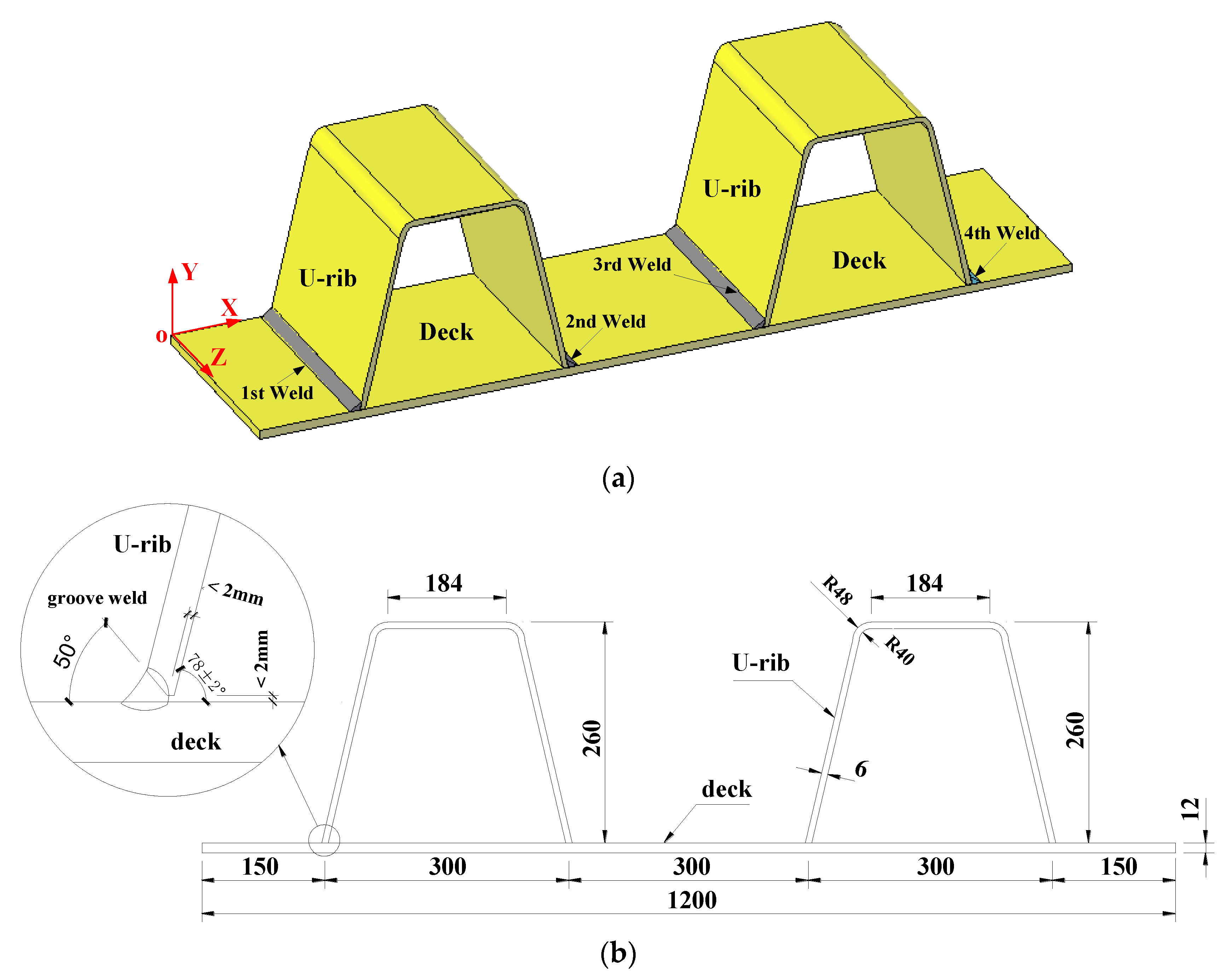
• The local fine model (LFM) of DRWDs is established with Jiangyin Yangtze River Highway Bridge as the engineering background. The eight-node solid element provided by ANSYS is used to perform a FEM simulation on the top decks, ribs, and weld structure in 1.5 U ribs. During the modeling process, the Solid70 elements and Solid185 elements are adopted for heat transfer analysis and mechanical analysis, respectively. The welding seam details are shown in Figure 1. The length of local fine model is 900 mm and the width is 300 mm.
• The multi-scale model of entire OSDs is modeled by embedding the LFM into the GM as shown in Figure 10a. In this model, the shell elements and solid elements are rigidly connected and the multipoint constraint algorithm is used in contact calculation. In contact connection area, the target element (Targe170) and contact element (Conta175) are defined as solid element (Solid185) surface and shell element (Shell63) nodes, respectively. All translational degrees of freedom (DOFs) are constrained at both ends of the multi-scale model of entire OSDs.
• The thermal structure coupling method is adopted to simulate the temperature field and stress field of welding process in the multi-scale model of entire OSDs. This process is the same as that in Section 2.2, so will not be repeated here. Then, the external fatigue loading is applied to the deck surface of the multi-scale model to obtain the true coupled stress time history of DRWDs. The blue distributed loads in Figure 10b are the external cyclic loads, which are applied on top of the welded joint in a 50 mm × 300 mm area, to simulate the effect of cyclic loading on the residual stress relaxation.

4. Residual Stress Relaxation of DRWDs by External Cyclic Loading

4.1. Welding Residual Stress Release of DRWDs under Constant Amplitude Cyclic Loading

To investigate the combination influence of stress ratio and stress amplitude on the multi-axial residual stress relaxation effect of DRWDs, 25 constant amplitude cyclic loading cases are applied to the multi-scale coupled stress analysis model of OSDs. The five transverse stress amplitudes from 10 MPa to 130 MPa are designed, and five stress ratios from ‒0.5 to 0.5 with 0.25 increments for each of five stress amplitudes are studied. For convenience, the transverse stress amplitude, longitudinal stress amplitude, and stress ratio are denoted as TSA, LSA, and R. The nominal stress is usually used to calculate the fatigue life in the specifications. As a result, the transverse stress is used in this paper to set loading cases and the location of the transverse stress is 1.5 t away from the weld toe, where t = plate thickness. That is to say, the TSA (the stress is perpendicular to the welding direction) and LSA (the stress is parallel to the welding direction) at the joints 1.5 t away from the weld toe (Figure 11) are extracted as TSA and LSA, respectively, after the external load is applied to the multi-scale coupled stress analysis model of OSDs.

A residual stress relaxation coefficient A is introduced to represent the change of welding residual stress relaxation under different loading cycles, which can be expressed as follows:

$$\mathrm{A}={\left({\sigma }_{res}\right)}_{after}/{\left({\sigma }_{res}\right)}_{ini},$$

(7)

where ${\left({\sigma }_{res}\right)}_{after}$ is the stable coupling stress that considers the welding residual stress and the mechanical stress induced by external cyclic loading; ${\left({\sigma }_{res}\right)}_{ini}$ is the initial residual stress.

4.1.1. Number of External Loading Cycles

Because of symmetry, the middle half of the deck-rib component in LFM is taken for investigating. The X axis and Z axis in Figure 12, Figure 13, Figure 14 and Figure 15 are correspond to the local coordinate in Figure 10b. Figure 12 depicts the distribution of ${\sigma }_x$ and ${\sigma }_z$ at Z = 150 mm along the X-axis (perpendicular to the weld seam) under external loading cycles from 0 to 10 for TSA = 130 MPa and R = 0.5. Figure 13 shows the distribution of ${\sigma }_x$ and ${\sigma }_z$ at X = 150 mm along the Z-axis (parallel to the weld seam). As the number of external loading cycles increased from 1 to 10, the distribution trend of welding residual stress remained almost unchanged, and the stress decreased until it was stable. Most of the welding residual stress release (about 95%) occurred in the first loading cycle. Therefore, the stable welding residual stress after 10 loading cycles was used to investigate the effect of stress amplitude and stress ratio on residual stress relaxation. As shown in Figure 13, the stress at two ends decreased gradually until extinction due to the constraint conditions, but was uniform at Z = 50‒250 mm.

4.1.2. Stress Amplitude of External Cyclic Loading

To study the influence of stress amplitude on residual stress relaxation, the TSA is increased from 10 MPa to 130 MPa. Figure 14 and Figure 15 show the distribution of residual stress along the X-axis (perpendicular to the weld seam) and Z-axis (parallel to the weld seam), respectively, under TSA from 0 MPa to 130 MPa for R = 0.5. As the TSA increases from 10 MPa to 130 MPa, the peak values of ${\sigma }_x$ and ${\sigma }_z$ gradually decrease, the magnitude of stress relaxation increase, and the overall distribution characteristics of the residual stress remain unchanged.

Figure 16 and Figure 17 show that the welding residual stress relaxation coefficient A varies with the longitudinal and transverse stress amplitude as R increases from ‒0.5 to 0.5. First, it is observed that A decreases gradually with the increase in the loading stress amplitude, which indicates that the stress release increases gradually. The value of A remains 1 for TSA = 10MPa, which indicates that the residual stress is not relaxed in such cases. Second, the value of A decreases rapidly in the first loading cycle and then gradually becomes stable as the number of loading cycles increases from 0 to 10. Third, the final value of A depends on the stress amplitude and stress ratio. For example, the value of A is stable at about 0.92 for TSA = 100 MPa and R = 0.5.

To explain the conditions of residual stress relaxation,

Table 2. Transverse, longitudinal, and Mises stresses under different stress amplitudes for R = 0.5 (unit: MPa).

No.	${\left({\mathit{\sigma }}_{\mathit{r}\mathit{e}\mathit{s}}\right)}_{\mathit{i}\mathit{n}\mathit{i}}$			${\mathit{\sigma }}_{\mathit{a}\mathit{p}\mathit{p}}$			$\mathbf{B}=\frac{{\left({\mathit{\sigma }}_{\mathit{r}\mathit{e}\mathit{s}}\right)}_{\mathit{i}\mathit{n}\mathit{i}}\mathbf{+}{\mathit{\sigma }}_{\mathit{a}\mathit{p}\mathit{p}}}{{\mathit{f}}_{\mathit{y}}}$			A
	${\mathit{\sigma }}_{\mathit{x}}$	${\mathit{\sigma }}_{\mathit{z}}$	Mises 1	TSA	LSA	Mises	Tran.2	Long.3	Mises	Tran.	Long.	Mises
1	146.54	373.35	325.81	10.00	14.08	12.55	0.45	1.12	0.97	0.99	0.99	0.99
2				40.00	56.33	50.20	0.58	1.25	1.10	0.97	0.96	0.96
3				70.00	98.59	87.86	0.72	1.38	1.20	0.95	0.92	0.91
4				100.00	140.84	125.51	0.86	1.51	1.32	0.92	0.86	0.85
5				130.00	183.09	163.15	1.00	1.65	1.45	0.87	0.77	0.75

¹ Mises denotes the initial residual mises stress; ² Tran. denotes the transverse stress of B, which is expressed as $\mathrm{B}=({\sigma }_x+TSA)/f_y$; ³ Long. denotes the longitudinal stress of B, which is expressed as $\mathrm{B}=({\sigma }_z+LSA)/f_y$.

shows the relationships among the residual stress relaxation coefficient A, the initial residual stress (${\left({\sigma }_{res}\right)}_{ini}$), the structure stress induced by the external loading (${\sigma }_{app}$), and the yield strength of material ($f_y$) as TSA increases from 10 MPa to 130 MPa for R = 0.5. As illustrated in Table 2, the value of A = 0.99 for TSA = 10.00 MPa and LSA = 14.08 MPa. This shows that the residual stress hardly relaxes and the transverse stress is B < 1; the longitudinal stress is B > 1 and the Mises stress is B < 1 in such cases. For the other four cases in Table 1, no matter how the longitudinal and transverse stress of B changes, the Mises stress of B and the value of A are always less than 1, which reveals that stress relaxation occurs. Therefore, whether the stress relaxation occurs under the mechanical stress, which is induced by the external cyclic loading, depends on the sum of initial residual stress (${\left({\sigma }_{res}\right)}_{ini}$); and structure stress (${\sigma }_{app}$) exceeds the yield strength of the material ($f_y$), rather than observing the stress variation of a certain uniaxial.

4.1.3. Stress Ratio of External Cyclic Loading

Figure 18 shows that the transverse/longitude stress relaxation coefficient A is related to transverse/longitude stress amplitudes and stress ratios. Taking Figure 18a as example, the welding residual stress relaxation coefficient A decreases with the increase of the stress amplitude (TSA), and decreases approximately linearly with the stress ratio (R). This is because the superposition of external cyclic stress and welding residual stress produces plasticity in a larger area, which leads to greater relaxation of welding residual stress.

4.1.4. Release Formula of Welding Residual Stress under the Constant Amplitude Cyclic Loading

According to the numerical simulation results, a release formula of welding residual stress relaxation coefficient A based on the stress amplitude, stress ratio, and material yield stress of external load was proposed:

$$\{\begin{array}{cc}A=1\hfill & \frac{{\left({\sigma }_{res}\right)}_{ini}+{\left({\sigma }_{app}\right)}_{mises}}{f_y}\le 1\hfill \\ A=\left(p_1+p_2\cdot \mathrm{R}\right)\cdot {\left(\frac{{\sigma }_{app}}{f_y}\right)}^2+p_3\hfill & \frac{{\left({\sigma }_{res}\right)}_{ini}+{\left({\sigma }_{app}\right)}_{mises}}{f_y}>1,\hfill \end{array}$$

(8)

where A is the welding residual stress relaxation coefficient; R is the stress ratio; ${\left({\sigma }_{res}\right)}_{after}$ is the stable coupling stress that considers the welding residual stress and the mechanical stress induced by external cyclic loading; ${\left({\sigma }_{res}\right)}_{ini}$ is the initial residual stress; ${\sigma }_{app}$ is the mechanical stress induced by external cyclic loading; mises is the Mises mechanical stress induced by external cyclic loading; $f_y$ is the yield strength of the material, which is 345 MPa for Q345 steel; and P1, P2, and P3 are coefficients with values of ‒0.6482, ‒0.2573, and 0.9875, respectively.

Figure 19 compares the FE simulation results with the predicted value in Equation (8). By regression analysis, the fitting results are within the confidence level of 99%. Since Equation (8) has regularized the yield stress of the material, it is also applicable to the residual stress relaxation of different steels.

4.2. Welding Residual Stress Release of DRWDs under Variable Amplitude Cyclic Loading

During the service period of the bridge, the steel deck bears the repeated action of the vehicle loading directly, and the wheel loading is usually the variable amplitude loading. For the sake of convenience, 12 variable-amplitude loading cases are designated, as shown in

Table 3. Twelve variable-amplitude cyclic loading cases (unit: MPa).

Cases	${({\mathit{\sigma }}_{\mathit{a}\mathit{p}\mathit{p}})}_{\mathbf{1}}$	${({\mathit{\sigma }}_{\mathit{a}\mathit{p}\mathit{p}})}_{\mathbf{2}}$	${({\mathit{\sigma }}_{\mathit{a}\mathit{p}\mathit{p}})}_{\mathbf{3}}$	${({\mathit{\sigma }}_{\mathit{a}\mathit{p}\mathit{p}})}_{\mathbf{4}}$	${({\mathit{\sigma }}_{\mathit{a}\mathit{p}\mathit{p}})}_{\mathbf{5}}$
C1	130	40	40	40	40
C2	40	130	40	40	40
C3	40	40	130	40	40
C4	40	40	40	130	40
C5	40	40	40	40	130
C6	32.5	65	65	65	65
C7	65	65	65	65	65
C8	97.5	65	65	65	65
C9	130	65	65	65	65
C10	130	100	65	65	65
C11	130	65	100	65	65
C12	65	130	100	65	65

, and their influence on the residual stress release in DRWs is analyzed. The symbols ${({\sigma }_{app})}_n\left(n=1,2,\dots 5\right)$ denote the stress of the nth cyclic loading. According to the study of 25 constant amplitude loading cases in the previous section, the residual stress relaxation mostly occurred in the first loading cycle, and tended to be stable after five cycles. Therefore, the number of cycles in this section is set to five. Taking C1 and C12 as examples, the stress time‒history curves are shown in Figure 20.

For convenience, the initial transverse residual stress (transverse residual stress at n = 0) is denoted as ${\left({\sigma }_x\right)}_{ini}$; the initial longitudinal residual stress is denoted as ${\left({\sigma }_z\right)}_{ini}$. According to the simulation results in Section 2.3, ${\left({\sigma }_x\right)}_{ini}$ was 146.54 MPa, and ${\left({\sigma }_x\right)}_{ini}$ was calculated to be 147.32 MPa based on the extracted FE data.

In C1‒C5, the cyclic order of the maximum loading is 1 to 5, respectively, and their common feature is that they have the same maximum loading (130 MPa). As shown in Figure 21a, the final ${\sigma }_x$ at n = 5 are the same in C1‒C5, which indicates that the residual stress releases in those five cases is the same. The reason is that the maximum value of the variable amplitude cyclic loading they are subjected to is equal. Moreover, the residual stress release only occurs in the first cycle in C1. However, residual stress release occurred in the first and second cycles, the first and third cycles, the first and fourth cycles, and the first and fifth cycles in C2‒C5, respectively. This is due to the fact that the magnitude of residual stress relaxation is controlled by the maximum stress in the variable amplitude cyclic loading. Finally, the stress will not continue to be released if the DRWDs have the same or smaller amplitude loading, after the residual stress is released. For instance, if the maximum stress of cyclic loading appears in the first cycle, then thereafter the loading stress will be smaller than that of the first cycle in C1. The corresponding residual stress release only appears in the first cycle, and there is almost no relaxation of residual stress in the second to fifth stress loading processes. In C3, although the absolute maximum stress appears in the third cycle, the relative maximum stress is ${({\sigma }_{app})}_1$ in the first cycle, and the first stress relaxation occurs in this cycle. In the second cycle,${({\sigma }_{app})}_2={({\sigma }_{app})}_1$, the residual stress of the cycle has little relaxation. In the third cycle, ${({\sigma }_{app})}_3>{({\sigma }_{app})}_1={({\sigma }_{app})}_2$, the residual stress of the cycle is released a second time. After that ${({\sigma }_{app})}_3>{({\sigma }_{app})}_1={({\sigma }_{app})}_2={({\sigma }_{app})}_4={({\sigma }_{app})}_5$, there is little relaxation of residual stress in the fourth and fifth cycles.

As depicted in Table 3, the second to fifth cyclic loading stresses were all 65 MPa, but the first cyclic loading stresses increased from 31.5 MPa to 130 MPa in C6‒C9. Figure 21b shows the stable transverse residual stress after relaxation at the weld toe in C6‒C9. It is seen that stress release only occurs during the first cyclic loading, except for C6. This is because the first cyclic stress (${({\sigma }_{app})}_1$) in C7‒C9 has reached the maximum stress amplitude. In C6, stress relaxation occurs under the first loading cycle. During the second loading cycle, the stress continues to relax, because the second cyclic stress is greater than the first cyclic stress (${({\sigma }_{app})}_2 > {({\sigma }_{app})}_1$). At this point, the slope of the stress decline line is greater than that of the first stress relaxation, indicating that the stress relaxation decreases nonlinearly with the increase in loading stress. In C9‒C12, three stress amplitudes were set to 65 MPa, 100 MPa, and 130 MPa, respectively. The first cyclic loading stress of C9‒C11 reached the maximum. As shown in Figure 21c, the total stress release in the four cases is almost equal after five cycles. In C9‒C11, the stress release only occurred during the first cyclic loading, while stress was released in the first two cyclic loadings of C12.

Table 4. The transverse residual stress and release stress under variable-amplitude cyclic loading cases (unit: MPa).

Cases	The Transverse Residual Stress (TRS) and Release Stress (RS)
	n = 1		n = 2		n = 3		n = 4		n = 5
	TRS	RS	TRS	RS	TRS	RS	TRS	RS	TRS	RS
C1	131.99	14.78	131.89	0.15	131.89	0.00	131.89	0.00	131.89	0.00
C2	143.59	3.03	131.99	11.75	131.90	0.10	131.90	0.00	131.90	0.00
C3	143.59	3.03	143.43	0.09	131.99	11.66	131.89	0.02	131.89	0.00
C4	143.59	3.03	143.43	0.09	143.43	0.00	131.87	11.54	131.82	0.12
C5	143.59	3.03	143.43	0.09	143.43	0.00	143.43	0.00	132.09	11.79
C6	144.00	2.69	141.60	2.41	141.50	0.09	141.50	0.00	141.50	0.00
C7	141.60	5.02	141.34	0.21	141.34	0.00	141.34	0.00	141.34	0.00
C8	137.59	9.12	137.49	0.12	137.49	0.00	137.49	0.00	137.49	0.00
C9	131.99	14.78	131.88	0.17	131.88	0.00	131.88	0.00	131.88	0.00
C10	131.99	14.78	131.84	0.19	131.84	0.00	131.84	0.00	131.84	0.00
C11	131.99	14.78	131.86	0.15	131.86	0.00	131.86	0.00	131.86	0.00
C12	141.60	5.02	131.99	9.76	131.85	0.20	131.85	0.00	131.85	0.00

shows the transverse residual stress and release stress under variable-amplitude loading cycles from 0 to 5. For variable amplitude loading cases, if ${({\sigma }_{app})}_1 \ge {({\sigma }_{app})}_2 \ge {({\sigma }_{app})}_3 \ge {({\sigma }_{app})}_4 \ge {({\sigma }_{app})}_5$, the residual stress is released only during the first stress cycle. Therefore, the residual stress release behavior is controlled by the maximum amplitude stress. Once the residual stress is released, the stress will not continue to be released if the DRWDs have the same or smaller amplitude loading.

As illustrated in

Table 5. Comparison of simulation (Si) and calculation (Ca) values of transverse residual stress under variable-amplitude cyclic loading cases (unit: MPa).

Cases	The Transverse Residual Stress (TRS)
	n = 1		n = 2		n = 3		n = 4		n = 5
	Ca	Si	Ca	Si	Ca	Si	Ca	Si	Ca	Si
C1	131.99	132.54	131.89	132.39	131.89	132.39	131.89	132.39	131.89	132.39
C2	143.59	144.29	131.99	132.54	131.90	132.44	131.90	132.44	131.90	132.44
C3	143.59	144.29	143.43	144.19	131.99	132.54	131.89	132.52	131.89	132.52
C4	143.59	144.29	143.43	144.19	143.43	144.19	131.87	132.65	131.82	132.53
C5	143.59	144.29	143.43	144.19	143.43	144.19	143.43	144.19	132.09	132.40
C6	144.00	144.63	141.60	142.22	141.50	142.13	141.50	142.13	141.50	142.13
C7	141.60	142.30	141.34	142.09	141.34	142.09	141.34	142.09	141.34	142.09
C8	137.59	138.20	137.49	138.08	137.49	138.08	137.49	138.08	137.49	138.08
C9	131.99	132.54	131.88	132.36	131.88	132.36	131.88	132.36	131.88	132.36
C10	131.99	132.54	131.84	132.35	131.84	132.35	131.84	132.35	131.84	132.35
C11	131.99	132.54	131.86	132.38	131.86	132.38	131.86	132.38	131.86	132.38
C12	141.60	142.30	131.99	132.54	131.85	132.34	131.85	132.34	131.85	132.34

, the simulation and calculation values of ${\sigma }_x$ under variable-amplitude cyclic loading cases are compared. To simplify the calculation, it is assumed that the first stress releasing amount under constant amplitude cyclic loading is 95% of the total releasing amount under this stress amplitude, and the second release ratio is 100%, according to the release rule summarized in Section 4.1 of this paper. It can be seen from Table 4 that the residual stress under cyclic loading calculated by Equation (8) shows good agreement with the FE simulation results. The results of this paper can be used in actual bridge analysis to predict the real stress of DRWDs, considering the welding residual stress relaxation under vehicle loading. Therefore, the fatigue life of such type of welding details in OSDs during service can be accurately assessed.

5. Conclusions

Based on the above investigations, the main conclusions are as follows:

• The stress relaxation condition of weld residual stress under the mechanical stress, which is induced by the external cyclic loading, depends on the sum of initial residual stress (${\left({\sigma }_{res}\right)}_{ini}$) and Mises structure stress (${\left({\sigma }_{app}\right)}_{Mises}$) and exceeds the yield strength of the material ($f_y$), rather than observing the stress variation of a certain uniaxial (longitudinal or transverse stress).
• Most of the welding residual stress release (about 95%) occurred in the first loading cycle under the constant amplitude cyclic loading. As the number of external loading cycles increased, the overall distribution trend of welding residual stress remained almost unchanged, and the stress decreased until it was stable after five cycles.
• The welding residual stress relaxation coefficient A decreases with the increase in stress amplitude (TSA), and decreases approximately linearly with the stress ratio (R); that is to say, the releasing amount of welding residual stress increases with the increase in stress amplitude (TSA) and increases approximately linearly with the increase in the stress ratio (R).
• The release behavior of residual stress is controlled by the maximum amplitude stress in the variable amplitude cyclic loading. Thus, the stress will not continue to be released if the DRWDs have the same or smaller amplitude loading after the residual stress is released.

References

1. Hu, N.; Dai, G.L.; Yan, B. Recent development of design and construction of medium and long span high-speed railway bridges in China. Eng. Struct. 2014, 74, 233–241. [Google Scholar] [CrossRef]
2. Song, Y.S.; Ding, Y.L.; Wang, G.X. Fatigue-life evaluation of a high-speed railway bridge with an orthotropic steel deck integrating multiple factors. Perform. J. Constr. Facil. 2016, 30, 04016036. [Google Scholar] [CrossRef]
3. Ji, B.H.; Liu, R.; Chen, C. Evaluation on root-deck fatigue of orthotropic steel bridge deck. Constr. J. Steel. Res. 2013, 90, 174–183. [Google Scholar] [CrossRef]
4. Gaul, R. A Long Life Pavement for Orthotropic Bridge Decks in China. Geotech. Spec. Publ. 2015, 196, 1–8. [Google Scholar]
5. Ya, S.; Yamada, K. Fatigue evaluation of rib-to-deck welded joints of orthotropic steel bridge deck. J. Bridge Eng. 2015, 492–499. [Google Scholar] [CrossRef]
6. Guo, T.; Frangopol, D.M.; Chen, Y.W. Fatigue reliability assessment of steel bridge details integrating weigh-in-motion data and probabilistic finite element analysis. Comp. Struct. 2012, 112–113, 245–257. [Google Scholar] [CrossRef]
7. Liu, R.; Ji, B.; Wang, M.; Chen, C. Numerical evaluation of toe-deck fatigue in orthotropic steel bridge deck. Perform. J. Constr. Facil. 2015, 29, 04014180. [Google Scholar] [CrossRef]
8. Xiao, Z.G.; Yamada, K. Stress analyses and fatigue evaluation of rib-to-deck joints in steel orthotropic decks. Int. J. Fatigue 2008, 30, 1387–1397. [Google Scholar] [CrossRef]
9. Cheng, X.; Fisher, J.W.; Prask, H.J.; Gnäupel-Herold, T.; Yen, B.T.; Roy, S. Residual stress modification by post-weld treatment and its beneficial effect on fatigue strength of welded structures. Int. J. Fatigue 2003, 25, 1259–1269. [Google Scholar] [CrossRef]
10. Cui, C.; Bu, Y.Z.; Bao, Y. Strain energy-based fatigue life evaluation of deck-to-rib welded joints in osd considering combined effects of stochastic traffic load and welded residual stress. J. Bridge Eng. 2017, 23, 04017127. [Google Scholar] [CrossRef]
11. Xie, X.F.; Jiang, W.; Luo, Y.; Xu, S.; Gong, J.M.; Tu, S.T. A model to predict the relaxation of weld residual stress by cyclic load: Experimental and finite element modeling. Int. J. Fatigue 2017, 95, 293–301. [Google Scholar] [CrossRef]
12. Farajian, M.; Nitschke, T.P.; Dilger, K. Mechanisms of residual stress relaxation and redistribution in welded high-strength steel specimens under mechanical loading. Weld. World 2010, 54, R366–R374. [Google Scholar] [CrossRef]
13. Han, S.; Lee, T.; Shin, B. Residual stress relaxation of welded steel components under cyclic load. Steel Res. 2002, 73, 414–420. [Google Scholar] [CrossRef]
14. Dattoma, V.; Giorgi, M.; Nobile, R. Numerical evaluation of residual stress relaxation by cycle load. J. Strain Anal. Eng. 2004, 39, 663–672. [Google Scholar] [CrossRef]
15. Wang, Q.; Liu, X.S.; Yan, Z.J. On the mechanism of residual stresses relaxation in welded joints under cyclic loading. Int. J. Fatigue 2017, 105, 43–59. [Google Scholar] [CrossRef]
16. Zhang, Q.H.; Cui, C.; Bu, Y.Z.; Liu, Y.M.; Ye, H.W. Fatigue tests and fatigue assessment approaches for rib-to-diaphragm in steel orthotropic decks. Constr. J. Steel Res. 2015, 114, 110–118. [Google Scholar] [CrossRef]
17. Cao, Y.B.; Ding, Y.L.; Song, Y.S.; Zhong, W. Fatigue Life Evaluation for Deck-Rib Welding Details of Orthotropic Steel Deck Integrating Mean Stress Effects. J. Bridge Eng. 2019, 24, 04018114. [Google Scholar] [CrossRef]
18. Cui, C.; Zhang, Q.; Bao, Y.; Han, S.; Bu, Y. Residual Stress Relaxation at Innovative Both-side Welded Rib-to-deck Joints under Cyclic Loading. Constr. J. Steel Res. 2019, 156, 9–17. [Google Scholar] [CrossRef]
19. Lee, C.H.; Chang, K.H.; Van Do, V.N. Finite element modeling of residual stress relaxation in steel butt welds under cyclic loading. Eng. Struct. 2015, 103, 63–71. [Google Scholar] [CrossRef]
20. Hensel, J.; Nitschke-Pagel, T.; Dilger, K. Residual stress-based fatigue design of welded structures. Mater. Perform. Character. 2018, 7, 630–642. [Google Scholar] [CrossRef]
21. Nelson, D.V.; McCrickerd, J.T. Residual-stress determination through combined use of holographic interferometry and blind-hole drilling. Exp. Mech. 1986, 26, 371–378. [Google Scholar] [CrossRef]
22. Schajer, G.S. Measurement of non-uniform residual stresses using the hole-drilling method. Part II—Practical application of the integral method. J. Eng. Mater. Technol. 1988, 110, 344–349. [Google Scholar] [CrossRef]
23. Teng, T.L.; Fung, C.P.; Chang, P.H.; Yang, C.W. Analysis of residual stresses and distortions in T-joint fillet welds. Int. J. Press. Vessels Pip. 2001, 78, 523–538. [Google Scholar] [CrossRef]
24. Wang, W.; Yan, S.; Kodur, V. Temperature induced creep in low-alloy structural Q345 steel. Mater. J. Civ. Eng. 2016, 28, 1–6. [Google Scholar] [CrossRef]
25. Yuan, G.; Shu, Q.; Huang, Z.; Li, Q. An experimental investigation of properties of Q345 steel pipe at elevated temperatures. Constr. J. Steel Res. 2016, 118, 41–48. [Google Scholar] [CrossRef] [Green Version]
26. Timoshenko, S.P.; Goodier, J.N. The Theory of Elasticity; McGraw-Hill: New York, NY, USA, 1951. [Google Scholar]
27. Chaboche, J.L. Time independent constitutive theories for cyclic plasticity. Int. Plast. J. 1986, 2, 149–188. [Google Scholar] [CrossRef]
28. Van Do, V.N.; Lee, C.H.; Chang, K.H. High cycle fatigue analysis in presence of residual stresses by using a continuum damage mechanics model. Int. J. Fatigue 2015, 70, 51–62. [Google Scholar]
29. Rousselier, G. On the plastic and viscoplastic constitutive equations-part I: Rules developed with internal variable concept. Press. J. Vessel. Technol. 1983, 105, 153–158. [Google Scholar]
30. Chaboche, J.L. On some modifications of kinematic hardening to improve the description of ratchetting effects. Int. Plast. J. 1991, 7, 661–678. [Google Scholar] [CrossRef]
31. Goldak, J.; Chakravarti, A.; Bibby, M. A new finite element model for welding heat sources. Metall. Trans. B 1984, 15, 299–305. [Google Scholar] [CrossRef]
32. Ucak, A.; Tsopelas, P. Accurate modeling of the cyclic response of structural components constructed of steel with yield plateau. Eng. Struct. 2012, 35, 272–280. [Google Scholar] [CrossRef]
33. Chaboche, J.L.; Lesne, P.M. A non-linear continuous fatigue damage model. Fatigue Fract. Eng. Mater. Struct. 1988, 11, 1–17. [Google Scholar] [CrossRef]
34. Tian, Q.; Zhuge, H.; Xie, X. Prediction of the Ultra-Low-Cycle Fatigue Damage of Q345qC Steel and its Weld Joint. Materials 2019, 12, 4014. [Google Scholar] [CrossRef] [PubMed] [Green Version]
35. Wang, J.B. Improvement of the Hysteretic Constitutive Model for Bridge Structural Steels and Its Application. Ph.D. Thesis, Zhejiang University, Hangzhou, China, 2016. (In Chinese). [Google Scholar]
36. Yu, Y.; Wang, X.; Chen, Z. Evaluation on steel cyclic response to strength reducing heat treatment for seismic design application. Constr. Build. Mater. 2017, 140, 468–484. [Google Scholar] [CrossRef]
Figure 1. Orthotropic steel deck (OSD) experimental specimens: (a) space diagram and measurement paths; (b) cross section and dimensions (units: mm).
Applsci 11 00253 g001
Figure 2. Experimental device: (a) test drilling equipment; (b) electric pole; (c) strain gauge.
Applsci 11 00253 g002
Figure 3. Diagram of the measurement paths: (a) cross section diagram; (b) plan diagram (units: mm).
Applsci 11 00253 g003
Figure 4. Diagram of the measurement points of layout paths: (a) cross section diagram; (b) plan diagram (units: mm).
Applsci 11 00253 g004
Figure 5. Hole-drilling locations of various paths: (a) P1, P4 and P5; (b) P2, P3, and P6.
Applsci 11 00253 g005
Figure 6. Finite element model (FEM) of the welded joints in the OSD: (a) displacement boundary; (b) mesh of FEM model.
Applsci 11 00253 g006
Figure 7. Temperature distribution in the thermal field (unit: degrees Celsius): (a) t = 30 s; (b) t = 150 s; (c) t = 360 s; (d) t = 1020 s; (e) the shape of welding molten pool at t = 1020 s; (f) t = 3420 s.
Applsci 11 00253 g007
Figure 8. Distribution of σ x and σ z on Paths P1 and P2: (a) σ x ; (b) σ z .
Applsci 11 00253 g008
Figure 9. Distribution of σ x and σ z on Paths P3 and P4: (a) σ x ; (b) σ z .
Applsci 11 00253 g009
Figure 10. A multi-scale coupled stress analysis model: (a) build model; (b) load model (unit: mm).
Applsci 11 00253 g010aApplsci 11 00253 g010b
Figure 11. Direction and location of the external cyclic loading (transverse stress amplitude (TSA) and longitudinal stress amplitude (LSA)).
Applsci 11 00253 g011
Figure 12. Distribution of residual stress along X-axis under external loading cycles from 0 to 10: (a) σ x ; (b) σ z .
Applsci 11 00253 g012
Figure 13. Distribution of residual stress along Z-axis under external loading cycles from 0 to 10: (a) σ x ; (b) σ z .
Applsci 11 00253 g013
Figure 14. Distribution of residual stress along X-axis under TSA from 0 MPa to 130 MPa: (a) σ x ; (b) σ z .
Applsci 11 00253 g014
Figure 15. Distribution of residual stress along Z-axis under TSA from 0 MPa to 130 MPa: (a) σ x ; (b) σ z .
Applsci 11 00253 g015
Figure 16. The variation curve of residual stress relaxation coefficient A with TSA: (a) R = ‒0.5; (b) R = ‒0.25; (c) R = 0; (d) R = 0.25; (e) R = 0.5.
Applsci 11 00253 g016aApplsci 11 00253 g016b
Figure 17. The variation curve of residual stress relaxation coefficient A with LSA: (a) R = ‒0.5; (b) R = ‒0.25; (c) R = 0; (d) R = 0.25; (e) R = 0.5.
Applsci 11 00253 g017aApplsci 11 00253 g017b
Figure 18. Relationship between stress relaxation coefficient A and stress amplitude and stress ratio: (a) σ x ; (b) σ z .
Applsci 11 00253 g018
Figure 19. Comparison between numerical simulation and formula prediction.
Applsci 11 00253 g019
Figure 20. The stress time‒history curves of C1 and C12: (a) C1; (b) C12.
Applsci 11 00253 g020
Figure 21. The transverse welding residual stress of C1‒C12: (a) C1‒C5; (b) C6‒C9; (c) C9‒C12.
Applsci 11 00253 g021