Robust Control of Electric Tail Reduction System: Uncertainty and Performance Index

Abstract

The electric tail reduction system of the unmanned helicopter contains uncertainty. To solve this problem, a constraint-following approach was applied to design a novel robust control for uncertain mechanical systems. The dynamic model of the uncertain electric tail reduction system was established by combining the load of the electric tail rotor and the flight state of the helicopter. Based on the Udwadia–Kalaba theory, a robust constraint following the control method was proposed to deal with the uncertainty of the system. In addition, to balance the steady-state performance and control cost of the system, a control parameter optimization design method was proposed to minimize the performance index. Furthermore, the unique solution of the optimal parameter can be obtained. Compared with the LQR control method, the effectiveness of the optimization method of robust constraint following control was verified.

1. Introduction

In recent years, the application of unmanned aircraft systems (UAS) in the military and civil fields is attracting people’s attention and interest [1]. Compared with fixed-wing unmanned aerial vehicles (UAVs), the rotor UAV has the characteristics of vertical take-off and landing, hovering, and flight at very low altitude, so it is used in a wider spectrum of applications [2]. With the rapid development of battery and motor technology, the advantages of unmanned electric helicopter have gradually been reflected [3]. On one hand, compared with the traditional fuel helicopter, the electric unmanned helicopter has the characteristics of lower noise, smaller vibration, higher reliability, and no pollution. On the other hand, the main flight performance algorithms and the design of autonomous flight control systems provide references for the development of electric helicopters. Therefore, unmanned electric helicopters with good mobility and low cost have recently been applied in various fields [4,5].

Unmanned electric helicopters have significant dynamic coupling, which is an inherently unstable and highly nonlinear underactuated system. These factors lead to serious challenges in dealing with robustness, disturbance rejection, decoupling, and other control problems [5]. In the control of an unmanned helicopter, some scholars have undertaken relevant research such as robust control [6,7], adaptive control [8,9,10,11], nonlinear attitude control [12], finite-time control [13], fuzzy control [14,15], and heading control of a composite helicopter [16].

Similar to the trend of aircraft electrification known as the “More Electric Aircraft” (MEA) approach, helicopter propulsion system and its flight control devices are undergoing a system optimization using electric actuators [3]. The electric tail reduction system of the unmanned helicopter is a typical electric actuator integrated system composed of a permanent magnet synchronous motor, reducer, and tail rotor, which is based on the background of independent speed control of the main rotor and the tail rotor. The speed of the tail rotor is variable, which could reduce the flight resistance of tail rotor when the helicopter flies forward, and improve the operational flexibility and efficiency reliability of the helicopter. In this way, the stagnation of the tail rotor when the main rotor speed suddenly drops can be avoided by decoupling the control of the main rotor and tail rotor. For these reasons, some scholars have undertaken related research. Han and Barakos studied variable tail rotor speed as a method to improve helicopter performance [17], and a dynamic response platform for collecting the thrust of an independent electric tail rotor was built by Zhang [3].

However, one of the main faults of a helicopter is the failure of the tail rotor, which occurs frequently and causes accidents [18]. The aerodynamic interference between the main rotor and the tail rotor will have a strong negative impact on the flight dynamics of conventional helicopters [19]. The electric tail reduction system is affected by uncertainty, aerodynamics, and dynamic coupling, which is determined by the inherent characteristics of the helicopter. Therefore, the research on its dynamic control is significant and challenging.

To control such nonlinear uncertain systems, many outstanding works have been done. A fuzzy backstepping sliding mode control for a manipulator with nonlinear disturbance observer was proposed by Truong [20]. A global fast sliding mode control to effectively compensate for the uncertain parameter variations and external disturbances was proposed by Iqbal [21]. The servo constraint control based on the Udwadia–Kalaba theory is one of the most advanced research directions at present. Udwadia proposed the tracking control of nonlinear mechanical systems based on the servo constraint control method [22,23,24,25]. In addition, he completed precise trajectory control with the advantage of less computation [26]. According to the Maggi Equation, Chen thought that the required constraint force could be satisfied by servo control [27]. Zhao researched dynamic modeling of multi-body systems using the Udwadia–Kalaba theory [28]. Sun applied the Udwadia–Kalaba theory to the tracking control of mobile robots and proposed a fuzzy method of an automotive electronic throttle system [29,30]. Furthermore, the Udwadia–Kalaba theory has been used by several researchers to deal with the tracking control and optimal design problems of mechanical systems [31,32,33,34].

The Udwadia–Kalaba theory considers the control problem by the second-order form constraints, which can be holonomic and nonholonomic [35]. In this paper, a constraint following control was proposed based on Udwadia–Kalaba theory regardless of the uncertainty in the electric tail reduction system. Then, an optimal design method that can balance system response and control cost was formulated.

The contributions of this paper are as follows. First, the dynamic model of the electric tail reduction system of unmanned helicopter was established, considering the flight state and main rotor condition of the unmanned helicopter. Second, based on the Udwadia–Kalaba theory, the constraint force was solved and the uncertainty was analyzed. Then, a robust constraint following control method was proposed to ensure the deterministic system performance: uniform boundedness and uniform ultimate boundedness. Finally, the performance index of the electric tail reduction system was established. A control parameter optimization design method was proposed, which minimizes the system performance index.

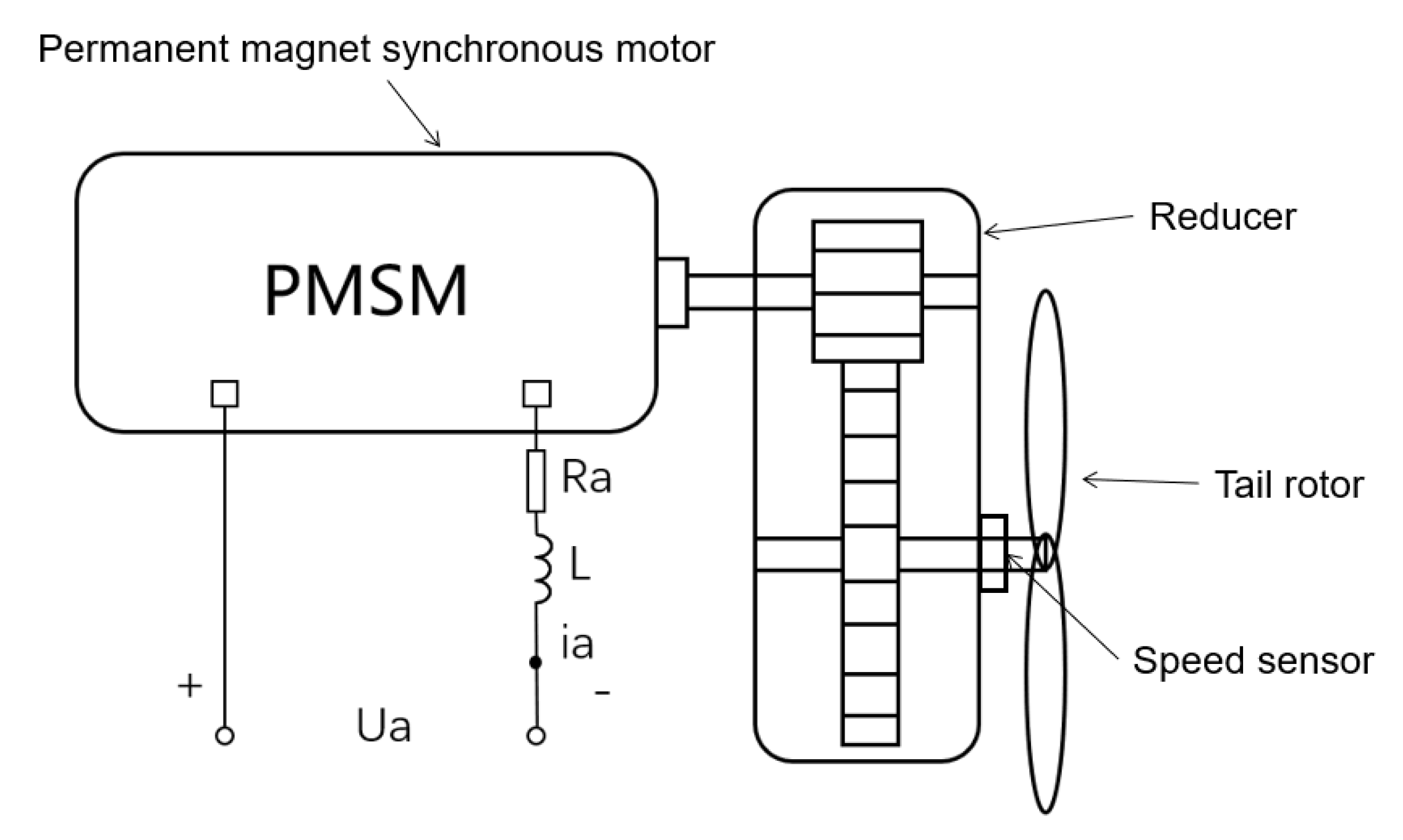
2. Dynamic Modeling of Electric Tail Reduction System

The electric tail reduction system of unmanned helicopter mainly includes the following parts: permanent magnet synchronous motor (PMSM), reducer, tail rotor, and speed sensor for measuring the tail rotor speed. The schematic diagram is shown in Figure 1. The input shaft of the reducer was directly connected with the outer rotor of the motor, and the output shaft was equipped with a tail rotor. The coupling was omitted and the number of components was reduced to achieve a compact structure, lightweight, and high power/weight ratio.

The dynamic model of the electric tail reduction system was established according to the following methods.

A PMSM uses permanent magnets embedded in the steel rotor to create a constant magnetic field. PMSMs are mainly controlled using direct torque control and field oriented control. Maxwell expounded the electromechanical system for the first time and established the dynamic equation using the Lagrange method [36]. The Lagrange–Maxwell Equation in three-phase stator reference frame is expressed as

$$\begin{array}{l}\frac{d}{dt}({\psi }_{abc})+{{\displaystyle R}}_S{{\displaystyle i}}_{abc}={{\displaystyle U}}_{abc}\\ J\ddot{\theta }+B\dot{\theta }+{{\displaystyle T}}_L={{\displaystyle i}}_{abc}^T\frac{\partial L_S}{\partial \theta }{{\displaystyle i}}_{abc}+{{\displaystyle i}}_{abc}^T\frac{\partial {\psi }_f}{\partial \theta }\end{array}$$

where ${\psi }_{abc}$ is the flux vector of three-phase stator shafting; ${{\displaystyle R}}_s$ is the resistance; ${{\displaystyle i}}_{abc}$ is the three-phase current vector of motor stator; ${{\displaystyle U}}_{abc}$ is the three-phase voltage vector of motor stator; $J$ is the rotational inertia of motor; $B$ is the viscous damping coefficient of motor; ${{\displaystyle T}}_L$ is the output torque; ${{\displaystyle L}}_s$ is the armature inductance; ${{\displaystyle \psi }}_f$ is the permanent magnet flux linkage; $\ddot{\theta }$ is the angular acceleration; and $\dot{\theta }$ and $\theta$ are the angular velocity and rotation angle of motor.

The current, voltage, and flux linkage in the above formula are transformed from three-phase stator shafting to two-phase rotor shafting at the same time, and the final electro-mechanical coupling dynamic equation of PMSM is

$$J\ddot{\theta }+B\dot{\theta }+{{\displaystyle T}}_L=\frac{3}{2}{{\displaystyle n}}_p[{{\displaystyle i}}_q{\psi }_f+({{\displaystyle L}}_d-{{\displaystyle L}}_q){{\displaystyle i}}_d{{\displaystyle i}}_q]$$

(1)

$${{\displaystyle T}}_e=\frac{3}{2}{{\displaystyle n}}_p[{{\displaystyle i}}_q{\psi }_f+({{\displaystyle L}}_d-{{\displaystyle L}}_q){{\displaystyle i}}_d{{\displaystyle i}}_q]$$

(2)

where ${{\displaystyle T}}_e$ is the electromagnetic torque; ${{\displaystyle T}}_L$ is the motor output torque; ${{\displaystyle L}}_d$, ${{\displaystyle L}}_q$ respectively is the motor AC-DC axis inductance; ${{\displaystyle n}}_p$ is the number of stator poles; ${{\displaystyle i}}_d$, ${{\displaystyle i}}_q$ respectively is the motor AC-DC axis current.

The above shows that the electromagnetic torque ${{\displaystyle T}}_e$ has three parts: (1) the torque $J\ddot{\theta }$ generated by rotor rotation, (2) the loss $B\dot{\theta }$ caused by the viscous damping of the motor, and (3) the output torque ${{\displaystyle T}}_L$ of the motor.

According to the selected reducer, the dynamic equation of the reducer is

$${{\displaystyle T}}_L=\frac{1}{\lambda \eta }{{\displaystyle T}}_r$$

(3)

with

$$\eta ={\eta }_1{\eta }_2$$

where ${{\displaystyle T}}_L$ is the motor output torque; ${{\displaystyle T}}_r$ is the reducer output torque; $\lambda$ is the reduction ratio; $\eta$ is the reducer transmission total efficiency; ${\eta }_1$ is the efficiency of the bearing; and ${\eta }_2$ is the efficiency of the gear transmission.

The tail rotor balances the counter torque of the main rotor by producing the yaw moment and carries out the heading operation. Then, the dynamic equation of the tail rotor is proposed by considering the time-varying load during the helicopter flight process. The dynamic equation of the tail rotor is obtained as

$${{\displaystyle T}}_r={{\displaystyle J}}_t\frac{1}{\lambda }\ddot{\theta }+{{\displaystyle T}}_t$$

(4)

By the reduction ratio between the tail rotor and the motor, we have

$${{\displaystyle \dot{\theta }}}_m=\frac{1}{\lambda }\dot{\theta }$$

(5)

$${{\displaystyle \ddot{\theta }}}_m=\frac{1}{\lambda }\ddot{\theta }$$

(6)

where ${{\displaystyle \dot{\theta }}}_m$ and ${{\displaystyle \ddot{\theta }}}_m$ are the angular velocity and acceleration of electric tail rotor of unmanned helicopter; ${{\displaystyle T}}_t$ is the tail rotor load; and ${{\displaystyle J}}_t$ is the rotational inertia of tail rotor.

The tail rotor load depends on the torque generated by the main rotor in the helicopter coordinate system and the yaw demand of the whole machine. Therefore, we considered the torque of the main rotor. The relationship between the tail rotor load and main rotor power is [3]

$${{\displaystyle T}}_t={{\displaystyle c\xi }}_{ynp}(\frac{{{\displaystyle P}}_M}{{{\displaystyle \omega }}_M}+{{\displaystyle M}}_f)$$

(7)

where ${{\displaystyle M}}_f$ is the yaw moment for helicopter; constant $c$ is the proportional factor of tail rotor thrust to tail rotor load; constant ${{\displaystyle \xi }}_{ynp}$ is the maneuver reserve factor; and ${{\displaystyle \omega }}_M$ is the main rotor speed.

The main rotor power ${{\displaystyle P}}_M$ of the helicopter consists of the following three parts by [37]

$${{\displaystyle P}}_M={{\displaystyle P}}_{pM}+{{\displaystyle P}}_{iM}+{{\displaystyle P}}_{paraM}$$

(8)

where ${{\displaystyle P}}_{pM}$ is the profile power; ${{\displaystyle P}}_{iM}$ is the induced power; and ${{\displaystyle P}}_{paraM}$ is the parasite power. The specific expressions of the above three types of power are as follows:

$$\begin{array}{l}{{\displaystyle P}}_{pM}=\frac{1}{2}{{\displaystyle \rho }}_M\pi {{\displaystyle R}}_M^2{{\displaystyle ({{\displaystyle R}}_M{{\displaystyle \omega }}_M)}}^3{{\displaystyle M}}_p\\ {{\displaystyle P}}_{iM}={{\displaystyle F}}_M{{\displaystyle V}}_{iM}\\ {{\displaystyle P}}_{paraM}=DV\end{array}$$

(9)

where ${{\displaystyle \rho }}_M$ is the air density; ${{\displaystyle R}}_M$ is the main rotor radius; $V$ is the helicopter horizontal forward flight speed. The specific expressions of profile power coefficient ${{\displaystyle M}}_p$, rotor pull force ${{\displaystyle F}}_M$, and parasite drag $D$ are shown as follows:

$$\begin{array}{c}{{\displaystyle M}}_p=\frac{1}{4}{{\displaystyle K}}_p{{\displaystyle C}}_{xp}\sigma [1+0.75(1+5{{\displaystyle \mu }}_m^2){{\displaystyle {{\displaystyle a}}_{1E}}}^2+4.7{{\displaystyle \mu }}_m^2]\hfill \\ {{\displaystyle F}}_M=\sqrt{{{\displaystyle G}}^2+{{\displaystyle D}}^2}\hfill \\ D=\frac{1}{2}{{\displaystyle \rho }}_M{{\displaystyle V}}^2{{\displaystyle C}}_{xf}{{\displaystyle S}}_f{{\displaystyle K}}_{df}\hfill \end{array}$$

(10)

where ${{\displaystyle K}}_p$ is the blade shape factor; ${{\displaystyle C}}_{xp}$ is the profile coefficient; $\sigma$ is the rotor solidity; ${{\displaystyle C}}_{xf}$ is the angle of attack resistance coefficient; ${{\displaystyle S}}_f$ is the fuselage top view area; ${{\displaystyle K}}_{df}$ is the parasite correction coefficient; ${{\displaystyle C}}_{xp}=0.009+0.0067({{\displaystyle \mu }}_m-0.3)$; and ${{\displaystyle a}}_{1E}=0.35{{\displaystyle \mu }}_m$.

The helicopter forward ratio is

$${{\displaystyle \mu }}_m=\frac{V}{{{\displaystyle R}}_M{{\displaystyle \omega }}_M}$$

(11)

The helicopter gravity is

$$G=mg$$

(12)

The induced power is the power consumed by the helicopter to exhaust the air downward and generate the pulling force. It is closely related to the forward flying speed of the helicopter, and is the main part of the power required by the main rotor when the helicopter hovers or flies forward at a small speed. The induced speed of helicopter hovering can be obtained as

$${{\displaystyle V}}_h=\sqrt{\frac{G}{2{{\displaystyle \rho }}_M\pi {{\displaystyle R}}_M^2}}$$

(13)

The induced speed of a helicopter at high-speed can be obtained as

$${{\displaystyle V}}_g=\frac{{{\displaystyle F}}_M}{2{{\displaystyle \rho }}_M\pi {{\displaystyle R}}_M^{2}V}$$

(14)

In general, the induced velocity of a helicopter is expressed as a piecewise function of hover induced velocity and high-speed induced velocity. However, when hovering mode and high-speed mode are switched, the induced speed estimated by the above method is easy to produce mutation. Therefore, the following weighted estimation method is applied to calculate the induced velocity of high-speed flight:

$${{\displaystyle V}}_{iM}={{\displaystyle V}}_h{{\displaystyle e}}^{(-\frac{KV}{{{\displaystyle V}}_h})}+{{\displaystyle V}}_g(1-{{\displaystyle e}}^{(-\frac{KV}{{{\displaystyle V}}_h})})$$

(15)

where $K$ is correction factor. Based on Equations (7)–(15), the tail rotor load can be solved.

In this paper, the surface mounted rotor structure based on symmetrical magnetic circuit was used (${{\displaystyle L}}_q={{\displaystyle L}}_d$). Therefore, by combining Equations (1)–(7), the dynamic equation of the electric tail reduction system is

$$\frac{3}{2}{{\displaystyle n}}_p{\psi }_f{{\displaystyle i}}_q={{\displaystyle J}}_{tr}{{\displaystyle \ddot{\theta }}}_m+{{\displaystyle B}}_{tr}{{\displaystyle \dot{\theta }}}_m+{{\displaystyle T}}_{tr}$$

where ${{\displaystyle J}}_{tr}$ is the equivalent rotational inertia; ${{\displaystyle B}}_{tr}$ is the equivalent viscous damping coefficient; and ${{\displaystyle T}}_{tr}$ is the equivalent load. The specific expressions are

$$\begin{array}{l}{{\displaystyle J}}_{tr}=J\lambda +\frac{1}{\lambda \eta }{{\displaystyle J}}_t\\ {{\displaystyle B}}_{tr}=B\lambda \\ {{\displaystyle T}}_{tr}=\frac{1}{\lambda \eta }{{\displaystyle T}}_t\end{array}$$

3. Robust Constraint Following Control

3.1. Uncertain Mechanical System

The dynamic equation of mechanical system with uncertainty can be obtained by the Udwadia–Kalaba theory [38]:

$$M(q(t),\sigma (t),t)\ddot{q}(t)=\tau (t)+Q(q(t),\dot{q}(t),\sigma (t),t)+Q^{\mathrm{c}}(q(t),\dot{q}(t),\sigma (t),t)$$

(16)

where $t\in R$ is the time independent variable; $q\in {{\displaystyle R}}^n$ is the coordinate (not necessarily the generalized coordinate and based on the specific problem); $\dot{q}\in {{\displaystyle R}}^n$ is the velocity; $\ddot{q}\in {{\displaystyle R}}^n$ is the acceleration; $\sigma \in {\displaystyle \sum \subset {{\displaystyle R}}^p}$ is the uncertainty parameter (possibly time-varying vector). In addition, $M(q,\sigma ,t)$ is the inertia matrix, $\tau \in {{\displaystyle R}}^n$ is the control input, $Q(q,\dot{q},\sigma ,t)$ is the force imposed on the system (centrifugal force, gravitational force are included here, but control input is not here), $Q^{\mathrm{c}}(q,\dot{q},\sigma ,t)$ is the constraint force. The functions $M(\cdot )$, $Q(\cdot )$, and ${{\displaystyle Q}}^c(\cdot )$ are assumed to be continuous.

The servo constraint is considered in the following form:

$${\displaystyle \sum _{i=1}^n{A}_{li}(q,t)}{\dot{q}}_i+A_l(q,t)=0{,}_{}^{}{{}_{}^{}}_{}^{}{{}_{}^{}}_{}^{}l=1,2,\cdots ,m$$

(17)

where $A_{li}(\cdot )$ and $A_l$ are both ${{\displaystyle C}}^1$, $1\le m\le n$.

The first order constraint (17) is mainly a limit of the velocity and displacement. The matrix form can be expressed as

$$A(q,t)\dot{q}=c(q,t)$$

(18)

where $c={{\displaystyle [{{\displaystyle c}}_1{{\displaystyle ,c}}_2,\cdots ,{{\displaystyle c}}_m]}}^T$, $A={{\displaystyle [A_{li}]}}_{m\times n}$.

By Equation (17), the second order form of the constraint equation is shown as follows:

$${\displaystyle \sum _{i=1}^n\frac{d}{dt}{A}_{li}}(q,t){\dot{q}}_i+{\displaystyle \sum _{i=1}^n{A}_{li}(q,t)}{\ddot{q}}_i+\frac{d}{dt}{A}_l(q,t)=0$$

(19)

where

$$\frac{d}{dt}{A}_{li}(q,t)={\displaystyle \sum _{k=1}^n\frac{\partial A_{li}(q,t)}{\partial {{\displaystyle q}}_k}}{{\displaystyle \dot{q}}}_k+\frac{\partial A_{li}(q,t)}{\partial t}$$

(20)

$$\frac{d}{dt}{A}_l(q,t)={\displaystyle \sum _{k=1}^n\frac{\partial A_l(q,t)}{\partial {{\displaystyle q}}_k}}{{\displaystyle \dot{q}}}_k+\frac{\partial A_l(q,t)}{\partial t}$$

(21)

Equation (19) can be obtained

$$\begin{array}{c}{\displaystyle \sum _{i=1}^n{A}_{li}}(q,t){\ddot{q}}_i=-{\displaystyle \sum _{i=1}^n\frac{d}{dt}{A}_{li}}(q,t)\dot{q}-\frac{d}{dt}{A}_l(q,t)\hfill \\ =:b_i(\dot{q},q,t)\hfill \end{array}{,}_{}^{}{{}_{}^{}}_{}^{}{{}_{}^{}}_{}^{}l=1,2,\cdots ,m$$

(22)

or

$$A(q,t)\ddot{q}=b(\dot{q},q,t)$$

(23)

where $b={{\displaystyle [{{\displaystyle b}}_1{{\displaystyle ,b}}_2,\cdots ,{{\displaystyle b}}_m]}}^T$ and $A={{\displaystyle [A_{li}]}}_{m\times n}$.

Remark 1.

Equations (17)–(23) were derived from [39]. In engineering applications, it is rational to constraint following approximately when initial conditions are uncertain and uncertainties exist. In other words, Equation (23) does not need to strictly follow performance requirements. Therefore, the servo constraint problem can be understood as: determine the servo control$\tau$so that the controlled system approximately approaches the constraint (18). If there is no uncertainty in the mechanical system (16), then$\sigma$ is known.

Assumption 1.

The inertia matrix$M(q,\sigma ,t)$is positive definite such as that for each${{\displaystyle (q,t)\in R}}^n\times R$,$\sigma \in \sum$.

Assumption 2.

The constraint (23) is consistent. That is, for given$A$and$b$, there exists at least one solution$\ddot{q}$. This assumption ensures$A{{\displaystyle A}}^{+}b=b$, which means the existence of the Moore–Penrose generalized inverse of$A$. On the contrary, if the constraint Equation (23) is inconsistent, then$\tau$is no solution in the servo constraint problem.

Theorem 1.

Considering the mechanical system (16) and the constraint (23), suppose that rank$A(q,t)\ge 1$for each$q$and$t$, according to Assumptions 1 and 2, the uncertain mechanical system’s constraint force conforms to Lagrange’s form of d’Alembert’s principle, which can be expressed as follows [24,40]:

$$\begin{array}{l}{{\displaystyle Q}}_S(q,\dot{q},\sigma ,t)=M^{1/2}(q,\sigma ,t){(A(q,t)M^{-1/2}(q,\sigma ,t))}^{+}\\ {{\displaystyle }}_{}^{}[b(q,\dot{q},t)-A(q,t)M^{-1}(q,\sigma ,t)(Q(q,\dot{q},\sigma ,t)+Q^c(q,\dot{q},\sigma ,t))]\end{array}$$

(24)

Equation (16) is rewritten as

$$Q(q(t),\dot{q}(t),\sigma (t),t)+Q^{\mathrm{c}}(q(t),\dot{q}(t),\sigma (t),t)=M(q(t),\sigma (t),t)\ddot{q}(t)-\tau (t)$$

Remark 2.

The detailed proof process of Theorem 1 can be found in [24]. Theorem 1 shows that an exact mathematical model is necessary for the constraint force. Udwadia verified that when the initial conditions are satisfied and the uncertainties are known, the control input$\tau ={{\displaystyle Q}}_S$can be used to drive the system to meet the constraint (23) [26]. However, in practical engineering applications, uncertainties exist and are unknown. For example, in the electric tail reduction system, there are uncertainties in model parameters and tail rotor load. Therefore, we will consider the design of the robust constraint following the control with uncertainties.

3.2. Robust Constraint Following Control Design

While designing the control $\tau$, we considered the uncertainties of each part of the electric tail reduction system including the uncertainty of the equivalent rotational inertia ${{\displaystyle J}}_{tr}$, the parameter uncertainty of the equivalent viscous damping coefficient ${{\displaystyle B}}_{tr}$ and the external disturbance dynamic uncertainty of the equivalent load ${{\displaystyle T}}_{tr}$. It is assumed that the matrix ${{\displaystyle J}}_{tr}$, ${{\displaystyle B}}_{tr}$, ${{\displaystyle T}}_{tr}$ can be decomposed into the following forms [38]:

$$\begin{array}{l}{{\displaystyle J}}_{tr}({{\displaystyle \theta }}_m,\sigma ,t)={{\displaystyle \overline{J}}}_{tr}({{\displaystyle \theta }}_m,t)+{{\displaystyle \Delta J}}_{tr}({{\displaystyle \theta }}_m,\sigma ,t)\\ {{\displaystyle B}}_{tr}({{\displaystyle \theta }}_m,{{\displaystyle \dot{\theta }}}_m,\sigma ,t)={{\displaystyle \overline{B}}}_{tr}({{\displaystyle \theta }}_m,{{\displaystyle \dot{\theta }}}_m,t)+{{\displaystyle \Delta B}}_{tr}({{\displaystyle \theta }}_m,{{\displaystyle \dot{\theta }}}_m,\sigma ,t)\\ {{\displaystyle T}}_{tr}({{\displaystyle \theta }}_m,{{\displaystyle \dot{\theta }}}_m,\sigma ,t)={{\displaystyle \overline{T}}}_{tr}({{\displaystyle \theta }}_m,{{\displaystyle \dot{\theta }}}_m,t)+{{\displaystyle \Delta T}}_{tr}({{\displaystyle \theta }}_m,{{\displaystyle \dot{\theta }}}_m,\sigma ,t)\end{array}$$

(25)

where ${{\displaystyle \overline{J}}}_{tr}$, ${{\displaystyle \overline{B}}}_{tr}$, and ${{\displaystyle \overline{T}}}_{tr}$ are the ‘nominal’ portions with ${{\displaystyle \overline{J}}}_{tr}>0$, $\Delta {{\displaystyle J}}_{tr}$, $\Delta {{\displaystyle B}}_{tr}$, and $\Delta {{\displaystyle T}}_{tr}$ are the uncertain portions. The functions ${{\displaystyle \overline{J}}}_{tr}(\cdot )$, ${{\displaystyle \overline{B}}}_{tr}(\cdot )$, ${{\displaystyle \overline{T}}}_{tr}(\cdot )$, ${{\displaystyle \Delta J}}_{tr}(\cdot )$, ${{\displaystyle \Delta B}}_{tr}(\cdot )$, and ${{\displaystyle \Delta T}}_{tr}(\cdot )$ are all continuous. Let $D({{\displaystyle \theta }}_m,t):={{\displaystyle {{\displaystyle \overline{J}}}_{tr}({{\displaystyle \theta }}_m,t)}}^{-1}$, $\Delta D({{\displaystyle \theta }}_m,t):={{\displaystyle {{\displaystyle J}}_{tr}({{\displaystyle \theta }}_m,\sigma ,t)}}^{-1}-{{\displaystyle {{\displaystyle \overline{J}}}_{tr}({{\displaystyle \theta }}_m,t)}}^{-1}$, and $E({{\displaystyle \theta }}_m,\sigma ,t):={{\displaystyle \overline{J}}}_{tr}({{\displaystyle \theta }}_m,t){{\displaystyle {{\displaystyle J}}_{tr}({{\displaystyle \theta }}_m,\sigma ,t)}}^{-1}-I$, then we obtain $\Delta D({{\displaystyle \theta }}_m,t)=D({{\displaystyle \theta }}_m,t)E({{\displaystyle \theta }}_m,\sigma ,t)$.

Assumption 3.

For each$({{\displaystyle \theta }}_m,t)\in {{\displaystyle R}}^n\times R$,$A({{\displaystyle \theta }}_m,t)$I s full rank. This implies$A({{\displaystyle \theta }}_m,t){{\displaystyle A}}^T({{\displaystyle \theta }}_m,t)$ is invertible.

In the control problem of approximate constraint following, we considered the following error. Let $\beta ({{\displaystyle \theta }}_m,{{\displaystyle \dot{\theta }}}_m,t):=A({{\displaystyle \theta }}_m,t){{\displaystyle \dot{\theta }}}_m-c({{\displaystyle \theta }}_m,t)$. The following two reasons may cause $\beta \ne 0$. First, we considered that in the initial state ($t={{\displaystyle t}}_0$), the system may be not the constraint manifold. Second, the model and parameters of the system may be uncertain.

Assumption 4.

For each$({{\displaystyle \theta }}_m,t)\in {{\displaystyle R}}^n\times R$, there exists a constant${{\displaystyle \widehat{\rho }}}_E>-1$,

$$\underset{\sigma \in \sum }{{\displaystyle \min }}{{\displaystyle \lambda }}_m(E({{\displaystyle \theta }}_m,\sigma ,t)+E^T({{\displaystyle \theta }}_m,\sigma ,t))\ge 2{{\displaystyle \widehat{\rho }}}_E({{\displaystyle \theta }}_m,t)$$

(26)

where${{\displaystyle \lambda }}_m(\cdot )$represents the minimum eigenvalue. Suppose there is no uncertainty in${{\displaystyle J}}_{tr}$, which means${{\displaystyle \overline{J}}}_{tr}={{\displaystyle J}}_{tr}$, then$E=0$. So, we can choose${{\displaystyle \widehat{\rho }}}_E=0$ to meet the assumption.

Assumption 5.

For given$P>0$, let

$$\psi ({{\displaystyle \theta }}_m,t):=PA({{\displaystyle \theta }}_m,t)D({{\displaystyle \theta }}_m,t)D({{\displaystyle \theta }}_m,t)A^T({{\displaystyle \theta }}_m,t)P$$

Under Assumptions 1–3, $\psi ({{\displaystyle \theta }}_m,t)$ is always positive definite. There exists a scalar constant $\underset{\_}{\lambda }>0$ such that

$$\underset{({{\displaystyle \theta }}_m,t)\in R^n\times R}{{\displaystyle \inf }}\lambda m(\psi ({{\displaystyle \theta }}_m,t))m\ge \underset{\_}{\lambda }$$

Assumption 5 is to assure ${\lambda }_m(\psi ({{\displaystyle \theta }}_m,t))$ positively bounded from below. Therefore, we now propose the control

$$\tau (t)=p_1({{\displaystyle \theta }}_m(t),{{\displaystyle \dot{\theta }}}_m(t),t)+p_2({{\displaystyle \theta }}_m(t),{{\displaystyle \dot{\theta }}}_m(t),t)+p_3({{\displaystyle \theta }}_m(t),{{\displaystyle \dot{\theta }}}_m(t),t)$$

(27)

where

$$\begin{array}{l}{p}_1({{\displaystyle \theta }}_m(t),{{\displaystyle \dot{\theta }}}_m(t),t)={{\displaystyle Q}}_S\\ p_2({{\displaystyle \theta }}_m(t),{{\displaystyle \dot{\theta }}}_m(t),t)=-\kappa {{\displaystyle \overline{J}}}_{tr}^{-1}({{\displaystyle \theta }}_m,t)A^T({{\displaystyle \theta }}_m,t)P\beta \\ p_3({{\displaystyle \theta }}_m(t),{{\displaystyle \dot{\theta }}}_m(t),t)=-\gamma (||\mu ||)\mu ({{\displaystyle \theta }}_m,{{\displaystyle \dot{\theta }}}_m,t)\rho ({{\displaystyle \theta }}_m,{{\displaystyle \dot{\theta }}}_m,t)\end{array}$$

(28)

For the electric tail reduction system,

$$\begin{array}{l}{{\displaystyle Q}}_S({{\displaystyle \theta }}_m,{{\displaystyle \dot{\theta }}}_m,t)\\ ={{\displaystyle \overline{J}}}_{tr}^{1/2}({{\displaystyle \theta }}_m,t){(A({{\displaystyle \theta }}_m,t){{\displaystyle \overline{J}}}_{tr}^{-1/2}({{\displaystyle \theta }}_m,t))}^{+}\\ {\displaystyle }[b({{\displaystyle \theta }}_m,{{\displaystyle \dot{\theta }}}_m,t)-A({{\displaystyle \theta }}_m,t){{\displaystyle \overline{J}}}_{tr}^{-1}({{\displaystyle \theta }}_m,t)(-{{\displaystyle \overline{B}}}_{tr}({{\displaystyle \theta }}_m,{{\displaystyle \dot{\theta }}}_m,t){{\displaystyle \dot{\theta }}}_m-{{\displaystyle \overline{T}}}_{tr}({{\displaystyle \theta }}_m,t))]\end{array}$$

In (28), $\kappa \in R$, $\kappa >0$,

$$\gamma (||\mu ||)=\frac{{{\displaystyle \gamma }}_1(||\mu ||)}{{{\displaystyle \gamma }}_2(||\mu ||)}$$

(29)

with

$${{\displaystyle \gamma }}_1(||\mu ||)=\frac{{(1+{{\displaystyle \widehat{\rho }}}_E)}^{-1}}{||\overline{\mu }||}{{\displaystyle ||\mu ||}}^{n-2}$$

$${{\displaystyle \gamma }}_2(||\mu ||)={{\displaystyle ||\mu ||}}^{n-1}+{{\displaystyle ||\mu ||}}^{n-2}\epsilon +\cdots +{{\displaystyle ||\mu ||\epsilon }}^{n-2}+{{\displaystyle \epsilon }}^{n-1}$$

where $\epsilon \in R$ and $\epsilon >0$, $n\in {\mathrm{N}}^{*}$, and $n\ge 2$. Here, $\gamma (||\mu ||)$ is generally based on system performance and fractional, which is denoted as the robust control gain. This kind of choice is not unique, which extends the application of robust constraint following the control scheme in engineering. In (28),

$$\mu ({{\displaystyle \theta }}_m,{{\displaystyle \dot{\theta }}}_m,t)=\overline{\mu }({{\displaystyle \theta }}_m,{{\displaystyle \dot{\theta }}}_m,t)\beta ({{\displaystyle \theta }}_m,{{\displaystyle \dot{\theta }}}_m,t)\rho$$

(30)

where

$$\overline{\mu }({{\displaystyle \theta }}_m,{{\displaystyle \dot{\theta }}}_m,t)={{\displaystyle \overline{J}}}_{tr}^{-1}({{\displaystyle \theta }}_m,t)A^T({{\displaystyle \theta }}_m,t)P$$

(31)

The bounding function $\rho (\cdot ):{{\displaystyle R}}^n\times {{\displaystyle R}}^n\times {{\displaystyle R}}^{}\to {{\displaystyle R}}_{+}$ is chosen as

$$\begin{array}{c}\rho \left({{\displaystyle \theta }}_m,{{\displaystyle \dot{\theta }}}_m,t\right)\ge \underset{\sigma \in \sum }{\max }||PA\Delta D(-{{\displaystyle B}}_{tr}{{\displaystyle \dot{\theta }}}_m-{{\displaystyle T}}_{tr}+p_1+p_2)\\ {{\displaystyle }}_{}^{}{{\displaystyle }}_{}^{}{{\displaystyle }}_{}^{}{{\displaystyle }}_{}^{}{{\displaystyle }}_{}^{}{{\displaystyle }}_{}^{}+PAD(-{{\displaystyle \Delta B}}_{tr}{{\displaystyle \dot{\theta }}}_m-{{\displaystyle \Delta T}}_{tr})||\end{array}$$

(32)

which defines the upper bound of the term of the right-hand side.

Remark 3.

The function$\rho (\cdot )$may be interpreted as the uncertainty bound. In a sense, the unknown upper bound vector function of uncertainty can be linearly parameterized with the bounding function$\rho (\cdot )$. In the application, the suitable$\rho (\cdot )$is selected to ensure the effective handling of uncertainty. The bounding function$\rho (\cdot )$is guaranteed to exist as long as$\sum$is a compact set. Therefore, the proposed control method is suitable for dealing with common uncertainties such as random uncertainty, fuzzy uncertainty, and polytope uncertainty. However, there is a possibility that, for a given set$\sum$, finding the analytical expression such a$\rho (\cdot )$may be difficult if the dimension of the system is high and the function${{\displaystyle J}}_{tr}(\cdot )$,${{\displaystyle B}}_{tr}(\cdot )$,${{\displaystyle T}}_{tr}(\cdot )$is highly nonlinear. Then, we may slightly enlarge the set$\sum$for the convenience of finding such a$\rho (\cdot )$.

Remark 4.

For the uncertain and nonlinear characteristics of the electric tail reduction system, the proposed control method can deal with parameter uncertainty, external disturbance dynamic uncertainty, etc. In particular, our control design is able to deal with nonlinear time-varying systems. In addition, the proposed control was based on second-order form constraints, which can be holonomic and nonholonomic.

Theorem 2.

Considering the mechanical system with uncertainty (16). Subject to Assumptions 1–5, the control (27) renders the following system performances.

(i) uniformly bounded: For any$r>0$, there is a$d(r)<\infty$so that if$||\beta ({{\displaystyle \theta }}_m({{\displaystyle t}}_0),{{\displaystyle \dot{\theta }}}_m({{\displaystyle t}}_0),{{\displaystyle t}}_0)||\le r$, then$||\beta ({{\displaystyle \theta }}_m(t),{{\displaystyle \dot{\theta }}}_m(t),t)||\le d(r)$for all$t\ge {{\displaystyle t}}_0$.

(ii) uniformly ultimately bounded: For any$r>0$with$||\beta ({{\displaystyle \theta }}_m({{\displaystyle t}}_0),{{\displaystyle \dot{\theta }}}_m({{\displaystyle t}}_0),{{\displaystyle t}}_0)||\le r$, there exists a$\underset{\_}{d}>0$such that$||\beta ({{\displaystyle \theta }}_m(t),{{\displaystyle \dot{\theta }}}_m(t),t)||\le \overline{d}$for any$\overline{d}>\underset{\_}{d}$as$t\ge {{\displaystyle t}}_0+T(\overline{d},r)$, where$T(\overline{d},r)<\infty$. Furthermore,$\overline{d}\to 0$as$\epsilon \to 0$.

Proof. 

Let $V={{\displaystyle \beta }}^{T}P\beta$ be a legitimate Lyapunov function candidate. The derivative of $V$ is evaluated as

$$\begin{array}{cc}\dot{V}\hfill & =2{{\displaystyle \beta }}^{T}P(A{{\displaystyle \ddot{\theta }}}_m-b)\hfill \\ \hfill & =2{{\displaystyle \beta }}^{T}P\{A[{{\displaystyle J}}_{tr}^{-1}(-{{\displaystyle B}}_{tr}{{\displaystyle \dot{\theta }}}_m-{{\displaystyle T}}_{tr})+{{\displaystyle J}}_{tr}^{-1}\tau ]-b\}\hfill \end{array}$$

Decomposing ${{\displaystyle J}}_{tr}^{-1}$, ${{\displaystyle B}}_{tr}$, and ${{\displaystyle T}}_{tr}$, then we have

$$\begin{array}{ll}& A[{{\displaystyle J}}_{tr}^{-1}(-{{\displaystyle B}}_{tr}{{\displaystyle \dot{\theta }}}_m-{{\displaystyle T}}_{tr})+{{\displaystyle J}}_{tr}^{-1}\tau ]-b\\ =& A[(D+\Delta D)(-{{\displaystyle \overline{B}}}_{tr}{{\displaystyle \dot{\theta }}}_m-{{\displaystyle \overline{T}}}_{tr}-{{\displaystyle \Delta B}}_{tr}{{\displaystyle \dot{\theta }}}_m-{{\displaystyle \Delta T}}_{tr})\\ & +(D+\Delta D)\tau ]-b\\ =& A[D(-{{\displaystyle \overline{B}}}_{tr}{{\displaystyle \dot{\theta }}}_m-{{\displaystyle \overline{T}}}_{tr}{{\displaystyle +p}}_1{{\displaystyle +p}}_2)+D(-{{\displaystyle \Delta B}}_{tr}{{\displaystyle \dot{\theta }}}_m-{{\displaystyle \Delta T}}_{tr})\\ & +\Delta D(-{{\displaystyle B}}_{tr}{{\displaystyle \dot{\theta }}}_m-{{\displaystyle T}}_{tr}{{\displaystyle +p}}_1{{\displaystyle +p}}_2)+(D+\Delta D){{\displaystyle p}}_3]-b\end{array}$$

We know, by Equation (24) with the special case that $\sigma \equiv 0$,

$$A{{\displaystyle \ddot{\theta }}}_m-b=0$$

and

$${{\displaystyle \overline{J}}}_{tr}{{\displaystyle \ddot{\theta }}}_m+{{\displaystyle \overline{B}}}_{tr}{{\displaystyle \dot{\theta }}}_m+{{\displaystyle \overline{T}}}_{tr}={{\displaystyle p}}_1$$

Thus,

$${{\displaystyle \overline{J}}}_{tr}^{-1}(-{{\displaystyle \overline{B}}}_{tr}{{\displaystyle \dot{\theta }}}_m-{{\displaystyle \overline{T}}}_{tr}+{{\displaystyle p}}_1)={{\displaystyle \ddot{\theta }}}_m$$

$$A[{{\displaystyle \overline{J}}}_{tr}^{-1}(-{{\displaystyle \overline{B}}}_{tr}{{\displaystyle \dot{\theta }}}_m-{{\displaystyle \overline{T}}}_{tr}+{{\displaystyle p}}_1)]-b=0$$

By $D({{\displaystyle \theta }}_m,t):={{\displaystyle {{\displaystyle \overline{J}}}_{tr}({{\displaystyle \theta }}_m,t)}}^{-1}$,

$$A[D(-{{\displaystyle \overline{B}}}_{tr}{{\displaystyle \dot{\theta }}}_m-{{\displaystyle \overline{T}}}_{tr})+D{{\displaystyle p}}_1]-b=0$$

Next, by Equation (32),

$$\begin{array}{ll}& 2{{\displaystyle \beta }}^{T}PA[D(-{{\displaystyle \Delta B}}_{tr}{{\displaystyle \dot{\theta }}}_m-{{\displaystyle \Delta T}}_{tr})+\Delta D(-{{\displaystyle B}}_{tr}{{\displaystyle \dot{\theta }}}_m-{{\displaystyle T}}_{tr}{{\displaystyle +p}}_1{{\displaystyle +p}}_2)\\ \le & 2||\beta ||\Vert PA[D(-{{\displaystyle \Delta B}}_{tr}{{\displaystyle \dot{\theta }}}_m-{{\displaystyle \Delta T}}_{tr})+\Delta D(-{{\displaystyle B}}_{tr}{{\displaystyle \dot{\theta }}}_m-{{\displaystyle T}}_{tr}{{\displaystyle +p}}_1{{\displaystyle +p}}_2)\Vert \\ \le & 2||\beta ||\rho \end{array}$$

(33)

By Equations (26) and (28), $\Delta D=DE$ and ${{\displaystyle \overline{J}}}_{tr}^{-1}=D$, we can obtain

$$\begin{array}{ll}& 2{{\displaystyle \beta }}^{T}PA(D+\Delta D){{\displaystyle p}}_3\\ =& 2{{\displaystyle \beta }}^{T}PA(D+DE)(-\gamma \mu \rho )\\ =& 2{{\displaystyle (D{{\displaystyle A}}^{T}P\beta \rho )}}^T(I+E)(-\gamma \mu )\\ =& 2{{\displaystyle \mu }}^T(I+E)(-\gamma \mu )\\ =& -2\gamma {{\displaystyle \mu }}^T\mu -2\gamma {{\displaystyle \mu }}^{T}E\mu \\ \le & -2\gamma {{\displaystyle ||\mu ||}}^2-\gamma {{\displaystyle \lambda }}_m(E+{{\displaystyle E}}^T){{\displaystyle ||\mu ||}}^2\\ \le & -2\gamma (1+{{\displaystyle \widehat{\rho }}}_E){{\displaystyle ||\mu ||}}^2\end{array}$$

(34)

By Equations (28) and (31), we can obtain

$$\begin{array}{ll}& 2{{\displaystyle \beta }}^{T}PAD{{\displaystyle p}}_2\\ =& 2{{\displaystyle \beta }}^{T}PAD(-\kappa {{\displaystyle \overline{J}}}_{tr}^{-1}{{\displaystyle A}}^{T}P\beta )\\ =& -2\kappa {{\displaystyle ||\overline{\mu }||}}^2{{\displaystyle ||\beta ||}}^2\end{array}$$

(35)

Combining Equations (33)–(35), we have

$$\begin{array}{ll}& 2{{\displaystyle \beta }}^{T}P\dot{\beta }\\ \le & -2\kappa {{\displaystyle ||\overline{\mu }||}}^2{{\displaystyle ||\beta ||}}^2\\ & -2\gamma (1+{{\displaystyle \widehat{\rho }}}_E){{\displaystyle ||\mu ||}}^2+2||\beta ||\rho \end{array}$$

(36)

Based on that

$${{\displaystyle x}}^n-{{\displaystyle y}}^n=(x-y)({{\displaystyle x}}^{n-1}-{{\displaystyle x}}^{n-2}y+\cdots x{{\displaystyle y}}^{n-2}+{{\displaystyle y}}^{n-1})$$

Thus,

$$\begin{array}{ll}& {{\displaystyle ||\mu ||}}^n-{{\displaystyle \epsilon }}^n\\ =& [{{\displaystyle ||\mu ||}}^{n-1}+{{\displaystyle ||\mu ||}}^{n-2}\epsilon +\cdots +{{\displaystyle ||\mu ||\epsilon }}^{n-2}+{{\displaystyle \epsilon }}^{n-1}][||\mu ||-\epsilon ]\\ =& {{\displaystyle \gamma }}_2(||\mu ||)[||\mu ||-\epsilon ]\end{array}$$

(37)

By Equations (29) and (37), the second term on the RHS of (36) can be analyzed as

$$\begin{array}{l}-2\gamma (1+{{\displaystyle \widehat{\rho }}}_E){{\displaystyle ||\mu ||}}^2\\ =-2\frac{{{\displaystyle (1+{{\displaystyle \widehat{\rho }}}_E)}}^{-1}}{||\overline{\mu }||}\frac{{{\displaystyle ||\mu ||}}^{n-2}}{{{\displaystyle \gamma }}_2(||\mu ||)}(1+{{\displaystyle \widehat{\rho }}}_E){{\displaystyle ||\mu ||}}^2\\ =-2\frac{1}{||\overline{\mu }||}\frac{{{\displaystyle ||\mu ||}}^n}{{{\displaystyle \gamma }}_2(||\mu ||)}\\ \le -2\frac{1}{||\overline{\mu }||}\frac{{{\displaystyle ||\mu ||}}^n-{{\displaystyle \epsilon }}^n}{{{\displaystyle \gamma }}_2(||\mu ||)}\\ =-2\frac{1}{||\overline{\mu }||}(||\mu ||-\epsilon )\end{array}$$

(38)

Substituting (38) into (36), we can obtain

$$\begin{array}{l}2{{\displaystyle \beta }}^{T}P\dot{\beta }\\ \le -2\kappa {{\displaystyle ||\overline{\mu }||}}^2{{\displaystyle ||\beta ||}}^2-2\gamma (1+{{\displaystyle \widehat{\rho }}}_E){{\displaystyle ||\mu ||}}^2\\ +2||\beta ||\rho \\ \le -2\kappa {{\displaystyle ||\overline{\mu }||}}^2{{\displaystyle ||\beta ||}}^2+2\frac{\epsilon }{||\overline{\mu }||}\\ -2\frac{1}{||\overline{\mu }||}||\mu ||+2||\beta ||\rho \end{array}$$

By (30), hence,

$$\begin{array}{cc}\dot{V}& =2{{\displaystyle \beta }}^{T}P\dot{\beta }\\ & \le -2\kappa {{\displaystyle ||\overline{\mu }||}}^2{{\displaystyle ||\beta ||}}^2+2\frac{\epsilon }{||\overline{\mu }||}-2\frac{||\mu ||}{||\overline{\mu }||}+2||\beta ||\rho \\ & =-2\kappa {{\displaystyle ||\overline{\mu }||}}^2{{\displaystyle ||\beta ||}}^2+2\frac{\epsilon }{||\overline{\mu }||}\end{array}$$

This is to say that $\dot{V}$ is negative definite for all $||\beta ||$ such that

$$||\beta ||>\sqrt{\frac{\epsilon }{\kappa {{\displaystyle ||\overline{\mu }||}}^3}}=:R$$

 □

We can conclude the uniform boundedness by invoking Chen’s standard arguments [41]:

$$d(r)=\{\begin{array}{c}r\sqrt{\frac{{{\displaystyle \lambda }}_M(P)}{{{\displaystyle \lambda }}_m(P)}}ifr>R\\ R\sqrt{\frac{{{\displaystyle \lambda }}_M(P)}{{{\displaystyle \lambda }}_m(P)}}ifr\le R\end{array}$$

$$R=\sqrt{\frac{\epsilon }{\kappa {{\displaystyle ||\overline{\mu }||}}^3}}$$

We can conclude the uniform ultimate boundedness with

$$\overline{d}=\sqrt{\frac{{{\displaystyle \epsilon \lambda }}_M(P)}{{{\displaystyle \kappa {{\displaystyle ||\overline{\mu }||}}^3\lambda }}_m(P)}}$$

$$T(\overline{d},r)=\{\begin{array}{cc}\hfill 0\hfill & \hfill r\le \overline{d}\sqrt{\frac{{{\displaystyle \lambda }}_m(P)}{{{\displaystyle \lambda }}_M(P)}}\hfill \\ \hfill \frac{{{\displaystyle \lambda }}_M(P){{\displaystyle r}}^2-({{\displaystyle \lambda }}_m^2(P)/{{\displaystyle \lambda }}_M(P)){{\displaystyle \overline{d}}}^2}{2\kappa {{\displaystyle ||\overline{\mu }||}}^2{{\displaystyle \overline{d}}}^2({{\displaystyle \lambda }}_m(P)/{{\displaystyle \lambda }}_M(P))-\frac{2\epsilon }{||\overline{\mu }||}}\hfill & \hfill otherwise.\hfill \end{array}$$

Remark 5.

It is rational to follow the constraint approximately when initial conditions are incompatible and uncertainties exist. When there is no uncertainty, $-\Delta {{\displaystyle J}}_{tr}\equiv 0$,$-\Delta {{\displaystyle B}}_{tr}\equiv 0$,$-\Delta {{\displaystyle T}}_{tr}\equiv 0$. We can choose$\rho =0$, and hence${{\displaystyle p}}_3=0$. This means$\tau ={{\displaystyle p}}_1+{{\displaystyle p}}_2$and$\dot{V}\le -2\kappa {{\displaystyle ||\overline{\mu }||}}^2{{\displaystyle ||\beta ||}}^2$. Therefore,$\beta \to 0$as$t\to \infty$. Furthermore, if we choose${{\displaystyle p}}_2=0$, then$\dot{V}=0$. This means that if the constraint is met initially, then$\beta =0$for all$t\ge {{\displaystyle t}}_0$. This special case falls into Theorem 1, the perfect constraint following case.

Remark 6.

In the design of (27),${{\displaystyle p}}_1$,${{\displaystyle p}}_2$, and${{\displaystyle p}}_3$have specific effects on uncertain mechanical systems, respectively.${{\displaystyle p}}_1$is based on the model to suppress the trend of deviation from the constraint,${{\displaystyle p}}_2$ is the orientation constraint and processing initial deviation of the drive system, and ${{\displaystyle p}}_3$ is to suppress the influence of uncertainty.

Remark 7.

Based on the control (27), two parts of constraint-following error are understandable. The first part, due to the uniform boundedness,$\beta$can stay throughout in the range of$d(r)$. The second part, the uniform ultimate boundedness ensures that$\beta$can arrive at the range of$\overline{d}$. The size of the uniform boundedness and the uniform ultimate boundedness could decrease as$\kappa$increases. This means that the larger value of$\kappa$ will result in the smaller size of the ultimate boundedness ball. In engineering applications, we need to consider the control cost comprehensively. When $\kappa$ is taken as a smaller value, the control cost is lower. Furthermore, the next section will be used to discuss the optimal selection of $\kappa$.

4. Performance Index and Optimization

The minimization of the system performance index is the standard to balance the steady-state performance and control cost. The minimization of the performance index is related to the selection of $\kappa$, so it is necessary to explore the optimal choice of $\kappa$.

Definition 1.

We define$\underset{\_}{d}$as the infimum of the size of the uniform ultimate boundedness$\overline{d}$, which can be written as

$$\begin{array}{l}\underset{\_}{d}=\sqrt{\frac{{{\displaystyle \lambda }}_M(P)}{{{\displaystyle \lambda }}_m(P)}}R\\ =\sqrt{\frac{{{\displaystyle \lambda }}_M(P)}{{{\displaystyle \lambda }}_m(P)}}\sqrt{\frac{\epsilon }{\kappa {{\displaystyle ||\overline{\mu }||}}^3}}\end{array}$$

where$\underset{\_}{d}=\overline{d}-\epsilon$;$\overline{d}$is the uniform ultimate boundedness; and$\epsilon$can be a positive constant (arbitrarily small) [30]. For any${{\displaystyle t}}_0$, the system performance index$J(\kappa )$is expressed as

$$\begin{array}{ll}J(\kappa ):& ={{\displaystyle \underset{\_}{d}}}^2+\widehat{\alpha }{\kappa }^2\\ & =\frac{{{\displaystyle \lambda }}_M(P)}{{{\displaystyle \lambda }}_m(P)}\frac{\epsilon }{\kappa {{\displaystyle ||\overline{\mu }||}}^3}+\widehat{\alpha }{\kappa }^2\\ & ={{\displaystyle J}}_1(\kappa )+{{\displaystyle \widehat{\alpha }J}}_2(\kappa )\end{array}$$

(39)

where$\widehat{\alpha }>0$(scalar) is a weighting factor.

Remark 8.

The performance index reflects the consideration in the engineering application. It combines the steady-state performance and the control cost. In Equation (39),${{\displaystyle J}}_1(\kappa )$is interpreted as the steady-state performance, that is, the value of the infimum of the size of uniform ultimate boundedness. The scalar$\widehat{\alpha }$denotes the weighting factor and${{\displaystyle J}}_2(\kappa )$reflects the control cost.

For any ${{\displaystyle t}}_0$, an optimal design problem is formulated as:

$$\underset{\kappa }{\min }J(\kappa )\mathrm{subject}\mathrm{to}\kappa >0$$

(40)

taking the first order derivative of $J$ with respect to $\kappa$

$$\frac{\partial J}{\partial \kappa }=\frac{1}{{{\displaystyle \kappa }}^2}(2\widehat{\alpha }{{\displaystyle \kappa }}^3-\frac{{{\displaystyle \lambda }}_M(P)}{{{\displaystyle \lambda }}_m(P)}\frac{\epsilon }{{{\displaystyle ||\overline{\mu }||}}^3})$$

(41)

Let

$$\frac{\partial J}{\partial \kappa }=0$$

(42)

That is,

$$2\widehat{\alpha }{{\displaystyle \kappa }}^3-\frac{{{\displaystyle \lambda }}_M(P)}{{{\displaystyle \lambda }}_m(P)}\frac{\epsilon }{{{\displaystyle ||\overline{\mu }||}}^3}=0$$

(43)

or

$$2\widehat{\alpha }{{\displaystyle \kappa }}^3=\frac{{{\displaystyle \lambda }}_M(P)}{{{\displaystyle \lambda }}_m(P)}\frac{\epsilon }{{{\displaystyle ||\overline{\mu }||}}^3}$$

(44)

Theorem 3.

For given$\epsilon$ > 0 and$\overline{\mu }$> 0, the solution$\kappa$> 0 to (43) always exists and is unique, which globally minimizes the performance index (39).

Proof. 

Let $\psi (\kappa ):=2\widehat{\alpha }{{\displaystyle \kappa }}^3$. Then, $\psi (0)=0$ and $\psi (\cdot )$ is continuous in $\kappa$. In addition, since $\widehat{\alpha }>0$ and $\frac{d\psi }{d\kappa }=6\widehat{\alpha }{{\displaystyle \kappa }}^2>0$, $\psi (\cdot )$ is strictly increasing in $\kappa$. As $\frac{{{\displaystyle \lambda }}_M(P)}{{{\displaystyle \lambda }}_m(P)}\frac{\epsilon }{{{\displaystyle ||\overline{\mu }||}}^3}>0$, the solution $\kappa >0$ to (43) always exists and is unique. Furthermore, taking the second order derivative of $J$ with respect to $\kappa$, we have

$$\frac{{{\displaystyle \partial }}^{2}J}{\partial {{\displaystyle \kappa }}^2}=\frac{1}{{{\displaystyle \kappa }}^3}(2\widehat{\alpha }{{\displaystyle \kappa }}^3+\frac{{{\displaystyle \lambda }}_M(P)}{{{\displaystyle \lambda }}_m(P)}\frac{2\epsilon }{{{\displaystyle ||\overline{\mu }||}}^3})>0$$

(45)

Therefore, the positive solution $\kappa >0$ to (43) solves the constrained minimization problem (40). Q.E.D. The analytic solution of cubic Equation (43) is the optimal solution of the performance index. □

Remark 9.

We established the performance index (39) based on the selection$\kappa >0$in (28). Then, for given$\epsilon$and$\overline{\mu }$, by minimizing the performance index$J(\kappa )$, we can summarize the optimization design problem as (40). The optimization design problem is based on method, not on a numerical search algorithm. This method can be understood as: analyze the performance index of the minimum system and analyze the first-order and second-order conditions in (41)–(45). On the one hand, we explored all possible solutions of the optimal problem by taking the first derivative of the performance index. The necessary conditions are provided. On the other, we observed that the optimal solution is unique by taking the second derivative of the performance index. The sufficient conditions are given. The essence of this optimization method is to use a small control cost to keep a small error to achieve the purpose of the comprehensive optimization of control cost and error. For the specific engineering problems, the designer can seek the balance of control performance by adjusting the different weighting factors$\widehat{\alpha }$including the choice of the control precision and the control cost.

5. Numerical Simulation

In order to verify the practicability of the proposed method, the effect of the electric tail reduction system following the control under two working conditions were considered. The parameters of an electric unmanned helicopter and the parameters of an electric tail reduction system are listed in

Table 1. Parameters of the unmanned helicopter and the electric tail reduction system.

Parameter	Value	Unit
${{\displaystyle n}}_p$	6	/
${{\displaystyle \psi }}_f$	0.09	Wb
${{\displaystyle \overline{J}}}_{tr}$	0.0408	kg·m2
${{\displaystyle \overline{B}}}_{tr}$	0.01	N·m·s/rad
$\lambda$	1.3	/
$\eta$	0.93	/
$c$	0.05	/
${{\displaystyle \xi }}_{ynp}$	1.6	/
${{\displaystyle \omega }}_M$	89.6	rad/s
${{\displaystyle \rho }}_M$	1.2319	kg·m3
${{\displaystyle R}}_M$	1.93	m
${{\displaystyle K}}_p$	1	/
$\sigma$	0.04758	/
${{\displaystyle C}}_{xf}$	0.65	/
${{\displaystyle S}}_f$	1.5	m2
${{\displaystyle K}}_{df}$	1	/
$m$	250	kg

. In the simulation process, the numerical solution was completed in the MATLAB environment. The variable time step code 15 integrator was used. At the same time, we choose LQR (linear quadratic regulator) control for the simulation comparison. On the basis of reasonable control cost, the optimal tracking performance of LQR control was considered. Generally, increasing $Q$ or decreasing $R$ can improve system performance with LQR control. However, the cost of control is a lot more. After analysis, we chose $Q={{\displaystyle I}}_2$, $R={{\displaystyle I}}_1$ in the following simulation.

Remark 10.

The theory of optimal control is concerned with operating a dynamic system at minimum cost. The case where the system dynamics are described by a set of linear differential equations and the cost is described by a quadratic function is called the LQ problem. One of the main results in the theory is that the solution is provided by the linear quadratic regulator.

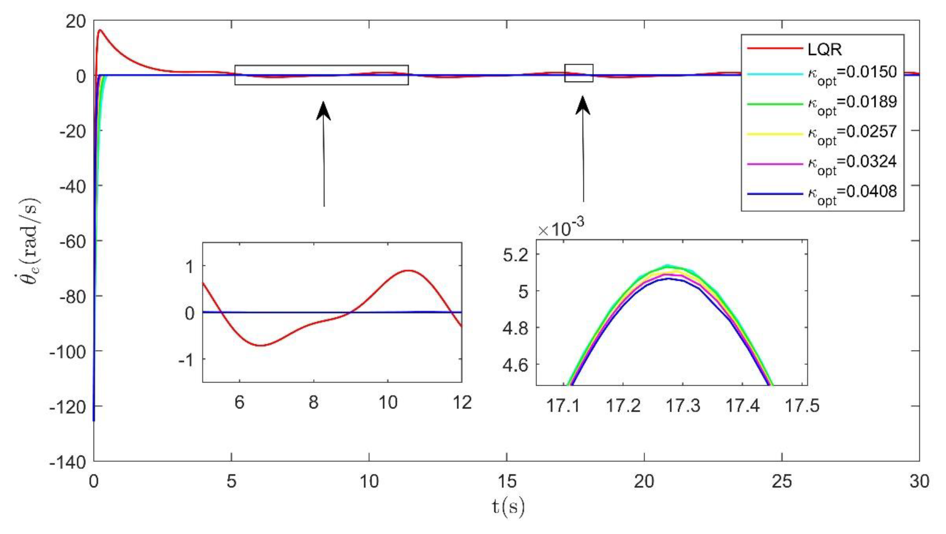
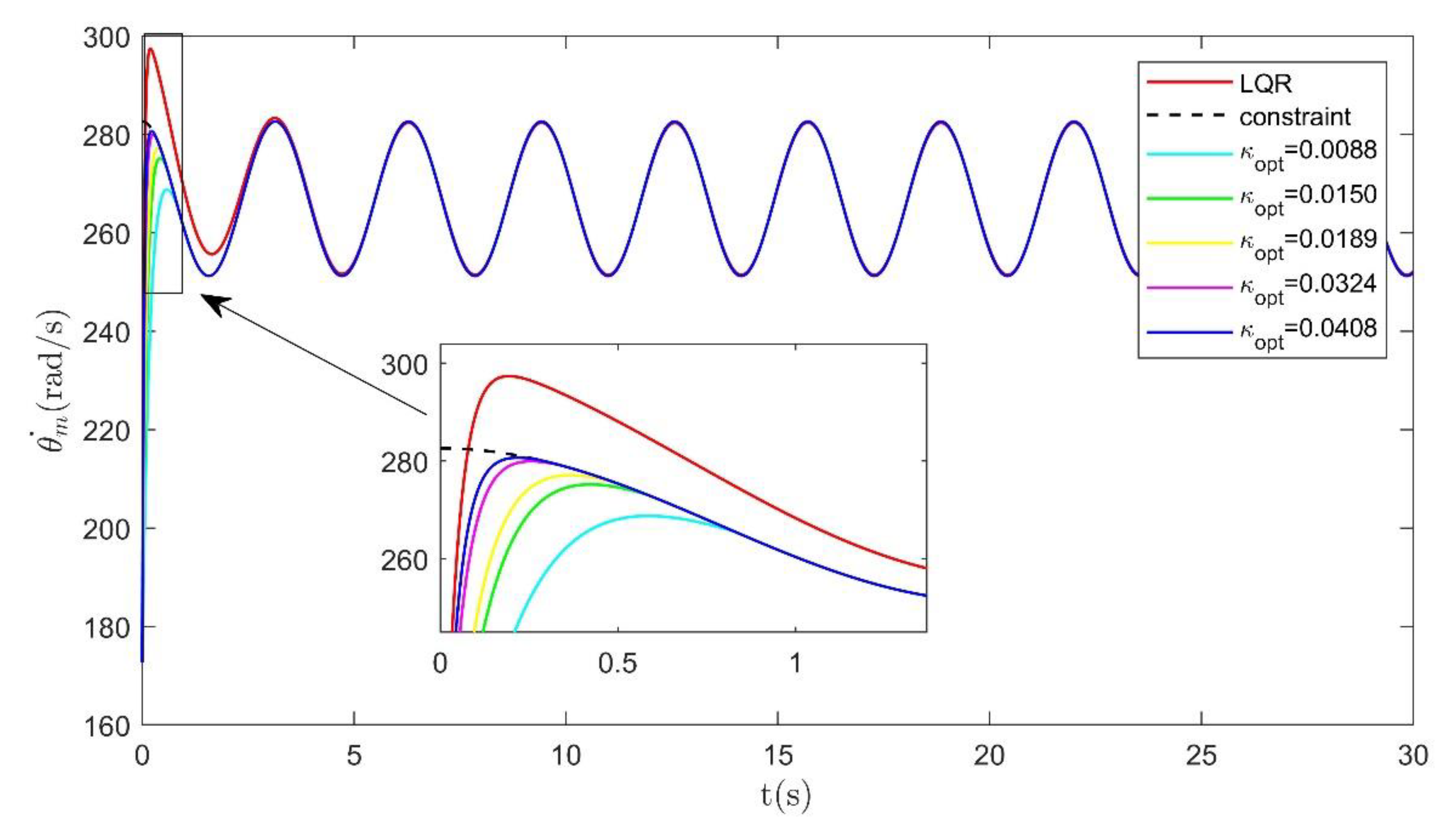
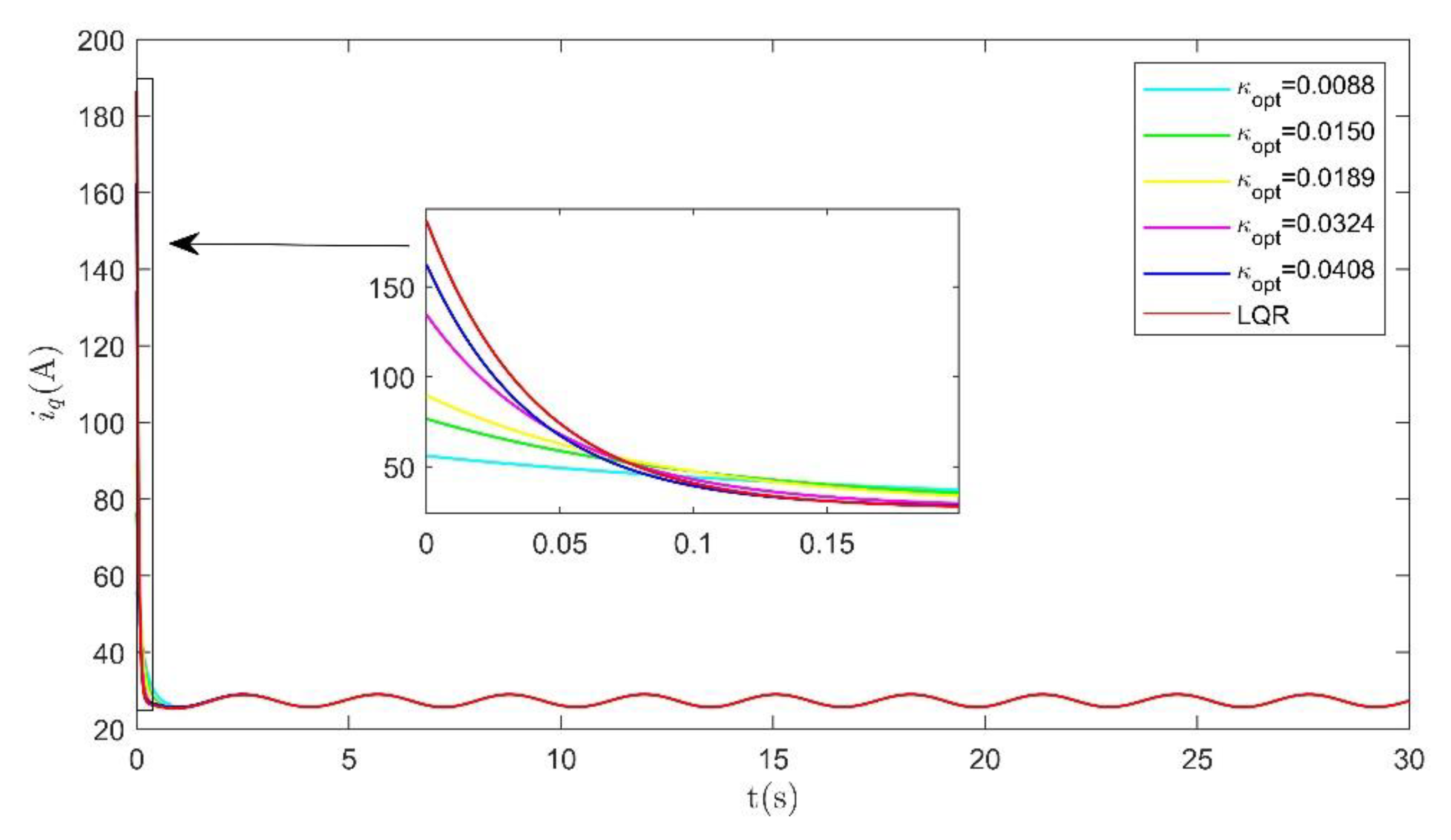
5.1. Step Response under Variable Load Condition

Figure 2 shows the power variation of the main rotor from hovering state to high-speed horizontal forward flight of the helicopter at a height of 100 m. Figure 2 shows that the total power ${{\displaystyle P}}_M$ is ‘saddle shaped’ with the horizontal forward flight speed $V$ (the relation between $V$ and $t$ is $\dot{V}(t)=1$), which basically conforms to the actual working conditions (when the horizontal forward flight speed $V$ is less than the induced speed of helicopter hovering ${{\displaystyle V}}_h$, the helicopter induced speed is considered as induced speed of helicopter hovering).

Figure 3 shows the variation of tail rotor load ${{\displaystyle T}}_t$ and equivalent load ${{\displaystyle T}}_{tr}$ with the horizontal forward flight speed $V$.

We set the tracking speed (system constraint) ${{\displaystyle \dot{\theta }}}_d=90\pi (rad/s)$ and initial speed ${{\displaystyle \dot{\theta }}}_{m0}=50\pi (rad/s)$ of the electric tail reduction system. The tracking speed error in the simulation was defined as ${{\displaystyle \dot{\theta }}}_e={{\displaystyle \dot{\theta }}}_m-{{\displaystyle \dot{\theta }}}_d$. The load of tail rotor followed the actual working conditions in Figure 2 and Figure 3. Here, it was assumed that the helicopter flies forward horizontally without yaw demand (i.e., ${{\displaystyle M}}_f=0$). Based on Assumption 2, we chose $A=1$,$b=0$. In (29), we chose $n=4$, then the robust control gain can be expressed as

$$\gamma (||\mu ||)=\frac{{{\displaystyle (1+{{\displaystyle \widehat{\rho }}}_E)}}^{-1}{{\displaystyle ||\mu ||}}^2}{||\overline{\mu }||({{\displaystyle ||\mu ||}}^3+{{\displaystyle ||\mu ||}}^2\epsilon +||\mu ||{{\displaystyle \epsilon }}^2+{{\displaystyle \epsilon }}^3)}$$

We chose $\epsilon =1$, $P=1$. By choosing five different $\widehat{\alpha }$’s, their values and the corresponding ${{\displaystyle \kappa }}_{opt}$’s and ${{\displaystyle J}}_{\min }$’s are given in

Table 2. Weighting factor/optimal parameter/minimum performance index.

$\widehat{\mathit{\alpha }}$	${{\displaystyle \mathit{\kappa }}}_{\mathbf{opt}}$	${{\displaystyle \mathit{J}}}_{\mathbf{min}}$
100/10	0.0150	0.0068
50/10	0.0189	0.0054
20/10	0.0257	0.0040
10/10	0.0324	0.0031
5/10	0.0408	0.0025

. In (25), $\Delta {{\displaystyle J}}_{tr}=0.02\sin (t)$, $\Delta {{\displaystyle B}}_{tr}=0.001\cos (2t)$ and $\Delta {{\displaystyle T}}_{tr}=\sin (t)$ are used to simulate uncertainty and load disturbance of system. Furthermore, according to (32), we chose the bounding function $\rho =55$.

Figure 4, Figure 5 and Figure 6 show the simulation results under variable tail rotor load including the effects of five different optimized ${{\displaystyle \kappa }}_{opt}$ on system performance. Compared with the LQR control, Figure 4 shows that the robust constraint following control method proposed in this paper has faster response to the system and can approach the constraint in a shorter time. Figure 5 shows that when the control precision was higher, with the increase of design parameter ${{\displaystyle \kappa }}_{opt}$, the tracking error decreased gradually. Figure 6 shows that the method can satisfy the constraints with less maximum control cost under the condition of ensuring the control accuracy of the system. For different optimization parameters ${{\displaystyle \kappa }}_{opt}$, the system response was the fastest and the control precision was the highest when ${{\displaystyle \kappa }}_{opt}=0.0408$, but the control cost was the largest, and then the minimum performance index ${{\displaystyle J}}_{\min }$ was the smallest. Under LQR control, it took several seconds for the tail rotor speed to converge to the expected speed, and the overall error was relatively large.

Figure 2, Figure 3, Figure 4, Figure 5 and Figure 6 show that with the increase in helicopter horizontal forward flight speed, the required control cost of electric tail reduction system first increased slightly (high induced power at low speed), then decreased, and then increased when the tail rotor speed did not change.

5.2. Sinusoidal Response under Constant Load Condition

We set the tracking speed (system constraint) ${{\displaystyle \dot{\theta }}}_d=85\pi +5\pi \cos (2t)(rad/s)$ and initial speed ${{\displaystyle \dot{\theta }}}_{m0}=55\pi (rad/s)$ of the electric tail reduction system. The tracking speed error in the simulation was defined as ${{\displaystyle \dot{\theta }}}_e={{\displaystyle \dot{\theta }}}_m-{{\displaystyle \dot{\theta }}}_d$. In this section, when $V={{\displaystyle V}}_h$, the tail rotor load was ${{\displaystyle T}}_{tr}=19.4692(Nm)$.

Taking the first-order derivative of the above constraint with respect to $t$, in accordance with (23), then $A=1$, $b=-10\pi \sin (2t)$. In (29), we chose $n=4$, then the robust control gain can be expressed as

$$\gamma (||\mu ||)=\frac{{{\displaystyle (1+{{\displaystyle \widehat{\rho }}}_E)}}^{-1}{{\displaystyle ||\mu ||}}^2}{||\overline{\mu }||({{\displaystyle ||\mu ||}}^3+{{\displaystyle ||\mu ||}}^2\epsilon +||\mu ||{{\displaystyle \epsilon }}^2+{{\displaystyle \epsilon }}^3)}$$

We chose $\epsilon =1$, $P=1$. By choosing five different $\widehat{\alpha }$’s, their values and the corresponding ${{\displaystyle \kappa }}_{opt}$’s and ${{\displaystyle J}}_{\min }$’s are given in

Table 3. Weighting factor/optimal parameter/minimum performance index.

$\widehat{\mathit{\alpha }}$	${{\displaystyle \mathit{\kappa }}}_{\mathbf{opt}}$	${{\displaystyle \mathit{J}}}_{\mathbf{min}}$
500/10	0.0088	0.0116
100/10	0.0150	0.0068
50/10	0.0189	0.0054
10/10	0.0324	0.0031
5/10	0.0408	0.0025

. In (25), $\Delta {{\displaystyle J}}_{tr}=0.002\sin (t)$, $\Delta {{\displaystyle B}}_{tr}=0.001\cos (2t)$, and $\Delta {{\displaystyle T}}_{tr}=0.05\cos (t)$ are used to simulate uncertainty and load disturbance of the system. Furthermore, according to (32), we chose the bounding function $\rho =15$.

Figure 7, Figure 8 and Figure 9 show the simulation results under the maximum rotor load at low speed flight conditions including the effects of five different optimization schemes on system performance. Compared with the LQR control, Figure 7 shows that the proposed robust constraint tracking control method had a faster response to the system and could approach the constraint in a shorter time, however, it took about 3 s for LQR control to approach the constraint. Figure 8 shows that the control accuracy of the robust constraint following the control method was relatively higher, and the tracking error was closer to zero. Figure 9 shows that this method can satisfy the constraint conditions with less maximum control cost under the premise of ensuring the control accuracy of the system. For different control parameters ${{\displaystyle \kappa }}_{opt}$, when $\widehat{\alpha }$ was smaller, ${{\displaystyle \kappa }}_{opt}$ was larger, and ${{\displaystyle J}}_{\min }$ was smaller. With the increase in ${{\displaystyle \kappa }}_{opt}$, the response time of the system was shorter, the control accuracy was higher, and the control cost was higher. In the simulation ${{\displaystyle \kappa }}_{opt}=0.0408$, the system response was the fastest, the control precision was the highest, but the control cost was the largest. In contrast, when ${{\displaystyle \kappa }}_{opt}=0.0088$, the system response was the slowest and the maximum control required was minimal.

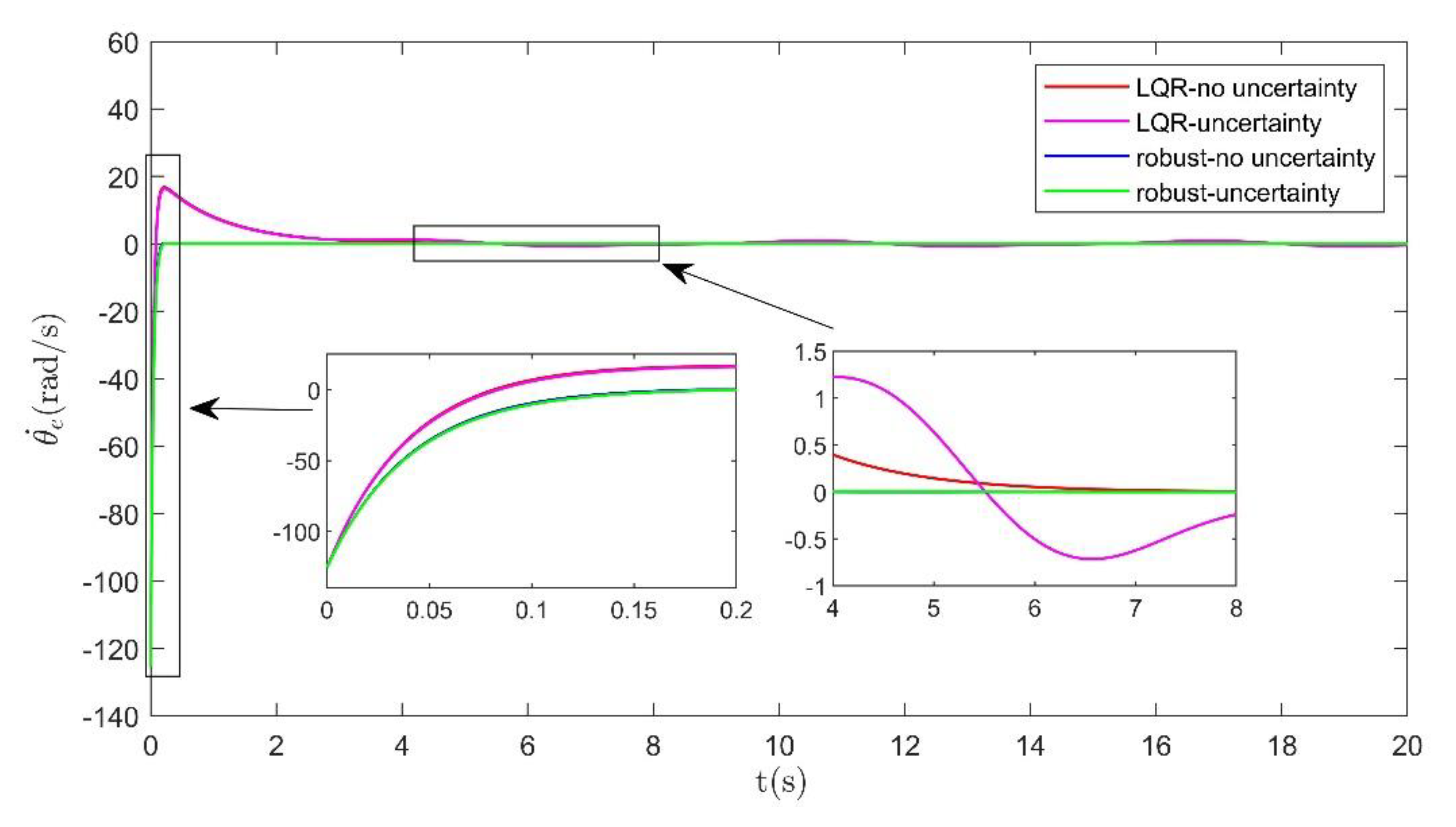
5.3. Tracking Response with Uncertainty or Not

In Section 5.1 and Section 5.2, the different load states, uncertainties, optimization parameters, and the minimum performance indexes are considered. In this part of the simulation, to verify the effect of the proposed control method in dealing with the uncertainty, the tracking response with uncertainty or not is considered. Based on Section 5.1 of the parameter selection and simulation, we chose $\kappa =0.0408$ and initial error ${{\displaystyle \dot{\theta }}}_{e0}=-40\pi (rad/s)$. Figure 10 shows that when there is no uncertainty, the final tracking accuracy of the LQR control and robust constraint following control methods are very high, but the tracking error of LQR control method needs about 5 s to reach zero. When there is uncertainty, the final tracking error of the two methods increased compared with no uncertainty. The tracking error of the LQR control increased greatly (tracking error was about $\pm 0.7$ or so), and the tracking error of robust constraint following control increased little (maximal tracking error was about $6\times {{\displaystyle 10}}^{-3}$ or so). The simulation results showed that the robust constraint following the control method had a strong suppression effect on the uncertainty of the electric tail reduction system. Compared with the traditional LQR control, the proposed method had a faster response and smaller tracking error as well as better transient and steady-state performance.

6. Conclusions

The control of the electric tail reduction system of the unmanned helicopter has certain complexity, mainly due to uncertainty in the system, which is a typical uncertain mechanical system. In this paper, the dynamic model of the electric tail reduction system was established. Considering the flight state and main rotor condition of the helicopter, the tail rotor load of the electric tail reduction system was described from the perspective of flight state. A robust constraint following control method based on the Udwadia–Kalaba theory was proposed to guarantee the deterministic system performance: uniform boundedness and uniform ultimate boundedness. Numerical simulation results showed that the proposed method could deal with the system uncertainty well, and basically met the performance requirements of faster response, smaller error fluctuation, and lower maximum control cost. In addition, a performance index minimization method was proposed to solve the optimization design problem of the control parameter, and the unique solution of the optimal parameter was obtained.

References

1. Alvarenga, J.; Vitzilaios, N.I.; Valavanis, K.P.; Rutherford, M.J. Survey of unmanned helicopter model-based navigation and control techniques. J. Intell. Robot. Syst. 2015, 80, 87–138. [Google Scholar] [CrossRef]
2. Kendoul, F. Survey of advances in guidance, navigation, and control of unmanned rotorcraft systems. J. Field Robot. 2012, 29, 315–378. [Google Scholar] [CrossRef]
3. Zhang, Y.; Jiang, C.; Yunjie, W.A.; Fan, S.U.; Haowen, W.A. Design and application of an electric tail rotor drive control (ETRDC) for helicopters with performance tests. Chin. J. Aeronaut. 2018, 31, 1894–1901. [Google Scholar] [CrossRef]
4. Zhou, J.; Khot, L.R.; Peters, T.; Whiting, M.D.; Zhang, Q.; Granatstein, D. Efficacy of unmanned helicopter in rainwater removal from cherry canopies. Comput. Electron. Agric. 2016, 2016, 161–167. [Google Scholar] [CrossRef] [Green Version]
5. Ma, R.; Ding, L.; Wu, H. Dynamic decoupling control optimization for a small-scale unmanned helicopter. J. Robot. 2018, 2018, 9897684. [Google Scholar] [CrossRef] [Green Version]
6. Sheng, Z.; Li, Y. Hybrid Robust Control Law with Disturbance Observer for High-Frequency Response Electro-Hydraulic Servo Loading System. Appl. Sci. 2016, 6, 98. [Google Scholar] [CrossRef] [Green Version]
7. Li, R.; Chen, M.; Wu, Q. Robust control for an unmanned helicopter with constrained flapping dynamics. Chin. J. Aeronaut. 2018, 31, 2136–2148. [Google Scholar] [CrossRef]
8. Sheng, S.; Sun, C. Design of a Stability Augmentation System for an Unmanned Helicopter Based on Adaptive Control Techniques. Appl. Sci. 2015, 5, 575–586. [Google Scholar] [CrossRef] [Green Version]
9. Yan, K.; Chen, M.; Wu, Q.; Wang, Y. Adaptive flight control for unmanned autonomous helicopter with external disturbance and actuator fault. J. Eng. 2019, 2019, 8359–8364. [Google Scholar] [CrossRef]
10. Yan, K.; Wu, Q.X.; Chen, M. Robust adaptive backstepping control for unmanned autonomous helicopter with flapping dynamics. In Proceedings of the 2017 13th IEEE International Conference on Control & Automation (ICCA), Ohrid, Macedonia, 3–6 July 2017; pp. 1027–1032. [Google Scholar]
11. Chen, N.; Huang, J.; Zhou, Y. Adaptive sliding mode for path following control of the unmanned helicopter based on disturbance compensation techniques. In Proceedings of the 2017 29th Chinese Control and Decision Conference (CCDC), Chongqing, China, 28–30 May 2017; pp. 2670–2677. [Google Scholar]
12. Suzuki, S.; Nakazawa, D.; Nonami, K.; Tawara, M. Attitude control of small electric helicopter by using quaternion feedback. J. Syst. Des. Dyn. 2011, 5, 231–247. [Google Scholar] [CrossRef] [Green Version]
13. Jiang, T.; Lin, D.; Song, T. Finite-time control for small-scale unmanned helicopter with disturbances. Nonlinear Dyn. 2019, 96, 1–17. [Google Scholar] [CrossRef]
14. Mu, D.; Wang, G.; Fan, Y.; Bai, Y.; Zhao, Y. Fuzzy-based optimal adaptive line-of-sight path following for underactuated unmanned surface vehicle with uncertainties and time-varying disturbances. Math. Probl. Eng. 2018, 2018, 7512606. [Google Scholar] [CrossRef] [Green Version]
15. Wang, K.; Rong, H.; Shi, M.; Meng, Z.; Zhou, Y. Reactive obstacle avoidance for unmanned helicopter using fuzzy control. In Proceedings of the 37th Chinese Control Conference, Wuhan, China, 25 July 2018; pp. 10026–10031. [Google Scholar]
16. Yuan, Y.; Thomson, D.; Chen, R.L.; Dunlop, R. Heading control strategy assessment for coaxial compound helicopters. Chin. J. Aeronaut. 2019, 32, 2037–2046. [Google Scholar] [CrossRef]
17. Han, D.; Barakos, G.N. Variable-speed tail rotors for helicopters with variable-speed main rotors. Aeronaut. J. 2017, 121, 433–448. [Google Scholar] [CrossRef] [Green Version]
18. Rajendran, S.; Gu, D.W. Fault tolerant control of a small helicopter with tail rotor failures in forward flight. IFAC Proc. Vol. 2014, 47, 8843–8848. [Google Scholar] [CrossRef]
19. Fletcher, T.M.; Brown, R.E. Main rotor-tail rotor interaction and its implications for helicopter directional control. J. Am. Helicopter Soc. 2008, 53, 125–138. [Google Scholar] [CrossRef] [Green Version]
20. Truong, H.V.A.; Tran, D.T.; To, X.D.; Ahn, K.K.; Jin, M. Adaptive Fuzzy Backstepping Sliding Mode Control for a 3-DOF Hydraulic Manipulator with Nonlinear Disturbance Observer for Large Payload Variation. Appl. Sci. 2019, 9, 3290. [Google Scholar] [CrossRef] [Green Version]
21. Iqbal, J.; Zuhaib, K.M.; Han, C.; Khan, A.M.; Ali, M.A. Adaptive Global Fast Sliding Mode Control for Steer-by-Wire System Road Vehicles. Appl. Sci. 2017, 7, 738. [Google Scholar] [CrossRef]
22. Udwadia, F.E.; Kalaba, R.E. A new perspective on constrained motion. Proceedings of the Royal Society. Math. Phys. Sci. 1992, 439, 407–410. [Google Scholar]
23. Kalaba, R.E.; Udwadia, F.E. Lagrangian mechanics, Gauss’s principle, quadratic programming, and generalized inverses: New equations for nonholonomically constrained discrete mechanical systems. Q. Appl. Math. 1994, 52, 229–241. [Google Scholar] [CrossRef] [Green Version]
24. Udwadia, F.E.; Kalaba, R.E. Analytical Dynamics: A New Approach; Cambridge University Press: Cambridge, UK, 1996. [Google Scholar]
25. Udwadia, F.E.; Kalaba, R.E. Explicit equations of motion for mechanical systems with nonideal constraints. J. Appl. Mech. 2001, 68, 462–467. [Google Scholar] [CrossRef] [Green Version]
26. Udwadia, F.E. A new perspective on the tracking control of nonlinear structural and mechanical systems. Math. Phys. Eng. Sci. 2003, 459, 1783–1800. [Google Scholar] [CrossRef] [Green Version]
27. Chen, Y. Equations of motion of mechanical systems under servo constraints: The Maggi approach. Mechatronics 2008, 18, 208–217. [Google Scholar] [CrossRef]
28. Zhao, H.; Zhen, S.; Chen, Y. Dynamic modeling and simulation of multi-body systems using the Udwadia-Kalaba theory. Chin. J. Mech. Eng. 2013, 26, 839–850. [Google Scholar] [CrossRef]
29. Sun, H.; Zhao, H.; Zhen, S.; Huang, K.; Zhao, F.; Chen, X.; Chen, Y.H. Application of the Udwadia-Kalaba approach to tracking control of mobile robots. Nonlinear Dyn. 2016, 2016, 389–400. [Google Scholar] [CrossRef]
30. Sun, H.; Zhao, H.; Huang, K.; Qiu, M.; Zhen, S.; Chen, Y.H. A fuzzy approach for optimal robust control design of automotive electronic throttle system. IEEE. Trans. Fuzzy Syst. 2018, 26, 694–704. [Google Scholar] [CrossRef]
31. Li, C.; Chen, Y.H.; Sun, H.; Zhao, H. Optimal design of high-order control for fuzzy dynamical systems based on the cooperative game theory. IEEE. Trans. Cybern. 2020, 2020, 1–10. [Google Scholar] [CrossRef]
32. Li, C.; Zhao, H.; Sun, H.; Chen, Y. Robust bounded control for nonlinear uncertain systems with inequality constraints. Mech. Syst. Signal Process. 2020, 140, 106665. [Google Scholar] [CrossRef]
33. Dong, F.; Chen, Y.; Zhao, X. Optimal design of adaptive robust control for fuzzy swarm robot systems. Int. J. Fuzzy Syst. 2019, 21, 1059–1072. [Google Scholar] [CrossRef]
34. Sun, H.; Yu, R.; Chen, Y.; Zhao, H. Optimal design of robust control for fuzzy mechanical systems: Performance-based leakage and confidence-index measure. IEEE. Trans. Fuzzy Syst. 2019, 27, 1441–1455. [Google Scholar] [CrossRef]
35. Chen, Y. Second-order constraints for equations of motion of constrained systems. IEEE/ASME Trans. Mechatron. 1998, 3, 240–248. [Google Scholar] [CrossRef]
36. Maxwell, J.C. A treatise on electricity and magnetism 2. Nature 2010, 7, 478–480. [Google Scholar]
37. Newman, S.J. Methods of Calculating Helicopter Power, Fuel Consumption and Mission Performance; Technical Report; University of Southampton: Southampton, UK, 2011. [Google Scholar]
38. Chen, Y.; Zhang, X. Adaptive robust approximate constraint-following control for mechanical systems. J. Frankl. Inst. 2010, 347, 69–86. [Google Scholar] [CrossRef]
39. Zhao, X.; Chen, Y.; Zhao, H.; Dong, F. Udwadia-Kalaba Equation for Constrained Mechanical Systems: Formulation and Applications. Chin. J. Mech. Eng. 2018, 31, 106. [Google Scholar] [CrossRef] [Green Version]
40. Zhen, S.; Huang, K.; Sun, H.; Zhao, H.; Chen, Y. Dynamic modeling and optimal robust approximate constraint following control of constrained mechanical systems under uncertainty: A fuzzy approach. J. Intell. Fuzzy Syst 2015, 2015, 777–789. [Google Scholar] [CrossRef]
41. Chen, Y. On the deterministic performance of uncertain dynamical systems. Int. J. Control 1986, 43, 1557–1579. [Google Scholar] [CrossRef]
Figure 1. Electric tail reduction system.
Applsci 11 00260 g001
Figure 2. The main rotor power varying with the helicopter horizontal forward speed.
Applsci 11 00260 g002
Figure 3. The tail rotor load varying with the helicopter horizontal forward speed.
Applsci 11 00260 g003
Figure 4. The step tracking speed curve of the electric tail reduction system.
Applsci 11 00260 g004
Figure 5. The step tracking speed error curve of the electric tail reduction system.
Applsci 11 00260 g005
Figure 6. The step tracking control cost curve of the electric tail reduction system.
Applsci 11 00260 g006
Figure 7. The sinusoidal tracking speed curve of the electric tail reduction system.
Applsci 11 00260 g007
Figure 8. The sinusoidal tracking speed error curve of the electric tail reduction system.
Applsci 11 00260 g008
Figure 9. The sinusoidal tracking control cost curve of the electric tail reduction system.
Applsci 11 00260 g009
Figure 10. The step tracking speed error curve with uncertainty or not.
Applsci 11 00260 g010