Abstract
Featured Application
Remote handling of ITER’s divertor cassette locking system.
Abstract
Visual technologies have an indispensable role in safety-critical applications, where tasks must often be performed through teleoperation. Due to the lack of stereoscopic and motion parallax depth cues in conventional images, alignment tasks pose a significant challenge to remote operation. In this context, machine vision can provide mission-critical information to augment the operator’s perception. In this paper, we propose a retro-reflector marker-based teleoperation aid to be used in hostile remote handling environments. The system computes the remote manipulator’s position with respect to the target using a set of one or two low-resolution cameras attached to its wrist. We develop an end-to-end pipeline of calibration, marker detection, and pose estimation, and extensively study the performance of the overall system. The results demonstrate that we have successfully engineered a retro-reflective marker from materials that can withstand the extreme temperature and radiation levels of the environment. Furthermore, we demonstrate that the proposed maker-based approach provides robust and reliable estimates and significantly outperforms a previous stereo-matching-based approach, even with a single camera.
1. Introduction
Visual technologies have been increasingly integrated into industrial contexts with the intent of increasing work turnover, repeatability, or operator safety [,]. In safety-critical contexts, where operator access is restricted and tasks need to be performed through teleoperation, such as space, underwater exploration, mining, and nuclear reactors [], these technologies have a particularly indispensable role. This is true especially in large-scale applications with many dynamic elements, where the current status of the system cannot be modeled accurately.
For safe and effective task performance, operators should have full situational awareness of the current status of the remote environment, especially during fine alignment tasks, where the operator has to position the manipulator in a certain position and orientation in relation to a target object with a high degree of accuracy. These tasks can represent a particular challenge for teleoperation due to the lack of some of the natural depth cues in standard image or video feedback [,].
In this context, machine vision approaches can be used to extract and refine mission-critical information from the images, such as the relative position between the tool and the target, which can be used as a teleoperation aid. This type of teleoperation aid has been successfully used for maintenance and assembly tasks in extra-vehicular space applications []. In the aforementioned work, the computed six degrees of freedom (DOF) transformation between the current and desired end-effector positions is overlaid on the camera feed showed to the operator as either graphics or text.
The application that motivated our work is remote handling of ITER’s (https://www.iter.org/) divertor cassette locking system. ITER constitutes one of the world’s most hostile remote handling environments and is characterized by the unpredictable nature of its maintenance situations and tasks []. In ITER, all tasks are to be performed using a human-in-the-loop telemanipulation approach where the operator is always in control, although remotely located to minimize the risk of ionizing radiation exposure []. Operation in this environment differs from a common industrial environment, since high radiation levels and temperatures and strong magnetic fields strictly limit the materials that can be used in the activated areas, including the hardware that can be used for sensing the environment. This deems necessary the use of radiation-tolerant cameras, which are often characterized by a low resolution, gray-scale output, and high level of noise, which degrades with exposure to radiation over the lifetime of the camera. The operation of the divertor cassette locking system requires the alignment of several tools to their respective slots. Both the tools and the manipulator are carried in by a transporter that moves on rails throughout the facility. The tolerances for error in tool-slot alignment are small, with ±3 mm of maximum allowed error in translation. Taking into account the difficulty in making a visual alignment in this range, there is a need to develop an accurate machine-vision-based aid that can comply with the strict requirements of the application.
Our aim here is to develop a system that calculates, using a set of one or two cameras attached to the wrist of the robotic manipulator, the transformation between the robot end-effector and the target (cassette). This information is intended to be used to update the models behind the virtual-reality-based remote handling platform [,].
Most man-made structures in the ITER environment, like the divertor cassettes, have large, flat, textureless surfaces, which are often specularly reflective and look different from different perspectives. Such surfaces pose a challenge to conventional 3D reconstruction algorithms that require the establishment of robust feature correspondences across multiple images. In a previous work [,], some of these challenges have been circumvented by extracting edge information from images provided by an array of two cameras as a prior step to stereo matching. The system obtains a relatively sparse 3D representation of the scene that is, at a later stage, matched with the known 3D model of the cassette to calculate the six-DOF transformation between the camera and the target. We consider the aforementioned approach to be sub-optimal for the application, since it does not explicitly exploit the prior knowledge of the structure of the environment at the feature detection and geometry reconstruction stages. As a result, this earlier solution is not as robust or accurate as required for the application at hand. We hypothesize that more reliable results can be achieved by detecting the known features of the cassette, or, even better, through the introduction of marker objects in the cassette surface that can be tracked by cameras unambiguously and accurately. Furthermore, there is a need, due to space constraints, to reduce the number of cameras to just one while still maintaining the targeted high-accuracy target pose estimation.
Marker-based tracking has been used in human motion analysis [], medicine [], and augmented reality [,,] applications, localization of wearables [], and in unmanned aerial vehicle and robot navigation systems [,,,]. It has also been used in industrial contexts [], such as component inspection and validation [,]. It can obtain significantly superior results compared to tracking natural features, particularly when objects in the scene have limited contrast features, have few identifiable features, or change appearance with viewpoint [,]. Marker objects used for tracking can be LEDs, white diffuse markers, light projected targets, or retro-reflective markers [].
A retro-reflector is an optical element that returns light to its source for a wide range of incident directions. They are best known for their use in traffic safety, where they improve visibility under poor light conditions by returning incoming headlamp light in a small cone that covers the viewpoint of the driver. The intensity of retro-reflected light in the direction of the source can be up to hundreds to even thousands of times higher than that of a diffuse target []. They have also been used together with a laser for making distance measurements in space [], industrial [], and robotics applications [].
In photogrammetry, retro-reflective markers allow the production of an almost binary image by controlling image exposure in such a way that the background is under-exposed and largely eliminated []. This process has advantages in target recognition and extraction, high-precision locating, and noise suppression [].
As the above-mentioned characteristics deem retro-reflective markers optimal for the ITER application, in this paper, we aim to design a retro-reflective marker setting that complies with the strict requirements of such environment and can be attached to the surface of the cassettes for their effective tracking. We develop and test a system that uses said markers to reliably estimate the alignment between a pin-tool and the respective slots in the cassette surface.
The concept has previously been presented on a system level to the fusion engineering community []. Here, we detail it from a machine vision perspective with the following contributions:
- A marker design that complies with the extremely strict requirements set by the operating environment.
- A methodology for marker detection and correspondence and optimization of the estimated pose.
- An approach for remote calibration of radiation-activated cameras.
- A study of the performance of monocular versus stereoscopic pose estimation on synthetically generated data with varying baselines.
- A comprehensive prototype implementation of the system and thorough evaluation of its overall performance.
The paper is organized as follows: In Section 2, we detail our proposed methods. In Section 3, we present the results of an extensive study of the performance of the system and a comparison to the earlier solution. In Section 4, we present our concluding remarks and outline future development prospects.
2. Methods
In the terminology of this paper, T represents a homogeneous rigid body transformation between two coordinate frames, which can be written as follows: , where R represents the 3 × 3 rotation matrix and t represents the 3 × 1 translation vector. The main coordinate frames and transformations that will be referenced throughout the work are represented in Figure 1.
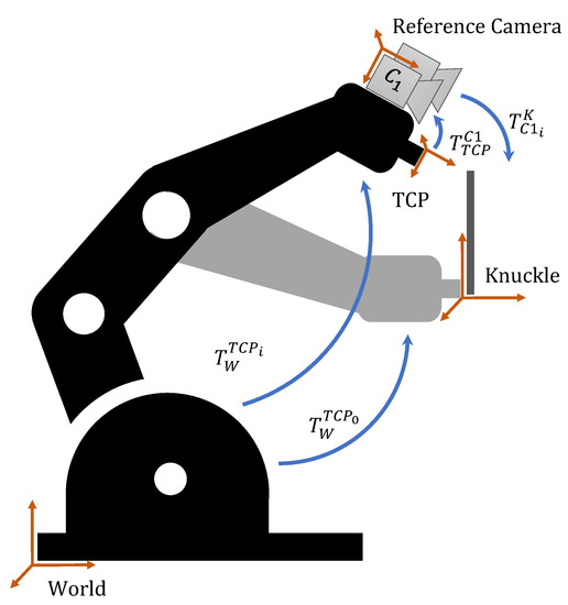
Figure 1.
Relevant coordinate frames and rigid body transformations.
Here, represents the transformation from the robot-base coordinate frame to the robot’s tool center point (TCP) that is given at each position i by the robot’s control system (CS). represents the transformation between the robot’s TCP and the attached reference camera that is independent of the position of the manipulator and is obtained through a hand–eye calibration procedure. represents the transformation between the reference camera and a reference point in the world (e.g., origin of a target) at each position i. represents the transformation between the robot base and the TCP when the TCP and target coordinate systems coincide, i.e., the aligned position.
2.1. Retro-Reflective Marker Design
Retro-reflectors can be characterized by four main properties: retro-reflectance (ratio of retro-reflected to incident light), brilliancy (reflectance for a specific observation angle), divergence (maximum angular distribution of retro-reflected light), and angularity (brilliancy as a function of the incident angle) []. In many applications, the desired marker behavior resembles the ideal retro-reflector, which allows large entrance angles (high angularity) and returns as much light as possible in as small a cone of light as possible (high reflectance, high brilliancy, and low divergence). However, in applications where there is a displacement between the light source and the detector, higher divergence might be acceptable or even required. As an example, in traffic applications, where there is a displacement between the car’s headlamps and the driver’s eyes of about 60 cm, the useful retro-reflecting angle has been quantified to be from nearly 0 to approximately 3 degrees for distances of 12 to 122 m []. In this case, the aim is to optimize brilliancy at the observation angle rather than at the incident angle. This is often achieved by using a retro-reflector with higher divergence, though at the cost of some intensity loss.
The same principle applies to photogrammetry and dictates the first functional requirement of an effective retro-reflector for our application. The useful retro-reflecting angle can be easily quantified for a specific setup as a function of the imaging distance (H) and the displacement between the camera and the light source (D) as follows:
For the setup used in this work, we calculate a maximum useful retro-reflecting angle of ±18 for the shortest working distance and the maximum possible displacement between the camera and the source.
The second functional requirement of a successful retro-reflector is the acceptance angle. We consider that an acceptance angle of ±10 is sufficient for our application, since an operator can, with very little effort, make a preliminary target alignment within this range. Furthermore, there is no minimum specification for the retro-reflectance, but the aim is to maximize its value.
There is a relatively long list of environment requirements dictated by the ITER application when it comes to materials that stay in the divertor for a considerable amount of time. These include an operating temperature of up to 200 C and adequate radiation tolerance. In practice, these restrictions deem unfeasible the use of most common materials, except for stainless steel (which makes up most of the other structures in the divertor) and fused silica glass (which is planned to be used in diagnostic windows and fiber optics). To the best of our knowledge, there is no adhesive material that can be used in this environment. Furthermore, the size of the developed marker should be rather small, such that the mounting of several specimens in a 200 × 200 mm area is feasible and the embedment depth should be rather small so as not to compromise the structural integrity of the cassette.
Retro-reflection is often achieved using one of two designs: a corner cube or a lens and a mirror. Corner-cube retro-reflectors (CCR) rely on the reflection of light on three mutually orthogonal surfaces. Generally, CCRs are manufactured either as a truncated cube corner of a transparent material (i.e., prism) or as flat reflective surfaces surrounding empty space. Cat’s eye retro-reflectors consist of a primary lens with a secondary mirror located at its focus []. These can be easily implemented using a sphere of a transparent material. Spherical retro-reflectors generally have higher divergence due to spherical aberration and lower retro-reflectivity. On the other hand, corner-cube retro-reflectors usually have higher retro-reflectivity, while their fabrication is more difficult [,].
A retro-reflective marker can consist of a single shape or an array of retro-reflective shapes of smaller dimensions. The advantage of an array-based pattern is that the depth of the marker can be smaller and the shape of the overall retro-reflective region can be tailored. Furthermore, whilst the shape of the retro-reflective area changes with viewing angle for single-shape retro-reflectors, for those composed of arrays of small elements, the shape is independent of the orientation of the marker. On the other hand, such a construction might be more difficult to implement, as it requires a more precise manufacturing process with tighter tolerances.
In a preliminary study conducted to determine the viability of off-the-shelf retro-reflectors for use in ITER, we found that the only viable solution belonged to the single-element prism category (Edmund Optics BK-7 glass prism). No ready-made markers were found in the corner-cube array or bead array categories that could be used in our application.
Therefore, we propose a custom-made solution consisting of an array of glass beads. Such beads are often used within paint or attached via adhesive to other materials (e.g., paper or plastic). Due to the restriction of using adhesives and paints in ITER environment, the main challenge of using a bead array in our application is their attachment to the surface of the cassette. For this purpose, we propose a custom sieve-like metal holding structure that can hold the beads in place and can be easily mounted into the cassette surface, as illustrated in Figure 2.
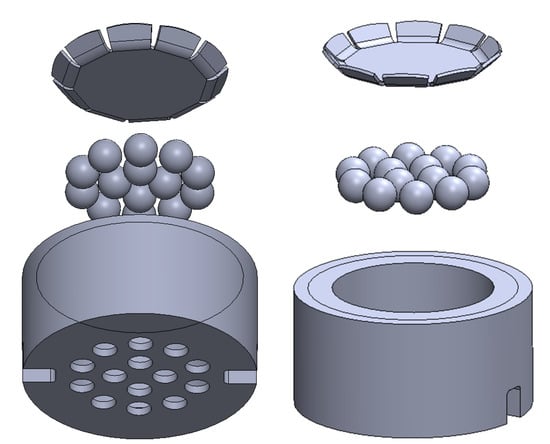
Figure 2.
Retro-reflective bead array marker housing.
Another potential challenge to this approach is that the retro-reflectance of glass beads is quite sensitive to their refractive index (n) [], and the refractive index of fused silica () is relatively low when compared to other glass compositions (). In fact, if we consider the simplest case of a single specular internal reflection from the back of the silica sphere, we can calculate a divergence value of ±25 degrees as follows []:
where h represents the incident height, as shown in the left side of Figure 3, and r represents the radius of the glass bead. In the right side of Figure 3, we show the calculated divergence as a function of the h value.
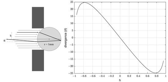
Figure 3.
Incident height (h) and divergence () of light in a retro-reflective bead.
This divergence is higher than required, leading to some loss of intensity. Therefore, this design serves the purposes of the application, even if it does not fully optimize brilliancy at the observation angle. In Figure 4, we illustrate our proposed bead array marker design side by side with the out-of-the-box glass prism, a white diffuse element, and the commonly used bead-based retro-reflective tape that cannot be used for the application, but serves as a reference for a behavior that would be desirable.
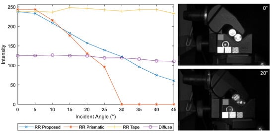
Figure 4.
Illustration of our proposed marker, the off-the-shelf glass prism, retro-reflective tape, and a white diffuse element. Data on the left side of the figure are obtained by averaging the pixel values within the marker area in images taken at several incident angles.
The alternative of manufacturing a stainless steel hollow corner-cube array could technically be implemented and would have the advantage of being made from a single piece and a potentially larger reflective area.
However, while many methods are described in the literature for manufacturing corner-cube arrays [] on both the micro and macro scale, the commercial availability of such methods is still limited and a suitable manufacturer could not be found. Some customized manufacturing methods were considered, mainly consisting of producing a strong enough inverse tool that could emboss the desired pattern onto a stainless steel piece using a hydraulic press. The advantage of this approach would be the flexibility of producing multiple marker specimens at a fixed cost and the fact that the markers could be a single piece made from a single material. However, a suitable method for manufacturing the pressing tool proved hard to find. We considered manufacturing by electrical discharge machining (EDM). However, the surface finish of the tool was quite rough, and the manufacturing tolerances reduced the sharpness of the corners to a curvature with a diameter of approximately 2.0 mm. Furthermore, when pressing the tool onto the metal to create the retro-reflective pattern, the excess material tends to accumulate between the borders of the corner-cube indentation, leading to relatively large non-retro-reflective flat regions. An alternative option would be to create a single-shape corner-cube inverse tool, which would have to be stamped into the piece multiple times to create an array-like structure. Such a tool can be manufactured with a different technique that allows sharper corners. However, this brings additional practical issues related to the alignment of the tool that diminish the usability of this approach.
We concluded that the most viable and cost-effective solution for the application is the use of the bead-array retro-reflective marker array. The experiments presented further on in this paper were conducted using this design. We create a marker constellation design for the cassette piece, where we aim to maximize the number of markers while keeping the drilling into the piece at an acceptable level. We partially utilize holes that were already in the design of the cassette surface for other purposes. There is no possibility to mount markers at different depths, so all markers are at the same depth plane. Furthermore, we opt not to use coded markers in order to optimize the available bright marker area and due to the fact that the low resolution makes it hard to detect features of smaller dimensions.
2.2. Automatic Offline Calibration Routine
During operation inside the reactor, it is expected that cameras’ calibration parameters will be affected by shocks, vibration, temperature changes, or other unforeseeable environment factors. Even though there are not yet experimental data on how volatile these parameters will be (since the reactor is under construction), there is a definite need to develop reliable methods for calibration of activated cameras (cameras that have been exposed to radiation and, therefore, cannot be in the same environment as the operators at the same time). The developed calibration procedure should happen offline in the hot-cell facility (dedicated area outside of the operating environment to process activated components) and without manual intervention. The method of choice for camera calibration throughout our work is Matlab’s implementation [] of Zhang’s widely known algorithm for photogrammetric camera calibration [] using the distortion model of []. This method relies on a manual calibration image capture step, which means that the operator would have to move the manipulator and the attached cameras in the vicinity of a calibration pattern and capture a minimum of three calibration images at different camera orientations. This is an undesirable, time-consuming, and repetitive procedure with a low level of repeatability, since different manipulator positions provide slightly different calibration results. Some methods have been proposed in the literature for automatizing the image capturing step through the display of virtual targets on a screen []. These methods are, however, not applicable to our application due to the difficulty of introducing additional electronics in the hot-cell facility. Therefore, we developed a calibration routine to be performed autonomously by the robotic arm that produces fairly repeatable results. As a target, we used a checkerboard pattern that was placed in the hot-cell facility prior to the start of the calibration routine. Even though the same procedure could be used to re-calibrate the cameras in the reactor, based on the known relative position of the retro-reflective markers, we did not explore this option, mostly due to the tight space constraints in the environment.
As a preliminary step, we summarize what is established as a good set of calibration images: Even though it is possible to obtain a calibration estimate from a smaller number of images [], it is often recommended to acquire at least 10 images of the calibration pattern at different orientations relative to the camera. The images should be captured at a distance that corresponds roughly to the operating distance so that the pattern is in focus. The positions of the pattern shall be such that:
(1) The checkerboard is at an angle lower than 45 degrees relative to the camera plane. According to the original work [], when tested on synthetic data, the calibration method obtains most accurate estimates when the angle between the calibration target and image plane is higher. However, in real imaging conditions, where blur and distortion must be taken into account, angles close to 45 degrees might compromise the accuracy of corner detection, depending on the size of the checkerboard and the depth of field of the camera-lens system.
(2) Feature points should be detectable on as much of the image frame as possible for adequate estimation of the lens distortion parameters.
In our scenario, additional practical considerations need to be taken into account, such as the work-space limitations of the robotic arm and singularity regions of its joints.
To fulfill the above-mentioned requirements, the developed automatic capture routine moves the camera in discrete positions within a spherical surface centered in the calibration pattern center, as shown in Figure 5. The radius of the spherical surface corresponds, approximately, to the average operating distance.
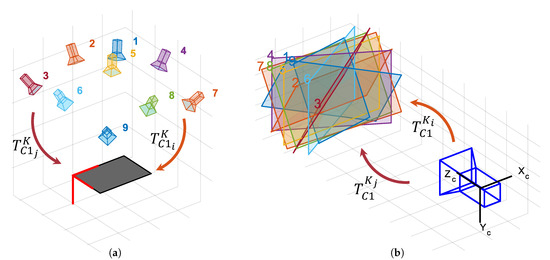
Figure 5.
Camera movement in a dome around the centre of the checkerboard pattern seen from a pattern-centric perspective (a) and from a camera centric perspective (b).
The camera rotations are such that the center of the pattern is kept in the center of the image plane. The described movement is equivalent to the rotation of the calibration pattern around its center in each of the three rotation dimensions (yaw, pitch, and roll) in a camera-centric interpretation of the problem. For the sake of simplicity, we calculate the desired camera-to-target transformations () using the camera-centric interpretation:
The base-to-end-effector transformations that bring the camera to the desired calibration positions are calculated in the following manner:
where represents a rough estimate of the hand–eye calibration. represents the initial position reported by the robot’s CS and represents the initial transforming between the camera and the target and is estimated from a single image based on nominal values of the camera calibration parameters. The calibration procedure runs automatically. All the operator needs to do is to move the manipulator so that the checkerboard is within the field of view of the camera for the initial pose. At the end of the procedure, the operator will receive a visual representation of the re-projection error indicating whether the procedure was successful. The procedure can be used to capture any desired number of images, and the steps within the range of movement are adapted accordingly.
The captured images are used to calibrate the intrinsic parameters of the cameras and the extrinsic parameters in the case where a stereo pair is used and serve as data for a hand–eye calibration routine. A hand–eye calibration is required for this application in order to align the coordinate systems of the robotic manipulator and the vision system. The details of such a calibration are outside the scope of this paper, and are presented in detail in []. The calibration procedure shall be repeated as needed based on the volatility of the estimated parameters in the real operating conditions.
2.3. Marker Detection and Identification
The preliminary step to position estimation is the determination of correspondences between 2D image features and known 3D world points. The developed marker detection and identification approach is shown in Figure 6.
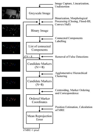
Figure 6.
Workflow of image processing operations leading to marker detection and identification.
It relies on the prior knowledge of the characteristics of the markers and their layout with respect to each other. We perform marker detection and identification independently for each camera image to keep the approach flexible and suitable for the monocular case.
The workflow of marker detection starts with image capture, linearization, and undistortion. Images are segmented into foreground (markers) and background through adaptive thresholding as follows:
Here, represents the value of the resulting binary image at pixel coordinates (x,y), while represents the value of the original gray-scale image at the corresponding coordinate points. represents the median of the w × h surrounding pixels at coordinate (x,y). Adaptive thresholding preserves hard contrast lines while ignoring soft gradient changes. Our approach resembles the methods of []. However, it compares each image pixel to the median of the surrounding pixels, instead of their average, since this approach effectively removes outliers and better preserves details and edges. The value s is a scale factor that contributes to the classification of more or fewer pixels as foreground. We have modified the original method by adding a constant value, T, to the threshold matrix, with the intent of exploiting the fact that the intensity difference between the markers and the background is more significant than in the diffuse marker case. Even though the retro-reflective markers are considerably brighter than their surroundings, the large specular reflections of the cassette surface and some degree of inhomogeneity of the lighting conditions deem advantageous the use of a local thresholding method. However, this has a tendency to increase the number of false blobs detected in the background, which will be handled by morphological filtering. In the following processing steps, several techniques are utilized to determine the suitability of marker candidates. If these point to an incorrect segmentation, the software returns to the thresholding step and the operator is asked to intervene by modifying the threshold parameters in small incremental steps. Decreasing s and/or T will lead to a higher number of pixels being classified as foreground. While manually refining the parameters, the operator is presented with the thresholded image and the result of the overall marker detection pipeline.
After segmentation, each marker is represented by an array of blobs that are merged into a single elliptical shape by applying morphological closing and flood-fill operations [], consecutively followed by determination of the binary convex hull image. The blobs in the resulting image are identified by connected component labeling [] and non-markers are excluded through the comparison of several properties of the connected compound elements to appropriate thresholds. We consider that markers often differ from the remaining blobs with respect to their size (area) and/or and shape (circularity and eccentricity). Circularity is defined by the following ratio:
and has a minimum value of 1 for a circular disk, and is greater than 1 for all other geometric features. For an ellipse, it increases with the imaging angle monotonously and has a value of 1.5 at 60 degree angle []. Eccentricity describes the ratio of the distance between the foci and major axis length of the ellipse that has the same second-moments as the region. It is closer to 0 for a circle-like object, and closer to 1 for a line-like object.
If after the elimination step, the number of identified markers is less than expected, the procedure returns to the segmentation step and prompts the operator to adjust the segmentation parameters.
If after the elimination step, the number of candidate markers is higher than expected, markers are grouped into clusters according to their features, creating an agglomerative hierarchical cluster tree. Selected features are: area, perimeter, circularity, solidity, convex area, equivalent diameter, extent, minimum Feret diameter and maximum, and minimum intensity of the grayscale blob. Solidity describes the extent to which a shape is convex or concave. It corresponds to the ratio between the area and the convex area (area enclosed by a convex hull). The equivalent diameter corresponds to the diameter of a circle with the same area as the region. Extent refers to the ratio of pixels in the region to pixels in the total bounding box. The minimum Feret diameter expresses the minimum distance between any two boundary points on the antipodal vertices of the convex hull that encloses the object. Data values are normalized before computing similarity and the Euclidean distance is used as a distance metric. The hierarchical tree is pruned at the lowest branch, where a class of eight elements can be found. A single feature point is found within each marker by calculating the centroid coordinates ():
where represent the size of the window in which the centroid is being computed and represents the value of the binary image at coordinate . By making the approximation that the centroid of the detected markers corresponds to the center of the original circles, we disregard the perspective bias [] introduced by perspective projection. We assume that the camera and target have been roughly aligned and, consequently, that the value of the perspective bias is rather small.
In order to establish a one-to-one correspondence between the known relative marker positions in the world coordinate frame and the detected image coordinates, the detected markers must be correctly ordered. The proposed marker ordering approach is shown in Figure 7 and finds the line passing through four of the proposed markers. This is achieved by computing all possible combinations of the markers in groups of two (28 groups), fitting a line to each marker pair and finding the six groups of parameters corresponding to the same line using agglomerative hierarchical clustering. The hierarchical cluster tree is pruned at the lowest point, where there is a class composed of five elements. After the line has been determined, the remaining four points can be projected onto the line, and markers can be discriminated from their distance along the line to the origin marker.
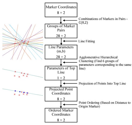
Figure 7.
Workflow of marker ordering.
Pose Estimation
Pose estimation refers to the calculation of the rigid body transformation between the camera and the target () based on a set of detected 2D image points and 3D known world point correspondences.
Pose estimation has been extensively studied in the literature, and many iterative and non-iterative methods have been proposed to solve the problem under different conditions, depending on the number of available point correspondences, presence of outliers, how noisy their coordinates are, whether the problem has to be solved online or offline, and if the camera parameters are known or estimated simultaneously [,,].
In our application, control points are known to be co-planar and are detected with a relatively high degree of accuracy. We use the pose estimate provided by the direct linear transform (DLT) homography estimation method [,] as an initial estimate to start an iterative approach that minimizes the re-projection error as a non-linear least squares problem.
The minimization of the re-projection error is solved using the Levenberg–Marquardt algorithm [,] and can be written for the single-camera case in the following manner:
where P describes the projection of world points into image points :
and represent world and image point coordinates, respectively. represents a scaling factor. The three-dimensional vector r represents the axis-angle representation of the rotation matrix, R, obtained using the Rodriguez formula [].
The intrinsic matrix, K, describing the internal parameters of the camera is computed at the calibration stage and is written as function of the camera focal length () and principle point () as follows:
We solve the stereo camera case in a similar manner. Here, the homography estimation and decomposition approach is used to compute an estimate of the transformation between each camera and the world reference frame (). The known extrinsic camera parameters describing the rigid body transformation between the auxiliary and reference camera () are used to relate the estimate provided by the auxiliary camera to the frame of the reference camera:
The average value of the estimate provided by each camera is taken as the initial estimate, which is minimized in the following manner:
3. Results
In this section, we evaluate the performance of the proposed system and, when possible, of its individual components, on synthetic and real data, and establish a comparison between the single and stereo estimation methods. In all the upcoming experiments, the threshold parameters for marker detection (as defined in Section 2.3) have the following values: initial proposal of thresholding parameters s and T are 1.18 and 0.03, respectively. These values are set based on the lighting conditions and should be refined for each specific setup. They can also be tuned by the operator if the search for the markers is unsuccessful. The neighborhood size for adaptive thresholding is 11 × 11 pixels. The structural element for the morphological closing operation is a disk with radius of three pixels. The flood fill operation and connected component labeling use a pixel connectivity of 4. For the elimination of false blobs, the acceptable ranges for area and circularity are [20, 400] pixels and [1, 1.5], respectively. The maximum allowed value for eccentricity is 0.9. These values are set based on the relative sizes of the markers and the image for the specified operating distances.
3.1. Synthetic Data
The main synthetic dataset is composed of 20 images corresponding to different relative poses of the camera and the target. The poses were generated randomly, while assuring that the target was fully visible and within the following limits:
(1) Distance of 300 to 500 mm from the camera to the target, corresponding to the working range established by the application.
(2) Horizontal and vertical deviations of −50 to 50 mm and −100 to 100 mm from the central position in the x and y axis. Rotations of −10 to 10 degrees in relation to the aligned position in each rotation axis. The operator is expected to be able to easily make a preliminary alignment within these limits based on the camera feeds.
The images of the main synthetic dataset are used to evaluate the performance of single-camera approaches and correspond to the left-most camera in approaches using a stereo camera pair. In order to study the effect of different baseline values in estimations using stereo vision, five additional sub-datasets were generated, each composed of 20 images corresponding to the right-most camera for a certain baseline value. In addition to being translated by the baseline value, the right-most camera is rotated horizontally in the direction of the other camera to increase the shared field of view of the stereo pair. Sets of values for baseline and rotation are 100 mm and 10, 150 mm and 15, 200 mm and 20, 250 mm and 25, and 300 mm and 30.
We generated synthetic images of both a checkerboard and our developed bead-array target (Figure 8). Synthetic images were generated using our own software, in which the retro-reflective beads are modeled as flat white diffuse circles on the black target plane. Ground truth checkerboard corners and bead-array center values are extracted from the rendering software and are used as ground truth for evaluating the accuracy of feature detection. These datasets also have associated ground truth intrinsic and extrinsic camera calibration parameters. The rigid body transformation between the left-most camera and the origin of the target is extracted as the ground truth value for evaluating the accuracy of pose estimation methods.
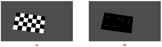
Figure 8.
Example synthetic images of the checkerboard (a) and the bead array (b) targets, at the same relative position.
3.1.1. Evaluating the Performance of Marker Detection
The performance of the marker detection algorithm was evaluated by comparing the ground truth and detected feature center points for each of the 20 images of the main synthetic dataset, as shown in Figure 9. The difference in image coordinates between the detected and ground truth points is shown in Figure 10 in the x and y dimensions. This representation shows that error in feature detection is well in the sub-pixel range for the studied range of positions. For comparison, results of the gold-standard algorithm for checkerboard detection with sub-pixel refinement of [] are included.
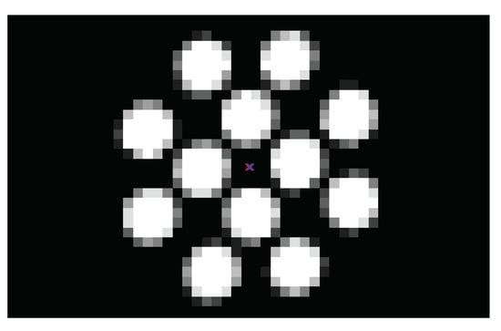
Figure 9.
Cropped section of a synthetic image of the bead array target. The center of the marker detected from the image is shown in red, while the ground truth value is shown in blue.
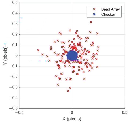
Figure 10.
Error in the X and Y axes corresponding to the detection of marker centroids (x) and checkerboard corners (*) in synthetic data. Each data point represents an image feature point.
3.1.2. Evaluating the Performance of Pose Estimation
Performance of position determination was evaluated by comparing the calculated reference-camera-to-target transformations () to the ground truth. We calculate the translation error () between the estimated and ground truth rigid body transformations as the Euclidean distance in each of the two axes that are parallel to the target plane. Since it is not relevant for the alignment task, we disregard the depth axis.
The rotation error () is calculated as the absolute difference between the magnitude of the angle around the rotation axis (as defined in the axis-angle representation). At this stage, we use the ground truth feature point coordinate values. We evaluate the performance of monocular and stereoscopic estimates for baseline values of 100, 150, 200, 250, and 300 mm. We observed that using ground truth feature points, errors are in the range of mm in translation and degrees in rotation for all approaches, which is considered to be insignificant. Therefore, in the following experiments, random noise with a uniform distribution and several range values was added to the feature point coordinate values, and the results were averaged over 20 tests.
In Figure 11, we present position estimation errors and , averaged over the 20 positions of the synthetic dataset for added noise in the range of −0.5 to 0.5 pixels. We can see that stereoscopic estimation produces the best results and performs better as the baseline increases. We can also see that standard deviation follows the same trend, showing that more consistent results are found with stereo, particularly for higher baseline values.
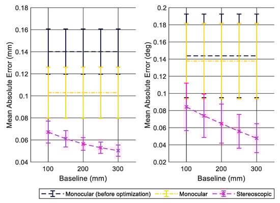
Figure 11.
Translation (left side) and rotation (right side) error of position estimation over the images of the synthetic dataset using ground truth feature points with added random noise within the interval of [−0.5, 0.5] pixels. Data points in the graph represent the average error over the 20 images of the dataset and error bars represent the standard deviation.
In Figure 12, we compare the performance of monocular and stereoscopic approaches for the smallest and largest considered baselines as a function of the added noise level. We see that stereoscopic estimation performs best and is the most robust to added noise. We observe that the error for approaches using stereo vision becomes lower as the cameras’ baseline increases for all considered noise levels.
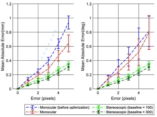
Figure 12.
Translation (left side) and rotation (right side) error of position estimation over the images of the synthetic dataset using ground truth feature points for several added noise levels. Data points in the graph represent the average error over the 20 images of the dataset and error bars represent the standard deviation.
We can consider in the application a baseline range of 100–300 mm and a maximum expected corner noise level of two pixels. In these conditions, the difference in translation and rotation error between monocular and stereoscopic estimates is less than 0.1 mm and 0.1 degrees.
3.2. Real Data
3.2.1. Experimental Setup
Our experimental setup is shown in Figure 13. The KUKA KR 16 L6-2 industrial robot was used to simulate the manipulator that would be used in the application. The manufacturing of the entire target assembly, as described in the methods section, is costly and time-consuming; therefore, it was approximated by a prototype of similar characteristics. The glass beads are made of borosilicate glass (n = 1.48) instead of fused silica (n = 1.46) and the sieve-like holding structure is made of a single 1 mm thick metal piece attached to a prototype of the target.
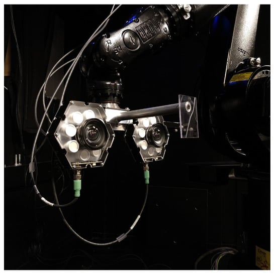
Figure 13.
Experimental setup.
We use two Basler acA1920-50gc industrial machine vision cameras with native resolution of 1920 × 1200. The cameras have an RGB Bayer filter to produce color images. To emulate the use of radiation-tolerant (RADTOL) cameras, the images were converted to grayscale in-camera. The original resolution was down-sampled by a factor of three using a bicubic kernel on 4 × 4 neighborhoods. The resulting effective resolution (640 × 400) is close to that of a RADTOL camera that we considered as a reference, the Visatec RC2 (586 × 330), producing a fairly realistic approximation of the image quality of the application. We used lenses with 6 mm focal length that had a horizontal field of view of approximately 82 degrees. The stereo camera pair was attached to a metal plate and had a fixed baseline of 210 mm. A set of radial illuminators (Smart Vision RC130) were mounted as closely as possible to the camera lenses. Each illuminator was constituted of eight high-intensity LEDs that create a near collimated, uniform light pattern that has a diameter of 280 mm at a distance of 500 mm from the lamp. In Figure 14, we show an example image taken in these conditions. For calibration of the cameras, we used a set of 20 images of a 24 × 17 checkerboard pattern.
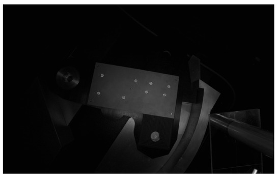
Figure 14.
Example image. The bead arrays can be seen as significantly brighter spots in an otherwise underexposed background.
3.2.2. Reference Values
The reference values for assessing the accuracy of the system were obtained by using an alignment piece, shown in Figure 15, made of a transparent polymer that had been engraved with alignment axes. Reference values were obtained by manually positioning the alignment piece in the aligned position and acquiring the transformation provided by the manipulator’s CS, .
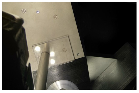
Figure 15.
Image of part of the target and the developed alignment piece in the aligned position.
Provided that the robot’s TCP has been assigned to the cross-hair, the transformation between the TCP and the target origin is, in the aligned position, the identity matrix. The definition of the TCP position is a built-in function of the KUKA robot controller, where the transformation between the robot’s flange and the alignment piece is estimated through the XYZ Four-Point TCP Calibration Method. This method involves bringing the tool center to a known position and recording several points as the position is approached from different orientations.
For a given test position, i, the rigid body transformation between the optical axis of the camera and the coordinate system of the target, , is given as follows:
where is provided by the robot’s CS at position i and is the calibrated hand–eye transformation. The transformation between the tool center point, , is the identity matrix. In our experiments, for each test position, we estimate and compare it with the reference value described above.
3.2.3. Evaluation of Overall System Performance
The overall performance of the proposed system is evaluated in a set of 20 initial camera positions, similar to those described in Section 3.1. In Figure 16, we show the translation errors between the estimated and ground truth transformations in each of the two axes that are parallel to the target plane.
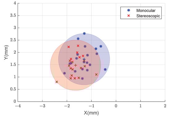
Figure 16.
Error in each of the X and Y axes for monocular (blue) and stereoscopic (red) estimates using our proposed approach.
3.2.4. Evaluation of Position Estimation
The performance of the position determination step was evaluated by using a checkerboard pattern as a target and full-resolution images. We used a state-of-the-art checkerboard detection algorithm [], which is considered to be very accurate. In this manner, we attempted to limit, to the extent possible, the effect of the developed target and marker detection methods on the results.
This experiment was run on approximately the same camera poses as described above. The distance between the camera and the target was increased to fit the larger checkerboard target in the cameras’ fields of view. The results are presented in Figure 17.
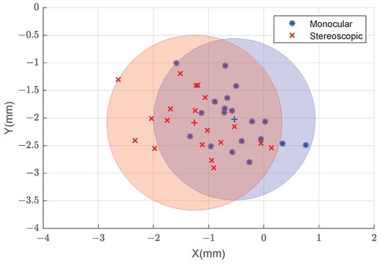
Figure 17.
Error in each of the X and Y axes for monocular (blue) and stereoscopic (red) estimates using corner values provided by the checkerboard detection algorithm in full-resolution images.
3.2.5. Study of the Effect of Camera Slant in the Original Position on the Overall System Performance
For the sake of completeness, an extensive analysis was conducted over a more comprehensive set of positions outside of the limits established in Section 3.1. We analyzed a set of 296 images taken at random initial camera positions and orientations.
In Figure 18, Figure 19 and Figure 20, we present the results as a function of the characteristics of the initial position: total rotation between camera and target and the horizontal and vertical deviation (Euclidean distance) from the central position and distance between the camera and the target. In these figures, the red cross signifies the mean of the observations and the dashed black circle represents the error tolerance of the application.
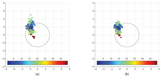
Figure 18.
Error in each of the X and Y axis for the estimation provided by the monocular (a) and stereoscopic (b) approaches. The colours represent the total rotation between the camera and target planes.
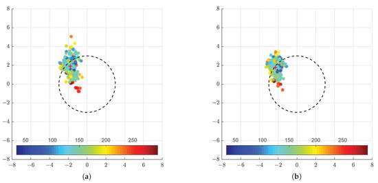
Figure 19.
Error in each of the X and Y axis for the estimation provided by the monocular (a) and stereoscopic (b) approaches. The colours represent the horizontal and vertical deviation from the from the central position.
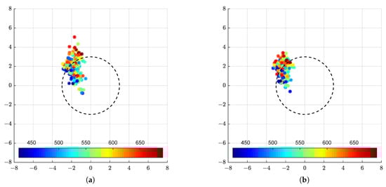
Figure 20.
Error in each of the X and Y axis for the estimation provided by the monocular (a) and stereoscopic (b) approaches. The colours represent the distance between the camera and target.
3.2.6. Comparison to the Earlier Solution
In order to establish a comparison between the newly developed marker-based method and the approach of [], we ran corresponding data through their method that consists of estimating a 3D representation of the scene by stereo matching and aligning it to the reference CAD model using an iterative closest point (ICP) algorithm. To obtain corresponding data, we captured the same sequence of robot poses with the same scene object, but with different lighting conditions. Since the stereo reconstruction relies on Lambertian reflectivity of the target object, it requires more light than the new marker-based approach.
The earlier approach relies on a number of parameters, which should be tuned to the current scene properties. This is needed to avoid falling into local minima and converging on false position estimates. To avoid the time-consuming manual tuning step to adapt to this particular setup, we gave an initial estimate to the algorithm based on the known true target position with an added offset. For the objective of measuring the accuracy (not the robustness) of the earlier solutions, this approach is justified for the sake of a comparison. We found that adding up to 25 mm of position error and five degrees of angular error still results in the algorithm converging as close to the correct position as the data allow (Figure 21, left side). Larger amounts (such as 50 mm and 10 degrees) make it difficult for ICP to find the correct neighborhood to converge, and the pose estimates start having large amounts of outliers (Figure 21, right side).
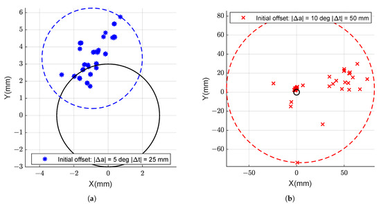
Figure 21.
Error in each of the X and Y axis for the estimation provided by the stereo ICP based method from earlier work, with different amounts of initial position deviation from ground truth. Offset values of |Δa| = 5 deg, |Δt| = 25 mm (a). Offset values of |Δa| = 10 deg, |Δt| = 50 mm (b). Each colour point represents a different position of the camera in relation to the target. The continuous black circle represents the error tolerance of the application.
3.2.7. Analyses of Overall System Performance Using an Image-Based Metric
An alternative, image-based metric was designed to evaluate the overall performance of the system without relying on the manual alignment procedure and alignment tool calibration (described in Section 3.2.2) to provide a reference value, allowing us to rule out errors in those processes. However, this metric expresses not only the accuracy of our system and the ability of the robot’s CS to report its position correctly, but also its ability to reach the target position. Therefore, we can expect the overall errors to be potentially higher.
The procedure starts by capturing an image at the initial position and calculating the transformation between the left camera and the target, , using our developed methods. As a second step, the base-to-end-effector transformation that brings the camera to the desired position, , is determined by:
where , the transformation between the camera and the target in the desired position, has the value:
which corresponds to aligning the camera and target plane at a distance of 250 mm from the target. The command is given to the robot controller, which moves the camera to the calculated position, where a full-resolution image of the target is taken (Figure 22).
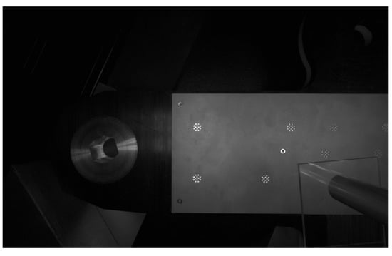
Figure 22.
Example image taken at the aligned position. If the estimate is correct, the center of the reference marker should correspond to the center of the image.
If the alignment is correct, the center of the reference marker is expected to coincide with the center of the image. Therefore, an alignment error can be measured in pixels, i.e., as the difference between the center of the marker and the center of the image (Figure 23). The measured error can be converted into millimeters, since the dimensions of the target are known (e.g., we know that the diameter of one bead corresponds to 1.95 mm).
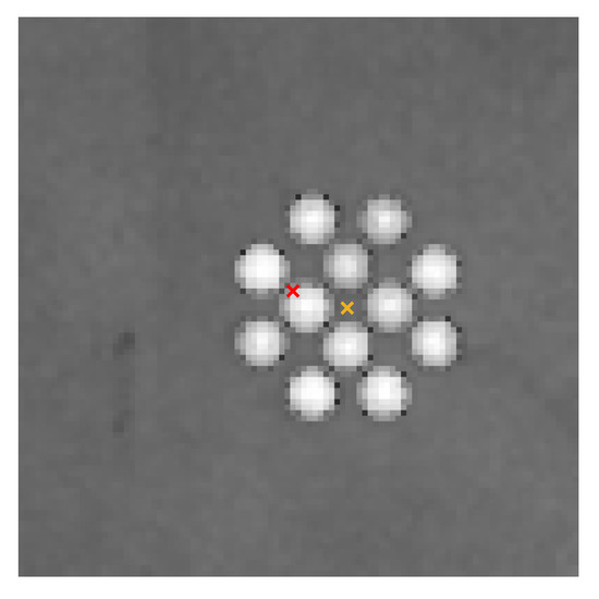
Figure 23.
Example of a cropped image taken at the aligned position. The yellow cross represents the center of the marker and the red cross the center of the image. A combined overall performance error can be calculated, in pixels, as the difference between the two points.
In Figure 24, we show the calculated error using this method for the set of 20 initial camera positions that we have been analyzing so far.
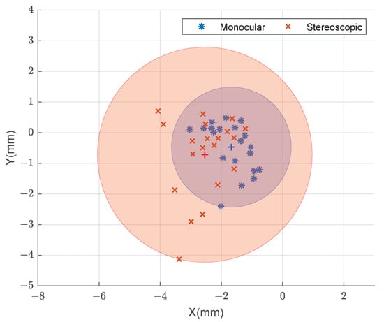
Figure 24.
Error in each of the X and Y axes for monocular (blue) and stereoscopic (red) estimates provided by the image-based method.
3.2.8. Discussion
Through the study of the overall performance of the system, we conclude that both the monocular and stereoscopic approaches satisfy the requirements of the application for the studied range of positions, as all data points are within the ±3 mm tolerance (Figure 16). Furthermore, the results are considered to be quite precise, as the errors are distributed within a circle of approximately 1 mm radius around the mean value. There are no significant performance differences between the monocular and stereoscopic approaches. This indicates that the system can be simplified to its monocular version without significant loss of accuracy or precision. This is a clear improvement over methods based on 3D reconstruction from multiple cameras, since the physical space on the manipulator is limited.
When using the reference method for marker detection (checkerboard target), we observe a similar trend in the results (Figure 17). However, precision is lower, with errors distributed in a circle of around 1.5 mm radius around the mean value, which is likely related with the increased distance between the camera and the target.
In all experiments, regardless of the evaluation metric, we observe an offset in the estimated errors. When relating the local coordinate systems of the targets with the physical setup, it becomes clear that the offset has a strong directional component that coincides with the gravity vector. Furthermore, the remaining directional components of the offset tend to follow the direction in which the end effector extends from the base. The offset can be traced back to an error in the positions reported by the control system of the robot, and it is higher the further the arm extends from the robot base. This data leads us to conclude that the offset is related to a deflection of the robot base under the manipulator’s weight.
This is a known problem in robotics, often tackled through non-kinematic calibration of the manipulator. Non-kinematic calibration of robot manipulators is of particular interest to the ITER application due to the fact that the high payloads can cause considerable deflections of the robot base []. However, the investigation of such methods falls out of the scope of this work, and in our results, no methods have been applied to compensate for this deviation.
Therefore, in the upcoming discussion on how several characteristics of the initial pose affect the quality of our estimate, we consider better estimates those that are nearest the mean error value.
In this setting, it is clear from Figure 18 that the overall system provides better estimates for less slanted initial camera positions. This is likely influenced by the characteristics of the developed marker detection algorithm, which assumes that the centroid of the detected ellipses in the images corresponds to the center of the circular markers. This approximation is better when the camera plane and the object plane are parallel. We also note that the stereoscopic estimation seems to have a more advantageous performance for higher angles, reducing the spread of the results and increasing the precision of our estimation.
In Figure 19, we see that a higher distance from the central position is similarly associated with worst estimates, although the difference is not as obvious as in the previous case.
As Figure 18 and Figure 19 indicate, images from initial poses with lower angle and smaller distance generally lead to consistent estimates closest to the mean error, i.e., have the best precision. In Figure 20, we see a slightly different pattern. Higher distance from the target is associated with higher error, while poses closer to the target have error closer to 0. We can conclude that there is a direct influence of the distance to the target (and degree to which the robot arm is extended) on the reported error values.
As the comparison between Figure 16 and Figure 21 shows, our proposed approach significantly outperforms, as hypothesized, the state-of-the-art method for pose estimation in the ITER environment, even while using a single camera. Furthermore, our approach is significantly more tolerant to the variation of light conditions, needing far less fine-tuning to be adapted to a new setting. The maximum deviation from the mean is, in the best case, around 3 mm, contrasting with the 1 mm of the proposed approach and consuming all the available tolerance.
The experiment that uses an image-based metric (Figure 24) provides a similar distribution of error to those of the other experiments, although both the precision and accuracy are lower due to the inclusion of the alignment task.
4. Conclusions
Our studies demonstrate that marker-based tracking is a suitable option for localization of the elements of the divertor remote handling system of the ITER, as well as for other similar applications. Even though characteristics of these environments might invalidate the use of retro-reflective markers of the kind conventionally used in photogrammetry, such as retro-reflective tape, we have shown that it is possible to develop a custom made retro-reflective marker out of materials that are commonly used in industrial environments (stainless steel and fused silica). The results of the overall system performance are within the targeted range of error and the system was demonstrated to work quite robustly, even without compensating for the deviations in the positions reported by the manipulator’s control system. Furthermore, the proposed approach was demonstrated to be considerably better than the earlier stereo-matching-based solution. It was demonstrated that the system can be simplified to a single camera without significant loss of accuracy or precision.
Further developments of this work should include the optimization of the brilliancy of the retro-reflective markers, as well as the development of marker detection and correspondence methods to allow handling of marker occlusion. Further, it is particularly relevant that future studies consider how the errors caused by the deflection of the robot base under the manipulator’s weight can be estimated and compensated, taking into account the high and variable payloads in the ITER application. How the information computed by the proposed system can be optimally presented to the operator and the effect of the availability of this information on teleoperation performance should also be subject to a dedicated study in the future.
Author Contributions
Conceptualization, L.G.R. and O.J.S.; Methodology, L.G.R. and O.J.S.; Project administration, O.J.S. and E.R.M.; Resources, A.D.; Software, L.G.R.; Supervision, O.J.S., S.P., and A.G.; Validation, L.G.R.; Writing—original draft, L.G.R.; Writing—review and editing, O.J.S., S.P., and A.G. All authors have read and agreed to the published version of the manuscript.
Funding
The work in this paper was funded by the European Union’s Horizon 2020 research and innovation program under the Marie Sklodowska Curie grant agreement No. 764951, Immersive Visual Technologies for Safety-Critical Applications and by Fusion for Energy (F4E), and Tampere University under the F4E grant contract F4E-GRT-0901. This publication reflects the views only of the authors, and Fusion for Energy cannot be held responsible for any use which may be made of the information contained herein. The research infrastructure of the Center for Immersive Visual Technologies (CIVIT) at Tampere University provided the robotic manipulator, sensors, and laboratory space for conducting the experiments.
Conflicts of Interest
The authors declare no conflict of interest. This publication reflects the views only of the authors, and Fusion for Energy cannot be held responsible for any use which may be made of the information contained herein.
References
- Pérez, L.; Rodríguez, Í.; Rodríguez, N.; Usamentiaga, R.; García, D.F. Robot guidance using machine vision techniques in industrial environments: A comparative review. Sensors 2016, 16, 335. [Google Scholar] [CrossRef] [PubMed]
- Malamas, E.N.; Petrakis, E.G.; Zervakis, M.; Petit, L.; Legat, J.D. A survey on industrial vision systems, applications and tools. Image Vis. Comput. 2003, 21, 171–188. [Google Scholar] [CrossRef]
- Lichiardopol, S. A Survey on Teleoperation; DCT Rapporten; Vol. 2007.155; Technical Report; Technische Universiteit Eindhoven: Eindhoven, The Netherlands, 2007. [Google Scholar]
- Hoff, W.A.; Gatrell, L.B.; Spofford, J.R. Machine vision based teleoperation aid. Telemat. Inform. 1991, 4, 403–423. [Google Scholar] [CrossRef][Green Version]
- Miyanishi, Y.; Sahin, E.; Makinen, J.; Akpinar, U.; Suominen, O.; Gotchev, A. Subjective comparison of monocular and stereoscopic vision in teleoperation of a robot arm manipulator. Electron. Imaging 2019, 2019, 659-1–659-6. [Google Scholar] [CrossRef]
- Tesini, A.; Palmer, J. The ITER remote maintenance system. Fusion Eng. Des. 2008, 83, 810–816. [Google Scholar] [CrossRef]
- Sanders, S.; Rolfe, A. The use of virtual reality for preparation and implementation of JET remote handling operations. Fusion Eng. Des. 2003, 69, 157–161. [Google Scholar] [CrossRef]
- Heemskerk, C.; De Baar, M.; Boessenkool, H.; Graafland, B.; Haye, M.; Koning, J.; Vahedi, M.; Visser, M. Extending Virtual Reality simulation of ITER maintenance operations with dynamic effects. Fusion Eng. Des. 2011, 86, 2082–2086. [Google Scholar] [CrossRef]
- Niu, L.; Aha, L.; Mattila, J.; Gotchev, A.; Ruiz, E. A stereoscopic eye-in-hand vision system for remote handling in ITER. Fusion Eng. Des. 2019. [Google Scholar] [CrossRef]
- Niu, L.; Smirnov, S.; Mattila, J.; Gotchev, A.; Ruiz, E. Robust pose estimation with the stereoscopic camera in harsh environment. Electron. Imaging 2018, 1–6. [Google Scholar] [CrossRef]
- Burgess, G.; Shortis, M.; Scott, P. Photographic assessment of retroreflective film properties. ISPRS J. Photogramm. Remote Sens. 2011, 66, 743–750. [Google Scholar] [CrossRef]
- Schauer, D.; Krueger, T.; Lueth, T. Development of autoclavable reflective optical markers for navigation based surgery. In Perspective in Image-Guided Surgery; World Scientific: Singapore, 2004; pp. 109–117. [Google Scholar] [CrossRef]
- Bhatnagar, D.K. Position Trackers for Head Mounted Display Systems: A Survey; University of North Carolina: Chapel Hill, NC, USA, 1993; Volume 10. [Google Scholar]
- Vogt, S.; Khamene, A.; Sauer, F.; Niemann, H. Single camera tracking of marker clusters: Multiparameter cluster optimization and experimental verification. In Proceedings of the International Symposium on Mixed and Augmented Reality, Darmstadt, Germany, 1 October 2002; pp. 127–136. [Google Scholar] [CrossRef]
- Bergamasco, F.; Albarelli, A.; Torsello, A. Pi-tag: A fast image-space marker design based on projective invariants. Mach. Vis. Appl. 2013, 24, 1295–1310. [Google Scholar] [CrossRef]
- Nakazato, Y.; Kanbara, M.; Yokoya, N. Localization of wearable users using invisible retro-reflective markers and an IR camera. In Proceedings of the Stereoscopic Displays and Virtual Reality Systems XII, International Society for Optics and Photonics, San Jose, CA, USA, 22 March 2005; Volume 5664, pp. 563–570. [Google Scholar]
- Sereewattana, M.; Ruchanurucks, M.; Siddhichai, S. Depth estimation of markers for UAV automatic landing control using stereo vision with a single camera. In Proceedings of the International Conference Information and Communication Technology for Embedded System, Ayutthaya, Thailand, 23–25 January 2014. [Google Scholar]
- Faessler, M.; Mueggler, E.; Schwabe, K.; Scaramuzza, D. A monocular pose estimation system based on infrared leds. In Proceedings of the 2014 IEEE International Conference on Robotics and Automation (ICRA), Hong Kong, China, 31 May–5 June 2014; pp. 907–913. [Google Scholar] [CrossRef]
- Hattori, S.; Akimoto, K.; Fraser, C.; Imoto, H. Automated procedures with coded targets in industrial vision metrology. Photogramm. Eng. Remote Sens. 2002, 68, 441–446. [Google Scholar]
- Tushev, S.; Sukhovilov, B.; Sartasov, E. Architecture of industrial close-range photogrammetric system with multi-functional coded targets. In Proceedings of the 2017 2nd International Ural Conference on Measurements (UralCon), Chelyabinsk, Russia, 16–19 October 2017; pp. 435–442. [Google Scholar] [CrossRef]
- San Biagio, M.; Beltran-Gonzalez, C.; Giunta, S.; Del Bue, A.; Murino, V. Automatic inspection of aeronautic components. Mach. Vis. Appl. 2017, 28, 591–605. [Google Scholar] [CrossRef]
- Liu, T.; Burner, A.W.; Jones, T.W.; Barrows, D.A. Photogrammetric techniques for aerospace applications. Prog. Aerosp. Sci. 2012, 54, 1–58. [Google Scholar] [CrossRef]
- Clarke, T.A. Analysis of the properties of targets used in digital close-range photogrammetric measurement. In Proceedings of the Videometrics III, International Society for Optics and Photonics, Boston, MA, USA, 6 October 1994; Volume 2350, pp. 251–262. [Google Scholar] [CrossRef]
- Dong, M.; Xu, L.; Wang, J.; Sun, P.; Zhu, L. Variable-weighted grayscale centroiding and accuracy evaluating. Adv. Mech. Eng. 2013, 5, 428608. [Google Scholar] [CrossRef]
- Bender, P.; Wilkinson, D.; Alley, C.; Currie, D.; Faller, J.; Mulholland, J.; Siverberg, E.; Plotkin, H.; Kaula, W.; MacDonald, G. The Lunar laser ranging experiment. Science 1973, 182, 229–238. [Google Scholar] [CrossRef]
- Feng, Q.; Zhang, B.; Kuang, C. A straightness measurement system using a single-mode fiber-coupled laser module. Opt. Laser Technol. 2004, 36, 279–283. [Google Scholar] [CrossRef]
- Nakamura, O.; Goto, M.; Toyoda, K.; Takai, N.; Kurosawa, T.; Nakamata, T. A laser tracking robot-performance calibration system using ball-seated bearing mechanisms and a spherically shaped cat’s-eye retroreflector. Rev. Sci. Instrum. 1994, 65, 1006–1011. [Google Scholar] [CrossRef]
- Shortis, M.R.; Seager, J.W. A practical target recognition system for close range photogrammetry. Photogramm. Rec. 2014, 29, 337–355. [Google Scholar] [CrossRef]
- Ribeiro, L.G.; Suominen, O.; Peltonen, S.; Morales, E.R.; Gotchev, A. Robust Vision Using Retro Reflective Markers for Remote Handling in ITER. Fusion Eng. Des. 2020, 161, 112080. [Google Scholar] [CrossRef]
- Lundvall, A.; Nikolajeff, F.; Lindström, T. High performing micromachined retroreflector. Opt. Express 2003, 11, 2459–2473. [Google Scholar] [CrossRef] [PubMed]
- Stoudt, M.; Vedam, K. Retroreflection from spherical glass beads in highway pavement markings. 1: Specular reflection. Appl. Opt. 1978, 17, 1855–1858. [Google Scholar] [CrossRef] [PubMed]
- Yuan, J.; Chang, S.; Li, S.; Zhang, Y. Design and fabrication of micro-cube-corner array retro-reflectors. Opt. Commun. 2002, 209, 75–83. [Google Scholar] [CrossRef]
- Shin, S.Y.; Lee, J.I.; Chung, W.J.; Cho, S.H.; Choi, Y.G. Assessing the refractive index of glass beads for use in road-marking applications via retroreflectance measurement. Curr. Opt. Photonics 2019, 3, 415–422. [Google Scholar] [CrossRef]
- Yongbing, L.; Guoxiong, Z.; Zhen, L. An improved cat’s-eye retroreflector used in a laser tracking interferometer system. Meas. Sci. Technol. 2003, 14, N36. [Google Scholar] [CrossRef]
- MATLAB. Version 9.6.0 (R2019a); The MathWorks Inc.: Natick, MA, USA, 2019. [Google Scholar]
- Zhang, Z. A flexible new technique for camera calibration. IEEE Trans. Pattern Anal. Mach. Intell. 2000, 22, 1330–1334. [Google Scholar] [CrossRef]
- Heikkila, J.; Silven, O. A four-step camera calibration procedure with implicit image correction. In Proceedings of the IEEE Computer Society Conference on Computer Vision and Pattern Recognition, San Juan, Puerto Rico, 17–19 June 1997; pp. 1106–1112. [Google Scholar] [CrossRef]
- Tan, L.; Wang, Y.; Yu, H.; Zhu, J. Automatic camera calibration using active displays of a virtual pattern. Sensors 2017, 17, 685. [Google Scholar] [CrossRef]
- Ali, I.; Suominen, O.; Gotchev, A.; Morales, E.R. Methods for Simultaneous Robot-World-Hand–Eye Calibration: A Comparative Study. Sensors 2019, 19, 2837. [Google Scholar] [CrossRef]
- Bradley, D.; Roth, G. Adaptive thresholding using the integral image. J. Graph. Tools 2007, 12, 13–21. [Google Scholar] [CrossRef]
- Soille, P. Morphological Image Analysis: Principles and Applications; Springer Science & Business Media: Berlin/Heidelberg, Germany, 2013. [Google Scholar] [CrossRef]
- Haralick, R.M.; Shapiro, L.G. Computer and Robot Vision; Addison-Wesley: Boston, MA, USA, 1992; Volume 1, pp. 28–48. [Google Scholar]
- Ahn, S.J.; Rauh, W.; Kim, S.I. Circular coded target for automation of optical 3D-measurement and camera calibration. Int. J. Pattern Recognit. Artif. Intell. 2001, 15, 905–919. [Google Scholar] [CrossRef]
- Mallon, J.; Whelan, P.F. Which pattern? Biasing aspects of planar calibration patterns and detection methods. Pattern Recognit. Lett. 2007, 28, 921–930. [Google Scholar] [CrossRef]
- Collins, T.; Bartoli, A. Infinitesimal plane-based pose estimation. Int. J. Comput. Vis. 2014, 109, 252–286. [Google Scholar] [CrossRef]
- Schweighofer, G.; Pinz, A. Robust pose estimation from a planar target. IEEE Trans. Pattern Anal. Mach. Intell. 2006, 28, 2024–2030. [Google Scholar] [CrossRef] [PubMed]
- Sturm, P. Algorithms for plane-based pose estimation. In Proceedings of the IEEE Conference on Computer Vision and Pattern Recognition, CVPR 2000 (Cat. No. PR00662), Hilton Head Island, SC, USA, 13–15 June 2000; Volume 1, pp. 706–711. [Google Scholar] [CrossRef]
- Hartley, R.; Zisserman, A. Multiple View Geometry in Computer Vision; Cambridge University Press: Cambridge, MA, USA, 2003. [Google Scholar] [CrossRef]
- Levenberg, K. A method for the solution of certain non-linear problems in least squares. Q. Appl. Math. 1944, 2, 164–168. [Google Scholar] [CrossRef]
- Marquardt, D.W. An algorithm for least-squares estimation of nonlinear parameters. J. Soc. Ind. Appl. Math. 1963, 11, 431–441. [Google Scholar] [CrossRef]
- Rodriguez, O. Des lois geometriques qui regissent les desplacements d’un systeme solide dans l’espace et de la variation des coordonnees provenant de deplacements consideres independamment des causes qui peuvent les produire. J. Math. Pures Appl. 1840, 5, 380–440. [Google Scholar]
- Geiger, A.; Moosmann, F.; Car, Ö.; Schuster, B. Automatic camera and range sensor calibration using a single shot. In Proceedings of the 2012 IEEE International Conference on Robotics and Automation, Saint Paul, MN, USA, 14–18 May 2012; pp. 3936–3943. [Google Scholar] [CrossRef]
- Kivelä, T.; Saarinen, H.; Mattila, J.; Hämäläinen, V.; Siuko, M.; Semeraro, L. Calibration and compensation of deflections and compliances in remote handling equipment configurations. Fusion Eng. Des. 2011, 86, 2043–2046. [Google Scholar] [CrossRef]
Publisher’s Note: MDPI stays neutral with regard to jurisdictional claims in published maps and institutional affiliations. |
© 2020 by the authors. Licensee MDPI, Basel, Switzerland. This article is an open access article distributed under the terms and conditions of the Creative Commons Attribution (CC BY) license (http://creativecommons.org/licenses/by/4.0/).