Build Orientation Optimization Based on Weighted Analysis of Local Surface Region Curvature

Abstract

Build orientation becomes a hot issue in 3D printing, which has a significant impact on the surface quality, support structure and final cost of the fabricated model. In this paper, we focus our attention on the surface quality of the part when fabricated by a 3D printer under certain specific build orientation. A novel method using curvature shift is proposed to search local regions with obvious curvature changes of the model printed. Based on curvature shift strategy, the model is divided into separate regions which can be treated differently. Every triangle facet of the regions is given different weight factor by calculating the average curvature of each region. Weighted facets is introduced in building volume error function. Candidate build orientation can be obtained by the eigenvalue decomposition and the optimal build orientation is the one which leads to the minimal error of the function. From the case study, the method proposed gets a smaller error with a lower printing cost and time, which means the model surface in higher weighted regions gets a higher surface quality when printed.

1. Introduction

3D printing or additive manufacturing (AM, rapid prototyping, layer manufacturing, free-form fabrication, rapid manufacturing) is a process where parts are manufactured according to a digital 3D model by adding material, usually layer by layer along the build orientation, as opposed to subtractive manufacturing methodologies such as traditional milling [1]. The original CAD model of the fabricated part can be designed by commercial CAD software or reconstructed via reverse engineering. Once the CAD model is available, layer slice program is applied to deal with the model and output all the 2-D contour layers, then 3D printers print the model layer by layer. The build orientation needs to be determined first before printing. Only when the build orientation is already known can we set the other necessary printing parameters, slice the model and print it by 3D printing.

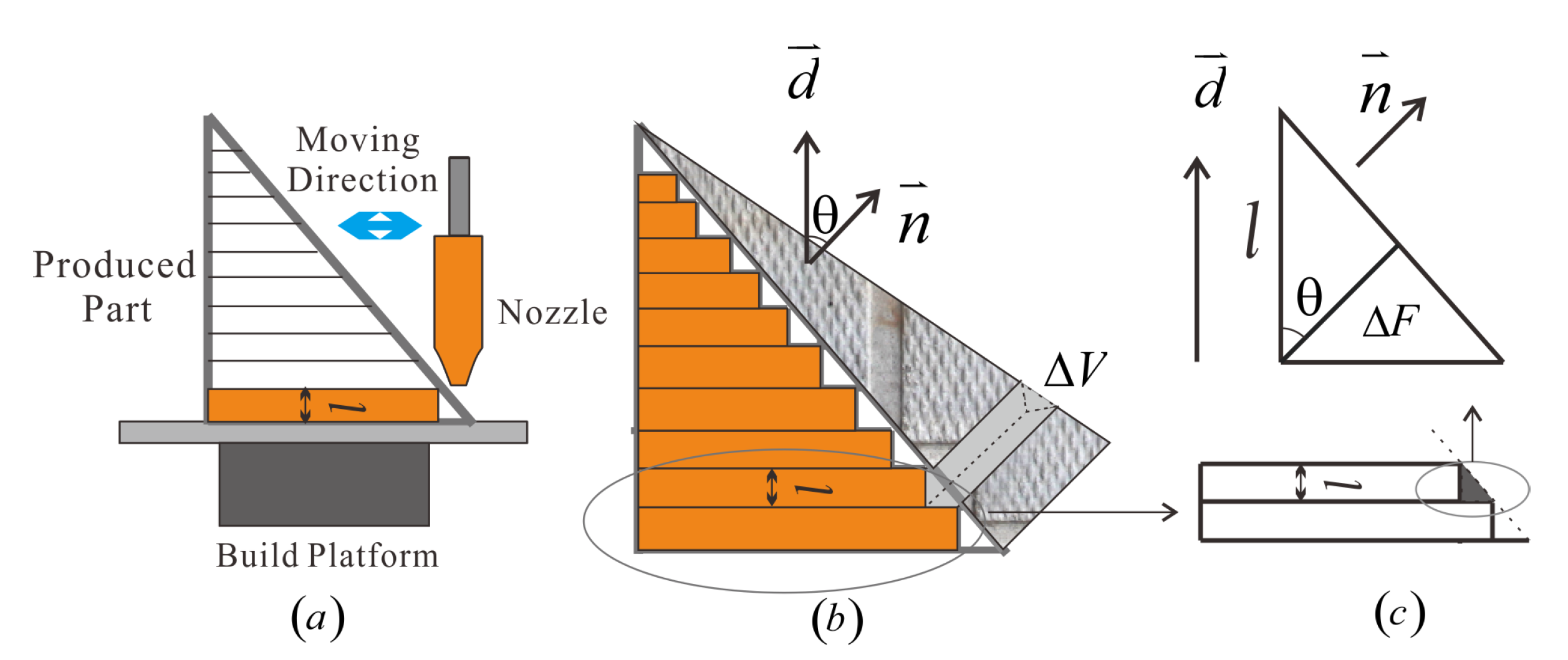
We all know that the inherent defect of 3D printing technique: the staircase effect [2,3,4] occurs in the process of layer by layer addition shown in Figure 1a. If the nozzle size is smaller and the layer thickness is thinner, the surface quality can be greatly improved, however it takes a long time to fabricate. It is actually a contradiction between efficiency and surface quality. When the hardware parameters of the 3D printer are determined, the build orientation has a great influence on the surface accuracy caused by the staircase error. Therefore, this paper will focus on reducing the staircase error in the pre-processing of 3D printing models. As for the effect of printing, process parameters and material shaping on the surface accuracy of the model are not involved.

If the build orientation is parallel or vertical to the surface facet of the model printed, the staircase effect disappears. If the angle $\theta$ (shown in Figure 1b) between the surface normal $\overrightarrow{n}$ and the build orientation $\overrightarrow{d}$ is between 0 and 90 degrees, the staircase effect occurs and the surface quality decreases. The build orientation determines surface quality of the part and even its mechanical properties [5]. However, for most part models, the normal direction of the surface is rarely perpendicular or parallel to the build orientation, and the staircase error is unavoidable. Therefore, it is very necessary to improve the accuracy of certain regions of the printed part by adjusting the build orientation [6]. Based on the principle of generation, we add the regional weight to the staircase error function, and obtain the candidate build orientation through eigenvalue decomposition to improve the surface quality of the region. The objective of this article was to find local regions with obvious curvature changes in the surface of the printed part from a geometric point of view, which is then given a high weight factor. Of course, according to the different application scenarios and performance of the fabricated part, different regions of the part require different surface quality. However, this article does not consider this problem.

In this paper, a novel optimization of part build orientation based on weighted analysis of local surface region curvature is proposed. The rest of this paper is structured as follows: Section 2 presents the related studies of the optimization of build orientation. Section 3 presents a detailed explanation of the methodology based on the curvature shift process. This is followed by case study on test models in Section 4. Finally, the conclusions and future scope of this work are presented in Section 5.

2. Literature Review

Due to the importance of build orientation in AM, intensive researches are conducted to provide feasible solutions. An attempt is made to achieve minimum average part surface roughness (best overall surface quality), minimum build time and support structure for stereo lithography (SL) and selective laser sintering (SLS) processed parts by determining optimum part build orientation [7,8,9,10]. For most simple models, the direction parallel to a coordinate axis is used as the build orientation [11]. It cannot be the same as complicated models. Most researchers usually chooses single or multiple factors to construct a single-object or multi-object optimization function and find the best build orientation from the feasible solution by determining the weight and range for the optimization target [12,13,14,15,16,17,18,19,20,21].

On the research of a single target method, most researchers take one factor such as volume deviation or surface roughness to build the object function, which can get the optimal build orientation under the specific factor chosen [12,13,14,15,16,17]. Ahar et al. [12] determines the optimal build orientation based on the position of normal vectors of the original CAD model. All the normal vectors are considered as the candidate orientation. It is certainly feasible to adopt an exhaustive approach, but subject to the existing surface normals. It is difficult to get the optimal build orientation. Luo et al. [13] used a new volume error model. The biggest problem is that all normal-weighted regions are weighted equally. The geometry features of the model itself are neglected and the weighted optimization process essentially belongs to normal weight, which means all facets contribute equally to the optimal build orientation. Ding et al. [14] proposed a new method to determine the optimal build orientation using Gauss Map, which collects all facet normals in a unit sphere. The unit vector from the center of the sphere to the center of the bottom circle of the spherical crown is the optimal build direction. Although just considering the facet normal, it effectively decreases the volume of support structure. It should be noted that the algorithm is not versatile especially for some more complex parts which contain open concave loops or non-sharp edges. Bruno et al. [15] researched the effect of different build orientations on Ti-6Al-4V for microstructural and mechanical property evaluation. However, printing performance is more affected by material properties and cooling deformation after thermoforming. Relatively speaking, the build orientation has relatively little influence. Barclift et al. [16] used particle swarm optimization [17] to search an optimal build orientation owing to its ease of programming, convergence speed and computational efficiency. If the initial particle is not good, it may be biased by a certain particle. The algorithm is easy to converge prematurely and fall into a local optimal solution. In addition, the complexity of the algorithm increases, resulting in reduced efficiency.

The multi-object method chooses multiple factors such as surface quality, construction time and material consumption to determine the optimal build orientation [18]. The proportion of each factor is determined empirically or based on the demand [19,20,21]. Phatak et al. [19] applied the genetic algorithm to solve the parameter optimization of multiple objects (staircase error, heights and materials cost). The method distributed different weight to the three factors and obtained the optimal orientation. A constrained non-linear multi-object optimization model is constructed based on the eight parameters [20]. The model is solved by global search algorithm in MatLAB. Different parameter weight is based on which parameter is more important. The results of the method show significant improvements in the manufactured part’s geometric accuracy and thus validate the performance of this approach. Brika et al. [21] proposed a multi-object optimization of surface roughness, build time and support structures. Utility function approach is adopted to convert the optimization problem into a linear-weighted function. The optimal build orientation is determined by iteratively inputting the parameter. Although the multi-objective optimization algorithm uses multiple research objects and assigns a certain weight to each object to select the optimal build orientation to ensure that the final printing effect meets the expected settings, there are common shortcomings. The requirements of each research object on the build orientation are different or even opposite, which leads to a contradictory calculation process in the orientation optimization process. If the weight of a research object is increased or decreased, in fact, the multi-objective optimization algorithm reduces the dimensionality to a single-objective optimization algorithm. It is back to the problem of single objective optimization.

With the rise of machine learning, machine learning (ML) has been applied in various aspects of 3D printing, such as design for 3D printing, material tuning, process optimization, in-situ monitoring, cloud serving and cybersecurity, to improve the whole design and manufacturing workflow especially in the era of industrial revolution 4.0 [22]. In recent years, many scholars have used machine learning to optimize 3D printing process parameters and part performance parameters, including the build orientation [23,24,25,26]. Malviya et al. [23] proposed a generalized machine learning-based parameter optimization framework to determine optimal build orientation for FDM(Fused Deposition Modeling) components. The mechanical properties of the test examples selected are tested and simulated from the three main directions of XYZ, and then the training data are obtained through orthogonal experiments. Obviously the algorithm does not have universal applicability and is not applicable to other complex models. The simulation data of complex models is definitely more than three main directions for testing. Zhang et al. [24] proposed a method that applies a non-supervised machine learning method, K-means clustering with DaviesBouldin criterion cluster measuring, to rapidly decompose a surface model into facet clusters and efficiently generate a set of meaningful alternative build orientations. Cluster analysis based on statistics takes a lot of time and it is difficult to converge for more complex models. CNNs is more precise at estimating all three studied factors than the baseline linear regression model for the training and evaluation conditions [25]. Machine learning algorithms have a great advantage for studying a class of models with similar characteristics. Given enough training data, it fits very well. When the model has anisotropic characteristics, either increase the training sample data or the new model needs to be re-learned to train the data. In addition, machine learning requires very high computer performance and it is more difficult to choose meta-parameters and network topology.

Build orientation impacts surface quality, build time, support volume and mechanical properties [27]. Despite that multi-object and heuristic-based optimization can be used to determine an orientation and lots of researchers focus their attention on multi-object optimization, it cannot solve collective effect of multi-factors synchronously to the optimization process. Once the weight of each factor is determined, it essentially degrades into simple object optimization. The only benefit that draws from multi-object optimization is we can easily obtain the balanced optimal result from the factors defined by giving the specific weight factor. In this paper, we only focus the effect of different build orientations on the surface quality of regions with higher curvature in the fabricated part.

3. Methodology

This section presents a detailed explanation of our method to implement the proposed optimization of build orientation. Firstly, a new method curvature shift is proposed to effectively classify the surface regions of the CAD model. The method divides the original model into different clusters and each cluster represents those points and facets that have similar geometry features. Secondly, the curvature of the point is defined and estimated based on the NURBS(Non-Uniform Rational B-Splines) surface reconstructed by the point as well as its 1-ring neighbor points. The point with the big curvature is distributed a big weight factor, which is determined by the number points of the CAD model and the different ratios of each point’s curvature. Thirdly, the volume error function with weight factor determined in the second step is built by calculating cusp height [28]. The orientation optimization is converted into a linear regression problem with the least absolute deviation. The least absolute deviation norm is appropriated by the least squares norm and PCA method to process eigenvalue decomposition on the scatter matrix of weighted norm vector. The optimal build orientation is finally determined from the eigenvectors which minimizes the volume error function.

3.1. Surface Region Analysis

Different regions of a part have different functions and the geometry accuracy has a great impact on the mechanic performance especially in the field of free-form surface [29]. By analyzing the surface region curvatures of the model, different regions of the model are assigned different weight factors, which can be used in the volume error function to calculate the optimal build orientation. To distribute a reasonable weight factor in different regions of the model, cluster strategy [30] is applied in the original model. The model is divided into several clusters and each cluster represents one set that has roughly similar features. Each cluster is considered as a separate module, which means the cluster appears interest points relative to other points instead of nearest neighbor search of the whole model such as thin tips and edges. Different regions are shown in different colors (Figure 2b) and each cluster is analyzed as a separate part in Section 3.2.

3.1.1. Cluster

Clustering algorithms are useful in information theory, target detection, communications, compression and other regions. There are mainly K-means clustering, hierarchical clustering, spectral clustering and mean shift clustering. K-means clustering is simple and efficient, but it is easily affected by the initial cluster center. Multiple hierarchical clustering has a large time complexity and the result of hierarchical clustering depends on the selection of the merging points and the splitting points of the clustering. Mean shift cluster searches for the cluster center along the direction of the increase in the highest density, which is not helpful to the recognize geometry features of the model. To solve this problem, curvature shift is proposed to classify the model into different clusters based on the geometry features. The weight factor is set for each cluster so that each point in the cluster has different importance to the vector of curvature shift (Section 3.1.3).

3.1.2. Curvature Estimation

The curvature shift method proposed mainly depends on the curvature of points. The curvature of one point on the model is defined as follows: the maximum curvature of the central point on the surface, which is reconstructed by the point with its 1-ring points. The maximum curvature reflects the changes in the polar region around the point. If the maximum curvature is close to zero, it shows that the polar region is relatively flat.

Surface reconstruction is used to estimate the curvature as shown in Figure 3. NURBS surface is adopted to the appropriate local sample. A NURBS surface is obtained as the tensor product of two NURBS curves, thus using two independent parameters u and v (with indices i and j, respectively) [21]:

$$S(u,v)=\sum _{i=1}^k\sum _{j=1}^l{R}_{i,j}(u,v)P_{i,j}$$

(1)

with

$$R_{i,j}(u,v)=\frac{N_{i,n}\left(u\right)N_{j,m}\left(v\right)w_{i,j}}{{\sum }_{p=1}^k{\sum }_{q=1}^l{N}_{p,n}\left(u\right)N_{q,m}\left(v\right)w_{p,q}}$$

(2)

as rational basis functions, let $\left(d\right)=du:dv$ be the main direction of point p on the surface S, $\overrightarrow{r}=\overrightarrow{r}(u,v)$ is the main curvature along the main direction. The curvature information is obtained following the expressions:

$$\left|\begin{array}{cc}L-k_{n}E& M-k_{n}F\\ M-k_{n}F& N-k_{n}G\end{array}\right|=0$$

(3)

Based on the Vieta theorem, the Gaussian curvature and mean curvature is

$$K=\frac{LN-M^2}{EG-F^2}$$

(4)

$$H=\frac{EN-2FM+GL}{2(EG-F^2)}$$

(5)

The maximum curvature is as follows:

$$c_{max}=H+\sqrt{H^2-K}$$

(6)

3.1.3. Curvature Shift

Curvature shift algorithm refers to an iterative step, similar with the mean shift strategy: calculate the average of the current point offset, move the point to its offset average, then use the shifted point as a new starting point and continue to move until satisfying certain conditions. As shown in Figure 4a, the curvature shift strategy is implemented as follows: the center of the blue circle is selected as the initial point, and all the curvature vectors in the blue circle (the radius is denoted as h) are added together. The average curvature vector is shown as a red arrow and the red dot is the new starting point of the next iteration. The process iterates until the center of the circle converges to a fixed point, which is the position of the maximum probability density. The points with similar curvatures form a cluster centered on the point with the maximum curvature. Therefore, the curvature shift is essentially a gradient-based optimization algorithm.

The curvature shift indicates the curvature vector always shifts to the maximum curvature density on the surface. In each cluster of point set, the center of the cluster is located at the point with the maximum curvature. The curvature shift vector $\left(C_{sv}\right)$ is defined to represent the average shift vector in a local sample point set. Given a set of points in $R^d=x_i,i=1,2,\dots ,n$, the maximum curvature of $x_i$ is $c_i$. The definition of $C_{sv}$ is as follows:

$$C_{sv}=\frac{1}{k}\sum _{x_i\in S_h}(x_i-\overline{x})·w\left(c_i\right)=\frac{1}{k}\sum _{x_i\in S_h}\overrightarrow{v_i}·\frac{c_i}{{\sum }_{i=1}^n{c}_i}$$

(7)

where $S_h$ is a high dimensional sphere with a radius of $h:S_h\left(x\right)=\left\{y:{(y-x)}^T(y-x)\le h^2\right\}$, k represents there are k points located in the sphere, $\overrightarrow{v_i}$ is the shift vector and $w\left(c_i\right)$ is the curvature weight factor for determining the vector offset. Based on the strategy of curvature shift, more points in $S_h$ are distributed along the curvature density. Therefore, the $C_{sv}$ should point to the direction of curvature density just as shown in Figure 4b.

Before that, we do not consider the distance factor in calculation of the curvature shift vector. As long as the projections of two sampling points in the direction of the mean vector are equal, they contribute equally to the calculation of the curvature shift vector. Therefore, the intention of introducing the kernel in curvature shift is that the contribution of the offset to $C_{sv}$ is different as the distance between the sample point and the offset point is different. Gaussian kernel is introduced in curvature shift:

$$k\left(x_i\right)=\frac{1}{\sigma ·\sqrt{2\pi }}·e^{-\frac{{\left|x_i-b\right|}^2}{2{\sigma }^2}}$$

(8)

in extending the curvature shift algorithm, a weight coefficient is set for each sample point, so that the importance of different sample points for calculating $C_{sv}$ is different. Combining kernel functions and sample point weights, $C_{sv}$ has the following form:

$$C_{sv}\left(c_i\right)=\frac{{\sum }_{i=1}^n{G}_h(c_i-\overline{c})w\left(c_i\right)(c_i-\overline{c})}{G_h(c_i-\overline{c})w\left(c_i\right)}$$

(9)

where $G_h$ is a unit kernel function, H is a bandwidth matrix, $w\left(c_i\right)$ is the weight factor of sample point. In practical applications, the bandwidth matrix H is often limited to a diagonal matrix. In particular, the most common bandwidth matrix is $H=h^{2}I$. To simplify the mathematical model subject to the normal distribution, let $\sigma =1$ and $b=0$. The equation is equivalent to the following form:

$$k\left(x_i\right)=\frac{1}{\sqrt{2\pi }}·e^{-\frac{{\left|x_i\right|}^2}{2}}$$

(10)

in order to get the weight distribution according to the distance, so the model is further revised as following:

$$w\left(d_i\right)=a·e^{-\frac{d_i}{2}}$$

(11)

where a is weight coefficient, $d_i$ is the distance between the i-th point and the cluster center, let $a=1$, the Gaussian weight is determined by the following equation:

$$\sum _{i=1}^{n}w\left(d_i\right)=1$$

(12)

In order to manage the topological structure and points query efficiently, we used the KD-tree proposed in [31]. The index not only offers quick distance query to get one cluster but topological query of neighbour points to reconstruct the NURBS surface. Based on the curvature estimation and Gaussian kernel, the process of curvature shift is shown in Algorithm 1. The clustering model using curvature shift is shown in Figure 4c. Different clusters of the model are represented by different colors, which represent different regions that have similar geometry features.

Clustering through curvature shift is to better analyze the key regions of the surface curvature changes, which helps filter out key points and triangle facets to assign higher weights to these regions in order to participate in the construction of the volume error function in Section 4. Although clustering is not the focus of this article, it is necessary to present the comparative results of the program running. The K-means cluster results are unpredictable, and the effect is difficult to determine. When the same parameters are used for clustering, different results will appear, because the initial value of the clustering is randomly assigned. Figure 5b,c are different results when $k=10$. No matter what parameters are used to filter key points, the result is always uncertain. Curvature shift cluster results are shown in Figure 6. When the cluster center moves along the direction of the largest curvature change, the clustering result is unique. When different thresholds $ϵ$ are given, the key points with large curvature changes in the edge of the model can be filtered out effectively.

Algorithm 1 Curvature Shift.

Require: the original model M, convergence threshold $ϵ$, cluster number $c_{num}$, initial point $p_{init}$  Ensure: the clustered model $M^{{}^{\prime }}$, cluster list $clist$, cluster center $c_{centroids}$ 1: Set Gaussian bandwidth $b_w\leftarrow 1$, $Q_{query}\leftarrow ⌀$, $j\leftarrow 0$ 2: Define $L\left(X\right)$ as the element number in X 3: Build the spatial index $S_{index}$ of M 4: while  $L\left(Q_{query}\right)\le c_{num}$  do 5:  Query point set $Q_{query}$ in $S_{index}$ ($p_{init}$, $b_w$) 6:  if  $L\left(Q_{query}\right)\le c_{num}$  then 7:   $b\leftarrow b_w+0.1$ 8:  else 9:   $b\leftarrow b_w-0.1$ 10:  end if 11: end while 12: Calculate curvatures by Equation (5) 13: for point $p_i$ in S do 14:  Calculate $w\left(d_i\right)$ by Equations (11) and (12) 15:  Calculate $w\left(c_i\right)$ based on Section 3.1.2 16:  $w\left(c_i\right)\leftarrow w\left(c_i\right)+w\left(d_i\right)$ 17:  Calculate $C_{sv}$ by Equation (9) 18:  if  ${\sqrt{C}}_{sv}\ge ϵ$  then 19:   $clis{t}_j\leftarrow p_i$ 20:  else 21:   $j\leftarrow j+1$ 22:   $clis{t}_j\leftarrow p_i$ 23:   $c_{centroids}\leftarrow p_i$ 24:  end if 25: end for 26: return $M^{{}^{\prime }}$, $clist$, $c_{centroids}$

When the number of clusters is given, the bandwidth $b_w$ is determined. The calculation range of $C_{sv}$ is determined according to the bandwidth. In step 5, $b_w$ is adaptively adjusted according to the number of clusters, and the range of $C_{sv}$ is limited in the spherical domain within the radius h and the cluster center of the sphere. $C_{sv}$ always moves along the direction with the biggest curvature density. If it is less than the threshold, the new cluster is added, otherwise the number of points in current cluster continues to increase. This iterative process ends up with the number of clusters set by the user. In the algorithm, the threshold value is one tenth of the model’s average point distance. When $C_{sv}$ moves along the direction of maximum curvature density, the curvatures of the points in the cluster are rounded with point which has the biggest curvature (cluster center). The curvature of the points in the cluster generally tends to be uniform.

Different clusters are obtained by adjusting $b_w$ so that the model is effectively divided into different cluster which has similar features. In addition, the maximum curvature is also helpful to the weight distribution in Section 3.2.

3.2. Weight Distribution

Once the curvatures are available, the weight factor is distributed on every point. Initially all the clusters are introduced an initial weight factor called cluster weight. Then local weight is distributed on every point in each cluster based on the curvature analysis. Finally, the weight factor is calculated by the cluster weight and the local weight.

3.2.1. Cluster Weight

In Section 3.1.3, the curvature of every cluster center is estimated. The curvature of center point in each cluster is set to represent the average change of the point set. If we get n clusters, the method of obtaining cluster weight is as follows:

Step 1: Cluster the entire model using curvature shift strategy proposed.

Step 2: Calculate the curvature of the center point in each cluster. The curvatures of n cluster are $c_1,c_2,\dots ,c_n$.

Step 3: Sort the curvature values for all center points and assumed $c_i>c_{i+1},i=1,2,\dots ,n$.

Step 4: Calculate the weight of i-th point by the following equation: $w_{ci}=\frac{c_i}{{\sum }_{i=1}^n{c}_i}$.

The cluster weight is effectively estimated by the curvature shift. However, in each cluster, some points with relatively big curvature changes are missed. Actually, it is lack of sufficient credibility just based on the curvature of one center point in each cluster. Therefore, the curvature weight of each point is further defined to guarantee each point with big curvature participating in the calculation of volume error function.

3.2.2. Local Weight

Although cluster weight represents the variation of local regions, it cannot show the specific changes at the point level. Once we have the curvature map of each cluster, we need to get further information in each cluster from the point level instead of cluster level. Local weight is proposed to reflect curvature variation of a facet consist of its three vertices. Given a cluster C with m points, $C=\left\{p_1,p_2,\dots ,p_m\right\}$, local weight is obtained as Algorithm 2 shown.

Algorithm 2 Weight calculation.

Require:  the cluster $C:\left\{p_1,p_2,\dots p_m\right\}$  Ensure:  the local weight $w_l$ 1: Calculate $c_{pj}$ ($j\in [1,m]$) in C by the method in Section 3.1.3. 2: $c_{av}\leftarrow \frac{{\sum }_{j=1}^s{c}_{pj}}{m}$, $P_{temp}\leftarrow ⌀$ 3: while  $c_{pj}\ge c_{av}$  do 4:  insert $c_{pj}$ into $P_{temp}$ 5: end while 6: $F\leftarrow ⌀$, $t\leftarrow 0$ 7: Assumed $P_{temp}$ consists of facet set F , F consists of t facets 8: for facet f in F do 9:  get the three vertex belongs to f: $p_1,p_2,p_3$ 10:  $c_f\leftarrow c_{p1}+c_{p2}+c_{p3}$ 11:  $t++$ 12: end for 13: return$w_{li}\leftarrow \frac{c_{fi}}{{\sum }_{i=1}^t{c}_{fi}}$, $i\in [1,t]$

The final weight of the i-th facet in the model is calculated by the cluster weight and local weight:

$$w_{fi}=w_{ci}·w_{li}$$

(13)

The weight of the points whose curvatures are 0 indicates the points have no contribution to the optimal orientation. Owing to the weight being based on the facet, the local weight actually means the facet weight based on the facet consisted of the three vertices. In addition, the mean curvature $c_m$ of a cluster also helps to judge the regions with large curvature changes from the center point. If the cluster weight and the local weight have synchronized changes, it indicates the cluster weight has sufficient credibility to reflect the geometry changes in the current region.

4. Optimal Build Orientation

The fabricated part based on the CAD model should get the best surface quality and shape precision when printed in the optimal orientation. However, when the model designed by the computer becomes more complicated, the optimal process of orientation is a paradox. One surface gets better quality, while the other side may sacrifice the quality and geometry precision. What is more, the build time and support structure cannot be considered at the same time. Lots of researchers focus on multi-object optimization, it is still difficult to find the optimal balance among the different factors. Actually, what we need most is to get the best performance requirements when given the single constrain. Therefore, the surface quality is the only factor we consider. Even if one factor considered, we do not take all the surface into account when analyzing the model. The key region of the model concerns us most. Therefore, geometry analysis on the model based on curvature shift is implemented to get the key regions of the model. Those regions contribute more than the others when determining the optimal orientation.

To get the optimal build orientation, the volume error function proposed in [13] is adopted. [28] also proposed the cusp height to measure the fabricate error when the surface of the model has a specific angle with the build orientation. The volume error function is given as follows:

$$\Delta V=\frac{1}{2}{C}_{cusp}·\Delta F=\frac{l}{2}\left|cos{\theta }_i\right|·\Delta F.$$

(14)

where l is the layer thickness. Assume the given model has m facets, the volume error function is:

$$V=\frac{l}{2}·\sum _{i=1}^n\left|\overrightarrow{d}·{\overrightarrow{n}}_i\right|$$

(15)

The total volume error V is determined by the sum of the absolute values of the dot product along the build orientation $\overrightarrow{d}$ and the facet normal ${\overrightarrow{n}}_i$. To minimize the V, we just need to determine a orientation which minimizes the sum of value of the dot products of $\overrightarrow{d}$ and ${\overrightarrow{n}}_i$.

In the volume error function, ${\overrightarrow{n}}_i$ are of the equal importance to the determination of build orientation $\overrightarrow{d}$. Now that the various regions of the model have different performance requirements. Geometry analysis is implemented so that more important regions can be distributed a bigger weight to contribute more on the process of the optimization. Therefore, adding the weight factor, the volume error function is revised by the following equation:

$$V=\frac{l}{2}·\sum _{i=1}^n\left|\overrightarrow{d}·w_{fi}·{\overrightarrow{n}}_i\right|$$

(16)

In order to solve the optimal solution to the volume error function, we apply the method proposed by [13]. The minimization of the volume error function is equal to this question: given a weighted normal set $\overrightarrow{N}=\left\{{\overrightarrow{n}}_1,{\overrightarrow{n}}_2,\dots ,{\overrightarrow{n}}_n\right\}$, find a unit vector $\overrightarrow{d}$ which can minimize the sum of the projection length $L_p$ of all the normals to $\overrightarrow{d}$. Assuming $\overrightarrow{d}={(a,b,c)}^T$, ${\overrightarrow{n}}_i=(x_i,y_i,z_i)$, the equation of $L_p$ is determined as follows:

$$L_p=\sum _{i=1}^n\left|{\kappa }_i\right|=\sum _{i=1}^n\left|a{x}_i+b{y}_i+c{z}_i\right|=\sum _{i=1}^n\left|0-{\overrightarrow{n}}_i·\overrightarrow{d}\right|$$

(17)

${\kappa }_i$ is the projection length of ${\overrightarrow{n}}_i$ to $\overrightarrow{d}$, Equation (17) is equivalent to a linear regression problem with minimum absolute deviation. The linear regression parameters can be appropriated by using the least squares criterion instead of the minimum absolute deviation criterion. The parameters are quickly determined with PCA and matrix eigenvector decomposition. The optimal build orientation is chosen from which eigenvector minimizes the volume error function.

The entire optimization process is shown in Figure 7. The optimization process first loads the 3D CAD model format. The model adopts the STL(Stereolithography) format. The STL file format can easily obtain the points information and triangle facets information of the model. The curvature information of each point is calculated by fitting the NURBS parameter surface to the local point cloud, as the initial reference value for the curvature shift calculation. Substitute the curvature weight coefficient $w\left(c\right)$ and the distance weight coefficient $w\left(d\right)$ of each point in the local point set into the formula to calculate the shift vector $C_{sv}$, and use the set threshold as the condition for $C_{sv}$ convergence. If the convergence condition is met, it is the same cluster, otherwise set an initial point for the new cluster to calculate. When the clustering of the entire model is completed, the curvature of the cluster center point is used as the cluster weight $w_c$, and the curvature of each point in the cluster is used as the local weight $w_l$ of each point. The weight of each point is determined by $w_c$ and $w_l$. The weight $w_f$ of each triangle facet is determined by the arithmetic average of its three vertices. The points of the model whose curvatures are greater than the average curvature $c_m$ are selected as the key points for calculating the optimal build orientation. The triangle facet where each vertex is located is used as the key facet. Finally, $w_f$ is introduced into the volume error function V and three vectors can be obtained as candidate build orientations after eigenvalue decomposition of V. The vector that minimizes V is the optimal build orientation. This orientation ensures the surface quality of the regions where key points are located. Of course, different process and manufacturing requirements have different key points. In this article, only the points with greater curvature change are selected for method demonstration. As for special process and processing requirements, the mechanism of screening key points is more complicated, and the optimal build orientation is adaptively changed.

5. Case Study

To execute the whole framework, we tested the model shown in Figure 8a. The free-form model was reconstructed by Solidworks, which is used in the engine of aircraft. The edge and free-form patch of the blade are all key regions which are needed to print more accurately. The key points (the read points) were detected by the algorithm proposed as shown in Figure 8b. Those key points are distributed a bigger weight factor to build volume error function so that the optimal build orientation is dependent more on the key points. In the printing process, the model can be fabricated in a high quality especially in those regions.

Curvature map is used to help find the surface changes of the turbine blade. To simplify the analysis process, we extract the point cloud from the STL file. Each point curvature is obtained based on the NURBS reconstructed by the local sample. In addition to the edges, some inside points of the blade also appear. The curvature map is shown in Figure 8c.

Once the curvature map is obtained, weight factor is distributed for calculating the curvature shift vector. Gaussian weight is applied in determining the weight distribution. In our test, 1-ring points are chosen under the bandwidth 3. In addition to the curvature, distance combined with Gaussian weight is also considered into the calculation for the weight distribution. The Gaussian weight map based on curvature and Euclidean distance are respectively shown in Figure 9a,b.

In the calculation of the optimal build orientation, the key step is determining the normal weighted region. Once key points are obtained, the key region of the model is taken into account when determining the optimal build orientation. Only if given a high weight factor can the part have a high surface quality. Therefore, the weight distribution, including two parts: cluster weight and local weight, is needed for calculating the volume error function too. The optimal build orientation is chosen from three candidate orientations by the one which minimizes the volume error function. The orientation which minimizes the volume error function, is the desiring build orientation. As a comparison, the Equal Weight Optimization (EWO) proposed in reference [13] is adopted. The comparison of build orientation is shown in Figure 10.

The comparison of data is shown in

Table 1. Volume error comparison in different methods.

Orientation	$\mathit{\delta }$ (${}^{\circ }$)	$\mathit{\psi }$ (${}^{\circ }$)	e (mm${}^3$)	Time (s)
Orientation 1	89.127	70.714	138.873
Orientation 2	89.383	19.277	55.419	4.132
Orientation 3	52.068	46.040	29.417
EWO	49.881	52.511	35.656	1.827
Default	0.00	90.00	51.818	0.1

. The default, volume error, Zenith and Azimuth angles are referred to as Z-axis orientation, e, $\delta$ and $\psi$, respectively. The time is the running time of the program.

From Table 1, orientation 3 is the optimal build orientation based on proposed method. Zenith angle and azimuth angle are 52.068${}^{\circ }$ and 46.040${}^{\circ }$. As a contrast, the result calculated by reference [13] is 49.881${}^{\circ }$ and 52.551${}^{\circ }$. As for the volume error function, the facets in key points (Figure 10) play a more important role than the other facets. EWO method Ref. [13] regards all facets equally important. The facets in key regions bring greater errors, so those facets are given different weight in this paper. Despite that the program execution time is longer than that in [13], the volume error is obviously smaller.

To further confirm the validity of proposed method, more different models were tested in the following comparisons shown in Figure 11, the model in the left panel of Figure 11 is the default orientation, the medium is optimized by EWO method and the right is determined based on the algorithm proposed in this paper.

Curvature shift is processed on Fan duct as shown in Figure 12. The curvature distribution is obtained shows the regions with big curvature are main concerned in boundary-edges and free-form surface. Small curvature change at the surface transition. Based on the curvature map and weight distribution, all the clusters are shown in different color. Key regions can be further acquired more reasonably in each cluster. To observe key regions of Fan-duct intuitively, the facets are extracted from the original model shown in Figure 12c.

The detailed comparison parameters are shown in

Table 2. Volume error comparison in different methods via more models.

Model	Faces (k)	Algorithm	$\mathit{\delta }$ (${}^{\circ }$)	$\mathit{\psi }$ (${}^{\circ }$)	e (mm${}^3$)	Time (s)
Hardware	7.488	EWO	77.571	43.962	21.872	2.638
		Proposed	75.891	51.988	17.275	2.873
Fun duct	12.708	EWO	57.562	0.030	35.925	5.255
		Proposed	65.564	3.068	25.070	4.813
Impeller	48.614	EWO	45.539	1.041	207.354	45.561
		Proposed	36.404	18.318	153.305	62.909

. It should be noted as different models have its dimension scale, the volume error is bigger when the dimension of the model is bigger. For example, the model size of Impeller is 400 mm in the y-dimension as the Rocket hardware is just 30 mm in the y-dimension. Therefore, the volume error of Impeller is obviously bigger than the Rocket hardware. In addition to the dimension scale, the operation time of the program is mainly depended by the mesh density. The more points per unit volume, the greater the time it takes. For example, there are 24,310 points in impeller as there is only 8358 points in Fan duct. There is no doubt the time cost is bigger in testing the impeller.

The model has different sizes under various build orientations. The size means the minimum enclosing rectangle parallel to the axis plane. The length is the Consumables in PLA. Weight is the mass of final printed model. The cost is material costs and the time is the whole printing process takes. The comparison of three orientations in size, length, weight, cost and time is shown in

Table 3. Volume error comparison in different methods.

Orientation	Size (mm)	Length (m)	Weight (g)	Cost ($)	Time (h)
Default	73.68 × 72.01 × 82.71	18.29	55.98	2.58	6.38
EWO	78.04 × 91.13 × 103.95	17.88	54.07	2.49	6.12
Proposed	85.65 × 92.06 × 99.76	15.33	46.08	2.12	5.63

.

If we choose the Z-axis as the default build orientation, the cost is maximum. Compared with the EWO, the length, weight, cost and time are all reduced to some extent when the method proposed is applied. Meanwhile, the volume error also reduced from the Table 2 in spite of the program execution time increased a bit. Therefore, the proposed method not only reduces the costs but improve the surface quality of the fabricated model. Finally, the Fan duct model was printed in three orientations using the H2000A Printer (Figure 13a) produced by Himalaya 3D company.

Although the cost and time may be different by Cura and H2000A, the print result is consistent with our proposed method. The actual printing time is shorter than EWO despite of the little longer execution time of algorithm shown in Figure 13 (The printing time is included in parentheses).

In order to see the details more clearly, we also magnified the original model by 1.8 times. The local magnification region which is marked by a black rectangular box shows the results under three build orientations in Figure 14. The local average surface roughness [32] is measured by TR200 roughness meter, a hand-held roughness measuring instrument. The same local region is measured three times and the average surface roughness $Ra$ is calculated and marked in parentheses. As we can see, the surface quality in the region of free-form surface and edges is higher and the staircase effect is decreased than the other two methods. It should be noted that the surface roughness model [10,33,34,35] is established to theoretically calculate and verify the surface quality of the model printing, the design of the theoretical model still uses the triangular facet normal and layer height to calculate. The final result is essentially the same as the volume error, so their method is not used in the article, but directly verified by instrument measurement.

From the case study above, curvature shift strategy can effectively determine the surface regions with higher curvature, which help specify a larger weight factor for complex surfaces, especially those with obvious curvature changes. Those regions will be given higher weights to participate in the construction of the volume error function. The error function is actually a vector function with the shortest projection distance along the build orientation. The higher the weight of the triangle facets, the more contribution to minimize the volume error function, The optimal build orientation is the vector to leads to minimum volume error, which means surface roughness of those regions get higher accuracy. In other words, the final build orientation can help improve the printing accuracy of high-weight regions. As can be seen from the printing example (Figure 14) and error data (Table 1 and Table 2), the method proposed can improve printing accuracy and shorten printing time too.

6. Conclusions

Although the multi-object optimization is a hot issue, there are lots of restrictions even paradox among the parameters to be optimized. It is difficult to find the balance to get the best quality and efficiency. If we adopt a comprise plan, we have to sacrifice part of quality or efficiency. Therefore, the surface quality is only concerned especially for the models with free-form surface in this paper. The geometry shape of the model has an important influence on the dynamic performance. A useful method is proposed to provide an optimal build orientation for the parts that needs high surface quality especially in the aircraft industry. The developed algorithm is capable of analyzing the key position using the curvature shift strategy. All those regions which have high obvious curvature changes are considered more by distributing a bigger weight factor in determining the orientation. The optimal orientation can ensure the key regions have the higher accuracy when printed. The analysis of local surface region curvature is challenging in this paper. Curvature shift strategy is proposed to cluster the original points and surface reconstruction is applied in estimating the curvature of each point. The novelty of the proposed algorithm is the analysis of local surface region curvature and the key region of the model is considered more to guarantee surface quality such as sharp regions and thin regions.

This article does not involve the actual application scenarios of the model, but only analyzes and verifies it from the theoretical method. This is the limitation of this paper. Although the algorithm proposed can significantly improve the surface quality of the regions with obvious curvature changes of the model, there are still conflicting regions that make the weight distribution counterbalance each other and weaken the effectiveness of the algorithm. Therefore, the next article will attempt to solve this problem through multi-directional optimization.

References

1. Salmi, M.; Ituarte, I.F.; Chekurov, S.; Huotilainen, E. Effect of build orientation in 3D printing production for material extrusion, material jetting, binder jetting, sheet object lamination, vat photopolymerisation, and powder bed fusion. Int. J. Collab. Enterp. 2016, 5, 218–231. [Google Scholar] [CrossRef]
2. Charles, A.; Elkaseer, A.; Thijs, L.; Hagenmeyer, V.; Scholz, S. Effect of process parameters on the generated surface roughness of down-facing surfaces in selective laser melting. Appl. Sci. 2019, 9, 1256. [Google Scholar] [CrossRef] [Green Version]
3. Yuan, J.; Chen, C.; Yao, D.; Chen, G. 3D Printing of Oil Paintings Based on Material Jetting and Its Reduction of Staircase Effect. Polymers 2020, 12, 2536. [Google Scholar] [CrossRef] [PubMed]
4. Zhao, D.; Guo, W. Shape and performance controlled advanced design for additive manufacturing: A review of slicing and path planning. J. Manuf. Sci. Eng. 2020, 142, 010801. [Google Scholar] [CrossRef]
5. Zhang, Y.; Bernard, A.; Harik, R.; Karunakaran, K. Build orientation optimization for multi-part production in additive manufacturing. J. Intell. Manuf. 2017, 28, 1393–1407. [Google Scholar] [CrossRef]
6. Zhang, Y.; Bernard, A.; Gupta, R.K.; Harik, R. Feature based building orientation optimization for additive manufacturing. Rapid Prototyp. J. 2016, 22, 358–376. [Google Scholar] [CrossRef]
7. Singhal, S.; Jain, P.K.; Pandey, P.M.; Nagpal, A. Optimum part deposition orientation for multiple objectives in SL and SLS prototyping. Int. J. Prod. Res. 2009, 47, 6375–6396. [Google Scholar] [CrossRef]
8. Cheng, L.; To, A. Part-scale build orientation optimization for minimizing residual stress and support volume for metal additive manufacturing: Theory and experimental validation. Comput.-Aided Des. 2019, 113, 1–23. [Google Scholar] [CrossRef]
9. Wang, C.; Qian, X. Simultaneous optimization of build orientation and topology for additive manufacturing. Addit. Manuf. 2020, 34, 101246. [Google Scholar] [CrossRef]
10. Matos, M.A.; Rocha, A.M.A.; Pereira, A.I. Improving additive manufacturing performance by build orientation optimization. Int. J. Adv. Manuf. Technol. 2020, 107, 1993–2005. [Google Scholar] [CrossRef]
11. Umetani, N.; Schmidt, R. Cross-sectional structural analysis for 3D printing optimization. In SIGGRAPH Asia Technical Briefs; Citeseer: State College, PA, USA, 2013; p. 5-1. [Google Scholar]
12. Ahari, H.; Khajepour, A.; Bedi, S. Optimization of slicing direction in laminated tooling for volume deviation reduction. Assem. Autom. 2013, 33, 139–148. [Google Scholar] [CrossRef]
13. Luo, N.; Wang, Q. Fast slicing orientation determining and optimizing algorithm for least volumetric error in rapid prototyping. Int. J. Adv. Manuf. Technol. 2016, 83, 1297–1313. [Google Scholar] [CrossRef]
14. Ding, D.; Pan, Z.; Cuiuri, D.; Li, H.; Larkin, N.; Van Duin, S. Automatic multi-direction slicing algorithms for wire based additive manufacturing. Robot. Comput.-Integr. Manuf. 2016, 37, 139–150. [Google Scholar] [CrossRef]
15. Bruno, J.; Rochman, A.; Cassar, G. Effect of build orientation of electron beam melting on microstructure and mechanical properties of Ti-6Al-4V. J. Mater. Eng. Perform. 2017, 26, 692–703. [Google Scholar] [CrossRef]
16. Barclift, M.; Armstrong, A.; Simpson, T.W.; Joshi, S.B. Cad-integrated cost estimation and build orientation optimization to support design for metal additive manufacturing. In Proceedings of the International Design Engineering Technical Conferences and Computers and Information in Engineering Conference, Cleveland, OH, USA, 6–9 August 2017; American Society of Mechanical Engineers: New York, NY, USA, 2017; Volume 58127, p. V02AT03A035. [Google Scholar]
17. Hassan, R.; Cohanim, B.; De Weck, O.; Venter, G. A comparison of particle swarm optimization and the genetic algorithm. In Proceedings of the 46th AIAA/ASME/ASCE/AHS/ASC Structures, Structural Dynamics and Materials Conference, Austin, TX, USA, 18–21 April 2005; p. 1897. [Google Scholar]
18. Pandey, P.; Reddy, N.V.; Dhande, S. Part deposition orientation studies in layered manufacturing. J. Mater. Process. Technol. 2007, 185, 125–131. [Google Scholar] [CrossRef]
19. Phatak, A.M.; Pande, S. Optimum part orientation in rapid prototyping using genetic algorithm. J. Manuf. Syst. 2012, 31, 395–402. [Google Scholar] [CrossRef]
20. Chowdhury, S.; Mhapsekar, K.; Anand, S. Part build orientation optimization and neural network-based geometry compensation for additive manufacturing process. J. Manuf. Sci. Eng. 2018, 140, 031009. [Google Scholar] [CrossRef]
21. Brika, S.E.; Zhao, Y.F.; Brochu, M.; Mezzetta, J. Multi-objective build orientation optimization for powder bed fusion by laser. J. Manuf. Sci. Eng. 2017, 139, 111011. [Google Scholar] [CrossRef]
22. Goh, G.D.; Sing, S.L.; Yeong, W.Y. A review on machine learning in 3D printing: Applications, potential, and challenges. Artif. Intell. Rev. 2020. [Google Scholar] [CrossRef]
23. Malviya, M.; Desai, K. Build Orientation Optimization for Strength Enhancement of FDM Parts Using Machine Learning based Algorithm. Comput.-Aided Des. Appl. 2019, 17, 783–796. [Google Scholar] [CrossRef] [Green Version]
24. Zhang, Y.; Harik, R.; Fadel, G.; Bernard, A. A statistical method for build orientation determination in additive manufacturing. Rapid Prototyp. J. 2019, 25, 187–207. [Google Scholar] [CrossRef]
25. Williams, G.; Meisel, N.A.; Simpson, T.W.; McComb, C. Design Repository Effectiveness for 3D Convolutional Neural Networks: Application to Additive Manufacturing. J. Mech. Des. 2019, 141, 111701. [Google Scholar] [CrossRef]
26. Khan, M.F.; Alam, A.; Siddiqui, M.A.; Alam, M.S.; Rafat, Y.; Salik, N.; Al-Saidan, I. Real-time defect detection in 3D printing using machine learning. Mater. Today Proc. 2020. [Google Scholar] [CrossRef]
27. Vijay, P.; Danaiah, P.; Rajesh, K. Critical parameters effecting the rapid prototyping surface finish. J. Mech. Eng. Autom. 2011, 1, 17–20. [Google Scholar] [CrossRef] [Green Version]
28. Dolenc, A.; Mäkelä, I. Slicing procedures for layered manufacturing techniques. Comput.-Aided Des. 1994, 26, 119–126. [Google Scholar] [CrossRef]
29. Schnell, R.; Lengyel-Kampmann, T.; Nicke, E. On the impact of geometric variability on fan aerodynamic performance, unsteady blade row interaction, and its mechanical characteristics. J. Turbomach. 2014, 136, 091005. [Google Scholar] [CrossRef]
30. Piegl, L.; Tiller, W. The NURBS Book; Springer Science & Business Media: Berlin/Heidelberg, Germany, 1996. [Google Scholar]
31. Ooi, B.C. Spatial kd-tree: A data structure for geographic database. In Datenbanksysteme in Büro, Technik und Wissenschaft; Springer: Berlin/Heidelberg, Germany, 1987; pp. 247–258. [Google Scholar]
32. Ulker, O. Surface roughness of composite panels as a quality control tool. Materials 2018, 11, 407. [Google Scholar] [CrossRef] [Green Version]
33. Li, Z.; Zhang, Z.; Shi, J.; Wu, D. Prediction of surface roughness in extrusion-based additive manufacturing with machine learning. Robot. Comput.-Integr. Manuf. 2019, 57, 488–495. [Google Scholar] [CrossRef]
34. Buj-Corral, I.; Domínguez-Fernández, A.; Durán-Llucià, R. Influence of print orientation on surface roughness in fused deposition modeling (FDM) processes. Materials 2019, 12, 3834. [Google Scholar] [CrossRef] [Green Version]
35. Vidakis, N.; Petousis, M.; Vaxevanidis, N.; Kechagias, J. Surface Roughness Investigation of Poly-Jet 3D Printing. Mathematics 2020, 8, 1758. [Google Scholar] [CrossRef]
Figure 1. Staircase effect analysis: (a) 3D printing process. (b) Volume error between two layers. (c) Estimation of volume error.
Applsci 11 00304 g001
Figure 2. Cluster strategy on test model.
Applsci 11 00304 g002
Figure 3. NURBS surface reconstruction based on sample points.
Applsci 11 00304 g003
Figure 4. Curvature shift strategy.
Applsci 11 00304 g004
Figure 5. K-means cluster, k = 10: (a) Cluster results. (b,c) Different results when adopting the same parameter to get key points.
Applsci 11 00304 g005
Figure 6. Curvature shift cluster, bandwidth = 1.2: (a) Cluster results. (b) Key points when ϵ = 0.8 . (c) Key points when ϵ = 0.6 .
Applsci 11 00304 g006
Figure 7. Methodology for the process of optimizing the build orientation.
Applsci 11 00304 g007
Figure 8. Curvature map of the turbine blade.
Applsci 11 00304 g008
Figure 9. Gaussian weight map based on curvature and Euclidean distance.
Applsci 11 00304 g009
Figure 10. Comparison of candidate build orientation: (a) Original model, (b) orientation 1, (c) orientation 2, (d) orientation 3, (e) orientation determined by EWO method.
Applsci 11 00304 g010
Figure 11. Comparison of the proposed algorithm and the EWO method.
Applsci 11 00304 g011
Figure 12. Curvature shift on the fan duct.
Applsci 11 00304 g012
Figure 13. Printing results by H2000A Printer.
Applsci 11 00304 g013
Figure 14. The comparison results of local amplification regions measured by TR200 roughness meter (the left, medium and right figure in turn are the orientation determined by default, EWO and method proposed, respectively).
Applsci 11 00304 g014