Featured Application
The proposed solution presents how to enrich traffic information for better navigation through waypoints that can be used, e.g., in logistics for cost-effective delivery services and goods distribution. The introduced prediction ensemble model can also be used in intelligent transportation systems for country-scale traffic speed prediction from a long-term perspective.
Abstract
Traffic speed prediction for a selected road segment from a short-term and long-term perspective is among the fundamental issues of intelligent transportation systems (ITS). During the course of the past two decades, many artefacts (e.g., models) have been designed dealing with traffic speed prediction. However, no satisfactory solution has been found for the issue of a long-term prediction for days and weeks using the vast spatial and temporal data. This article aims to introduce a long-term traffic speed prediction ensemble model using country-scale historic traffic data from 37,002 km of roads, which constitutes 66% of all roads in the Czech Republic. The designed model comprises three submodels and combines parametric and nonparametric approaches in order to acquire a good-quality prediction that can enrich available real-time traffic information. Furthermore, the model is set into a conceptual design which expects its usage for the improvement of navigation through waypoints (e.g., delivery service, goods distribution, police patrol) and the estimated arrival time. The model validation is carried out using the same network of roads, and the model predicts traffic speed in the period of 1 week. According to the performed validation of average speed prediction at a given hour, it can be stated that the designed model achieves good results, with mean absolute error of 4.67 km/h. The achieved results indicate that the designed solution can effectively predict the long-term speed information using large-scale spatial and temporal data, and that this solution is suitable for use in ITS.
1. Introduction
In association with the development of Advanced Traveler Information Systems (ATIS) and Advanced Traffic Management Systems (ATMS), the enrichment of traffic information belongs among the important areas of the development of these systems [1]. New options concerning the aggregation and processing of vast data from various sources, directly or indirectly associated with traffic, offer advanced applications and services in the area of Intelligent Transportation Systems (ITS) to road users as well as to public administration. On the one hand, these applications enable monitoring and affect the fluency of traffic. On the other hand, they allow road users to avoid actively road segments with reduced speed limits.
Traffic flow in specific road segments is closely associated with the number of vehicles in a given road segment at a given time and speed used for passing this road segment. Radical speed reduction may lead to traffic congestion, which has a negative impact on the environment, health of the inhabitants living in surrounding areas, and traffic fluency, which further impacts road users [2,3,4,5]. Traffic prediction in association with the possibilities of processing new (and often open) data is currently one of the emerging areas of interest among researchers all over the world—see, e.g., [6,7,8,9]. To predict traffic speed, Floating Car Data (FCD) [10] is mainly used, as well as other relevant data sources available in individual states across the world. The outputs of articles focused on traffic prediction contribute to the innovation of ATIS and ATMS, especially for the purpose of traffic monitoring, traffic congestion identification, and traffic flow modelling [11,12].
This article emphasizes the opportunities of using various data sources in order to improve the route calculation in car navigation and associated fleet and workflow management systems. Car navigation users prefer a faster route over a shorter one that is suitable for the navigation of pedestrians. The minimization of time spent en route and the accurate estimation of arrival time are important features of car navigations, which mostly use real-time traffic information acquired from FCD for this purpose as well as other sensors (depending on the state and data provider). The issues concerning car navigation and the possibilities to apply the designed solution are as follows.
Despite the fact that navigations use real-time traffic information to avoid congestion and significant reduction in speed in road segments through which the planned route leads, for routes with several waypoints or stops, real-time traffic information, along with continuous recalculation of the route en route, may not be sufficient. Provided that these waypoints can be visited in a random order (e.g., sightseeing tour, goods distribution, police patrol), it is necessary to know the traffic flow at the time of the expected passage through the given road segment at the time of route calculation. Based on this information, waypoints can be arranged one after another to minimize the risk of traffic congestion for the navigation user. Without such information, the decision-making of the navigation is only based on the current traffic information. However, when calculating the route, the navigation does not consider facts, such as the deterioration of the traffic situation in 2 h in the area of the planned waypoint through the city center, which would make it more suitable to visit the given point at a sooner or later time. Another advantage of such enrichment of traffic information for car navigations is the ability to estimate the arrival time to the final destination more accurately.
In order to deal with the aforementioned issues, it is crucial to process various data in the first step and to create a model which will supply relevant traffic information arising from the prediction of traffic conditions and from other data affecting the traffic fluency in the given country. The next step is to implement this model into the selected navigation system. This article deals with the first step only.
This article aims to design a prediction model of the expected speed of passing each of approximately 20,500 selected road segments out of the road network of the Czech Republic on a given weekday at a specific hour. For this purpose, historical data acquired from FCD, information on traffic restrictions, and information gained from traffic detectors, CCTVs, and electronic tolls was processed with respect to the traffic in the Czech Republic. The designed solution can help various ITS, e.g., advanced car (or truck) navigation applications, as well as workflow and fleet management systems in business areas focused on B2C and B2B relationships and used in transport logistics [13].
The designed model enables the improvement of route calculation within the aforementioned ITS, which will be able to use predicted traffic speed in a given road segment and the time when the passage through this road segment is expected. This way, ITS can select a faster route for its user without burdening the given road segment(s) by further traffic, which will make a secondary contribution to traffic fluency and decrease the ecological and health-related burden in locations with highly used road segments.
The prediction model will mainly serve as a supplementary one which will amend or enrich traffic information commonly used for route calculation in car navigation systems. The model will ensure information on the predicted speed and thus the expected traffic flow in the given road segment at the given time. In practice, the navigation application will use this information on the predicted speed in the given road segment only if a quality prediction is relatively highly likely based on the data available. Our results represent the first step toward a robust model, which will process various data sources concerning traffic and weather and predict traffic fluency in the Czech Republic that can be used by navigation systems in practice.
The remainder of this article is organized as follows: In Section 2, we present the current perspectives and approaches used in the area of traffic prediction. Section 3andSection 4 focus on the methodology and collection, pre-processing, and exploration of data. Section 5 introduces the design of the prediction model, and the model is validated further in Section 6. The conceptual design of using the designed solution in the area of navigation is described in Section 7. Section 8 concludes the article with discussion and future research directions.
2. Background
For the prediction of traffic at a given road segment or a given network, two basic indicators, determined while using various sensors for traffic measurement, are mainly used [14,15]: Traffic flow (e.g., number of vehicles per minute) and traffic speed (mean of the observed vehicle speeds). These indicators can be extended further by other ones, directly measurable by sensors or calculable to the end, e.g., occupancy and traffic density. In terms of time, traffic prediction is divided into a short-term and long-term traffic prediction. As for the short-term prediction, mainly real-time data are processed, and the prediction duration is in minutes or hours. As for the long-term prediction, long-term historical data are mainly used [16], and the prediction duration is in days or months. However, the given time framework can vary slightly depending on the authors and the tasks being solved, see [8,17,18].
From the perspective of transport managers and road users, traffic speed plays an important role for ITS as it reflects the traffic state of the road. Based on this (current value and short-term prediction), transport managers can adjust the permeability through the individual segments of the road network and lower the risk of traffic congestion. People using car navigation can use real-time information (current traffic speed in a given road segment) during their trip to avoid congestion, or they can use speed profiles (connected with long-term prediction) when planning the trip.
There is a large number of various approaches or methods for traffic prediction, or more precisely, for the prediction of its indicators (flow, speed, density, travel time). These can be divided into three areas, i.e., data-driven statistical methods, machine learning methods, and deep learning methods [17,19]. Alternatively, they can also be divided into the following areas: Parametric approaches, nonparametric approaches, and deep learning-based approaches [8,18,20,21]. Deep learning-based solutions can be classified among machine learning or nonparametric approaches. However, this area has been classified separately in specialized literature.
As for parametric approaches in the area of short-term traffic prediction, time series and linear regression models are commonly designed. These approaches assume a priori structure of prediction model [22]. Typical models are autoregressive integrated moving average (ARIMA) forecast models [23,24] and other variants focused on specific seasonal conditions, e.g., [25,26,27]. Other approaches focus on statistics, including Kalman filters or Markov models. Many distinctive models have been introduced in this area, e.g., the constant acceleration model, constant speed model, Simulation of Urban Mobility (SUMO) model, intelligent driver model, and others [22,28].
The specialized literature has also stated practical issues associated with seasonal ARIMA models connected to outlier detection and parameter estimation [21]. In a long-term perspective, the parametric approach can successfully deal with common (repeated) traffic conditions [20]. Especially in a short-term perspective, due to the fact that traffic data can be random, varied, and nonlinear, according to the authors of [19], parametric approaches based on linear relationships (like ARIMA) are unsuitable for the analysis of nonlinear traffic data. Prediction accuracy with such models under these conditions is lower than with nonparametric approaches [8]. On the other hand, this disadvantage of parametric models is balanced in a long-term perspective where even these models can reach quality results. Another advantage is better manageability for vast road networks, as well as the robustness and explicability of the parametric models.
The aforementioned issues associated with the dynamics and nonlinear character of traffic data, especially in a short-term perspective, are overcome satisfactorily with nonparametric methods [20] and ensemble learning [29]. As opposed to parametric approaches, nonparametric approaches determine the model structure from data [22]. They include approaches such as machine learning, artificial neural networks, Gaussian mixture regression, Bayesian multivariate adaptive regression splines, and others [19,22]. Nonparametric approaches reach very good results when using large-scale traffic data and long-term prediction [9]. Artefacts designed in this area typically use, e.g., the K-Nearest Neighbors method [30,31,32], support-vector machines, or regression [33,34,35]. Various aforementioned solutions have been compared in the literature [36,37]. These articles have indicated better results of machine-learning approaches with tested datasets than the results of artefacts using the parametric approach (e.g., ARIMA).
Despite the fact that the aforementioned nonparametric solutions are used successfully in practice, even these solutions have their limits in association with modelling complex spatiotemporal relationships and the processing of big traffic data [20,38]. Due to this, deep learning-based approaches, which have a more complex architecture, are currently being developed. Such approaches are mainly used for short-term prediction to extract inherent knowledge of vast data. A typical solution in this area uses deep belief networks [39], long short-term memory neural networks [40], and their combination [41]. Based on literary research, it can be stated that the majority of articles containing designs of a deep learning-based solution or the comparison of these solutions have focused on a short-term prediction useful mainly for ATMS. Furthermore, the research has showed that data from a small part of the country road network (e.g., selected motorways) or, in better cases, a selected city road network, are the kind of data mainly used for testing.
This article focused on the entire country (Czech Republic, a member state of the European Union) or, more precisely, all road segments for which traffic data are collected by Road and Motorway Directorate of the Czech Republic from different sensors and distributed further as real-time traffic information for the entire country (see Section 3). Another particularity of the solution introduced here is the focus on the long-term traffic speed prediction. For this purpose, historical data processed on a long-term basis was collected from various sources (e.g., concerning weather forecasts), which can help with this prediction.
As the designed solution uses relatively big data (millions of records) on a long-term basis, it is still suitable to involve non-deep learning-based approaches for its processing. When designing the actual model in Section 5, the authors reflected on the benefits of using the selected parametric and nonparametric approaches due to having traffic and other types of relevant data available. In the end, the ensemble approach was selected, and the prediction model consisted of partial parametric and nonparametric submodels.
The designed solution, developed primarily for advanced navigation systems in ITS, thus belongs among the already existing approaches in the area of long-term traffic speed prediction. The main benefit of the actual solution is the design of a solution concerning the problematic context set forth in Section 1.
3. Methodology and Data Collection
The principle of this article was based on the design science methodology applied in engineering and information systems [42,43]. Based on the defined problem context in Section 1, a solution was designed in the form of a prediction model (artefact). Validation (ex ante evaluation) of the relevance of the designed solution was performed with the test data using selected statistical indicators.
Design science indicates the need to propose varied solutions based on various approaches which deal with the same or similar issue context. Professionals can then select the most suitable solution for their own applications. However, the purposefulness of the solution for future users is more important. The level of technological advancement is only of secondary importance as solutions which are technologically advanced are more commonly rejected by users or are more difficult to apply into existing technological, organizational, or social contexts [42,44]. When evaluating the designed solutions, design science thus prefers a sociotechnical perspective over a purely technical view.
Cross-Industry Standard Process for Data Mining (CRISP-DM) methodology was used for data processing and analysis, as described by the authors of [45]. The 6 stages of CRISP-DM can be mapped to the corresponding sections of this article: Business/purpose understanding (Section 1), data understanding, data preparation (Section 3), modelling (Section 4 and Section 5), evaluation (Section 6), and deployment (Section 7). The following subchapters contain an introduction of data sources, their form, and pre-processing for the purposes of the initial analysis, which is described in Section 4.
3.1. Data Collection
For the purposes of the research, it was necessary to use varied data. All collected data concerns the Czech Republic. The analysis data were based on traffic measurements which involved, in particular, the measurement and averaging of speed of passing road segments arising from the merger of FCD and other traffic sensor data. The measurement was closely connected to additional data on the individual road segments set forth in OpenStreetMap (e.g., public transport stops, traffic lights), and information officially issued on short-term and long-term traffic restrictions (both planned and unplanned) on the roads in the Czech Republic. Meteorological forecast values were collected for each road segment. We must add that calendar data containing information on the monitored days per year were used only during the design of the prediction model. Summary information on the individual datasets (before its pre-processing) is set forth in Table 1. The 4 main datasets were analyzed in Section 4.

Table 1.
Basic description of four main datasets prior to pre-processing. For the period of 7 January–29 June 2020, calendar data were also acquired but were used only during the design of the model.
The aim of this vast data collection was to detect any data which could have a direct or indirect effect on road traffic flow. However, it was neither possible nor suitable to use all data with respect to the targets of this article, see Section 3.2 and Section 5. The stated data are described in more detail below.
3.1.1. Road Segments
According to ISO 14819-3:2013 [46] (managed by Traveller Information Services Association, Brussels), approximately 20,500 road segments are defined within the road network of the Czech Republic (called travel message channel (TMC) segments for historical reasons) and each of them is identified using a unique Tmcld text identifier. A total of 37,002 km of roads is covered out of 56,000 km of all-category roads in the Czech Republic. In this research, we thus used 66% of all roads in the Czech Republic. Certain local or purpose-built roads were excluded from the classification, as the traffic on these roads is very low.
Real-time traffic information (see Figure 1) were available for these TMC segments and they were mapped onto the road segments in OpenStreetMap (OSM) by means of TMC location tables. Furthermore, these road segments were divided into parts of length of 500 m at maximum, which we call OSM segments, and they were identified a by combination of TmcId and OffsetId (defining order of OSM segments within TMC segments). Geographical coordinates of the beginning and end of the segments were available for each OSM segment. The reason for dividing them into the maximum length of 500 m per each OSM segment was to map the weather forecast data as accurately as possible. We mapped TMC segments to OSM segments because these maps were available free of charge and are used by a number of navigation solutions which could easily connect the prediction model designed here to their solution.
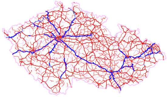
Figure 1.
TMC segments according to RoadType displayed on the map of the Czech Republic.
An important factor for each TMC segment is the FreeFlowSpeed, i.e., the passage speed under ideal weather conditions without any restrictions arising from the density of other traffic or construction restrictions. The FreeFlowSpeed is restricted from exceeding the maximum speed limit arising from traffic regulations for the given road segment. For each of the segments, we can monitor how the actual measured speed deviates from the FreeFlowSpeed.
For each OSM segment, additional information was gained from the OSM, which can affect the traffic flow in the given segment—in particular, the type of road (e.g., motorway, major road network, first class road), the actual length of the segment, the number of public transport lines using this segment, and the number of public transport stops, traffic lights, pedestrian crossings, level crossings, and driving traffic lanes. Not all of these segments had such attributes.
Data assignment from the OSM was carried out automatically, and it must be noted that it was not always entirely accurate. For instance, it is possible for some of the OSM segments comprising 1 TMC segment not to have the identical type of road set. Despite this fact, OSM data helped with the further data processing and some of the inaccuracies have been already corrected. Figure 1 contains the road network on the map of the Czech Republic with colorful highlights of segments depending on their type. The displayed segments only include the road segments in the Czech Republic where traffic information was available (as a result, certain fragments are entirely separated).
Figure 2 contains the frequency of TMC segments according to their RoadType. We distinguished between Motorway (M), Motorway link (ML), Trunk (T), Trunk link (TL), first–third class road (1, 2, 3), their slip roads (1L, 2L, 3L), and finally, Residential (R), Service (S), Track (Tr), and Other (O).
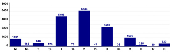
Figure 2.
Frequency of TMC segments according to RoadType.
3.1.2. Traffic Measurement
Real data on traffic measurement in individual road segments in the Czech Republic were available for analysis. The given traffic data were created by the merger of various data which are processed by the Road and Motorway Directorate of the Czech Republic. For the merger of data, the organization uses, in particular, FCD, as well as data from traffic detectors, electronic toll systems, CCTVs, and installed induction loops [47]. The resultant data, which are further distributed as real-time traffic information, contain values of the currently reached degree of traffic saturation, the average speed, and the time necessary for passing the given TMC segment. Values are supplied in minute-resolution in irregular intervals. There is no further publicly available information about gathering and preprocessing of data. This activity is carried out by the Road and Motorway Directorate of the Czech Republic as a state-funded organization established by the Ministry of Transport of the Czech Republic, and it provides no further information with respect to this process, see [47].
Figure 3 illustrates the average number of total traffic measurement per 1 segment and 1 h (thick dark blue line) and according to the individual types of road segments (motorway—black, first class road—violet, residential area segments—green, and the remaining less important types—grey).
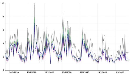
Figure 3.
Average number of measurement sessions per 1 segment and 1 h in the week from 24 February to 1 March 2020.
The number of measurement sessions varies during the course of hours, between the individual days of the week, and between the individual segments. Generally, the maximum frequency is 10 records per hour (for certain motorway segments). On rare occasions, up to 12 measurement sessions are taken at a certain hour and a certain segment. During the night, on weekends, and on holidays, the frequency of measurement sessions is lower. In certain segments, during the night or on weekends, there were no measurement sessions available at all. For more information, see Section 3.2 and Section 4.
3.1.3. Traffic Restrictions: Planned and Unplanned Events
Traffic restrictions concern planned roadworks, unplanned emergencies on the road, and accidents. Traffic restrictions for the given segment were mapped through Tmcld and included the following data: Type of event, event ID and version, driving direction, text description of the event, and event validity end. Thanks to version control, it was possible to ascertain whether the given event changed its status or not (e.g., road closure terminated early).
This information was used primarily for clearing the history, or the elimination of traffic measurements over periods which are not representative due to being misleading (e.g., road closure or traffic accident). In the actual implementation, any restriction on a specific road segment is covered by the navigation application itself, so that the route is not planned through this segment in the event of traffic restriction. Thus, the prediction model is not asked for prediction for this segment.
Due to the fact that this data were available only as of 18 May 2020, an additional test was created to detect periods of abnormal change in the characteristics of the traffic flow in a given segment (see Section 3.2). No data from periods of traffic restrictions were included in the training set.
3.1.4. Meteorological Values
Weather forecast was mapped to each OSM segment (500 m in length at maximum). Forecasts are updated by the provider 4 times per day, at approximately 9.00 a.m., 1.00 p.m., 9.00 p.m., and 1.00 a.m. These forecasts were also collected 4 times per day, and forecasts for each 24 h period were collected. The aim was to ensure there was at least 1 forecast available at every hour per road segment. From time to time, it was not possible, for instance, due to the earlier issuance of a new forecast. The worst-case scenario thus involved a forecast collected 9 h prior to the required time.
The following meteorological data were collected: Time of the forecast collection in hours, outside temperature in °C, wind direction (azimuth) in degrees, wind speed (m/s), air humidity (in %), atmospheric pressure (hPa), cloud amount (in %), fog (in %), low-level clouds (in %), mid-level clouds (in %), high-level clouds (%), dew point in °C, and precipitation amount in the past hour (mm).
3.1.5. Calendar Data
Calendar data constitute a part of the internal memory of the prediction model and store information on the individual days of the year that are important for the quality estimation of traffic density. Primarily, this information states whether a given day is a workday or holiday. For this purpose, the calendar provides information concerning the type of the day per week and whether it is a bank holiday. As for bank holidays, actual strictly defined bank holidays repeated on the same date must be distinguished from bank holidays with moveable dates (this currently involves Good Friday and Easter Monday). The calendar also considered the date of the start and end of the Central European Summer Time (CEST).
Furthermore, the times of sunrise and sunset were pre-calculated for each day of the year. The implementation set forth by the authors of [48] was used for the calculation. The values were saved in Central European Time (CET) and were alternatively transformed to CEST only for the specific year. Due to the fact that the prediction model resolution was in hours (see Section 5), it was only necessary to pre-calculate values for 1 location in the Czech Republic (the selected location was Prague, Old Town Square).
3.2. Data Pre-Processing
Data from the aforementioned main datasets were linked to the segment where they belonged via road segment ID (Tmcld). This link was carried out using the data on the road segment position in World Geodetic System (WGS84) or using special TMC location tables acquired directly from the data provider. Only such road segments which could be mapped to traffic information were used for the prepared analysis. The first issue concerning data understanding was its relatively vast scope, which would not allow the possibility of browsing through the individual segments, let alone the individual FCD measurements.
3.2.1. Hourly Aggregation
The frequency of measurements in individual segments varies significantly. Information from a single FCD measurement about the achieved speed in a given segment will be strongly affected by several individual factors—type of vehicle, nature of load or style of distribution, individual skills of the driver, etc. Consequently, the authors proceeded to aggregate all of the measurements within 1 h of 1 segment into 1 record. This record stores information on the average value of achieved speeds per this specific hour, as well as the range of speeds per given hour (minimum and maximum measured speed). It also stores the number of measurement records acquired for this hour.
Aggregation performed this way decreases significantly the amount of data and, from the perspective of the prediction model, it has a higher information value without any significant loss of detail. Figure 4 illustrates the course of the average hourly speed for the Nusle Bridge in Prague (TmcId: TS04395T04396) in the week from Monday, 24 February, to Sunday, 1 March 2020. The dark blue highlight signifies the average speed per given hour, while the light blue highlight signifies the minimum and maximum speed per given hour. The graph shows the typical daily and weekly development. On weekdays, the measured speed dropped to less than 10 km/h (here, it was entirely due to the traffic density), but it went up at night. On the right, there are data for Saturday and Sunday where the traffic was lower, and the speed was not reduced as much during the day (with the exception of road traffic accident).
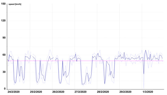
Figure 4.
Example of the course of the average hourly speed for the Nusle Bridge in Prague (TmcId: TS04395T04396).
The range between the lowest and highest measured speed per given hour (light blue lines) represents the variability which cannot be explained by the day of the week or by the hours of the day. Therefore, it makes sense to try to integrate other explanatory variables in the predictions (e.g., weather). Even after aggregation by hours, it must be taken into consideration that, sometimes, there were no measurements available at all per a given hour. This lack of measurements occurred mainly during the night. Sometimes, there were no measurements available per weekends, especially for lower types of roads.
3.2.2. Daily Aggregation
In certain cases, it was suitable to consider even a higher level of aggregation—by days. This allowed us to create a well-arranged display of long time periods—see Figure 5 where the blue highlights signify the average values of the speed in the period from 6 January to 29 June 2020.
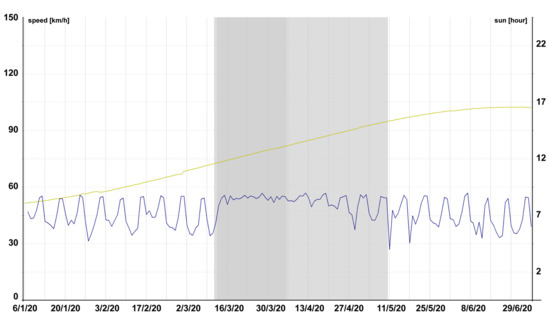
Figure 5.
Example of daily average measured speed and the hours with the sun above the horizon on the Nusle Bridge in Prague (Tmcld: TS04395T04396).
The grey foundation constitutes the period of the state of emergency and ordered quarantine. We can see a clear boundary line during the course of the measured speed and 2 phases of traffic impact—absolute traffic restriction implying the complete loss of weekly profiles (dark grey) and the gradual return back to normal associated with the gradual loosening of the quarantine (light grey). Besides the average daily speed, Figure 5 also shows the development of the number of hours with the sun above the horizon (yellow).
3.2.3. UTC, CET, and CEST
The prediction model and its history always used the currently applicable time. This means that, in the summer, it was CEST, and in the winter, it was CET. This concerns the fact that the traffic density is derived from the currently applicable time. Within data preprocessing, all the time values were transformed from UTC to CET or CEST. Upon transition from CEST to CET in autumn, there would be 2 records per hour from 2.00 a.m. to 3.00 a.m. The first hour (prior to transition to CEST) was thus ignored. The current implementation counts on the fact that the last transition to CEST will be performed in 2021.
3.2.4. Data Cleaning
It was necessary to remove nonrepresentative values from the collected data as they would impair the estimation of the prediction model. This mainly includes measurements in segments undergoing certain traffic restrictions. For this purpose, the dataset of traffic restrictions was primarily used (see Section 3.1). For the time of existence of the traffic restriction, the data were marked as invalid and were not used for the determination of the prediction model.
The problem with the set of traffic restrictions is that it has only been available since 18 May 2020. Prior to this date, there was no credible information available. At the same time, an ad hoc manual check of data implies that at least some of traffic restrictions were not recorded in the traffic restrictions dataset.
As a result, a simple additional test was implemented with respect to suspicious data values, where such values were marked as invalid in the history. The test was based on the detection of sudden decrease in the average daily speed in the given segment (by more than 20% and at least by 15 km/h) lasting at least 3 days, followed by the return to the average daily speed back to the original value. Despite the fact that not all of nonrepresentative data were detected this way, it seems that this detection, along with the official set of traffic restrictions, constitutes an acceptable solution. In the future, we hope that it will be possible to rely on the set of traffic restrictions provided officially.
Figure 6 illustrates an example of detection of invalid values. The dark red highlight illustrates the period where the existence of a traffic restriction was set forth in the available dataset of traffic restrictions (see Section 3.1). Despite the fact that this dataset should contain all restrictions at least since 18 May 2020, this was not the case. The additional test concerning rapid decreases in average daily speed worked, and it identified the likely occurrence of traffic restriction since 7 March 2020 (light red highlight).
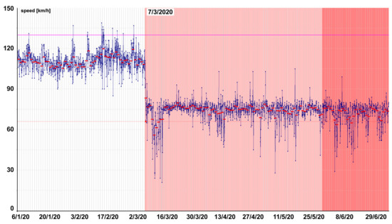
Figure 6.
Example of detection of invalid values. In this case, data for the entire period from 7 March to 29 June were not used for model learning.
All data identified either in traffic restriction or by our additional test were automatically removed from the training data. Moreover, all data from 12 March to 26 April 2020 were removed also from the training data. During this period, the traffic was highly affected by the consequences of the SARS-CoV-2 coronavirus pandemic (COVID-19) due to the measures applied generally in order to prevent the spreading of coronavirus in the Czech Republic.
4. Data Exploration
Due to a significant size of data, the purpose of primary analysis was to determine whether there is some scope for the prediction model to be useful. This means whether there are certain differences at all in the achieved speed in each segment, if so, how large are such differences and whether they vary during the course of the day or night.
Figure 7 illustrates the morning rush hour on roads in the Czech Republic. The deviation between the average speed and the FreeFlowSpeed (the speed without any restrictions) for each segment is displayed in the highlight scale from green to red. The deeper the red, the greater the difference in the speed in the given segment and the given hour. Many segments in red therefore mean that the speed of passing the segment relied on other factors (e.g., weather, holiday). So, it should be possible to improve the prediction model.
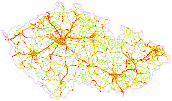
Figure 7.
Example of 1 h (between 6.00 a.m. to 7.00 a.m.) from the period of rush hour on the roads in the Czech Republic.
For illustrative purposes, differences for the whole day are displayed in Appendix A as an online animation on the map of the Czech Republic. Still, the deeper the red, the bigger changes occurred in the average speed. Such segments were the most interesting for the analysis.
Another question was the number of measurements available. Daily aggregations were used for this analysis. Figure 8 shows number of measurements for each individual day in the period from January to June 2020. A lower number of measurements was evident on weekends. At the same time, it was evident that, as of 24 January, a systematic change was made in the means of data collection by the provider as the number of measurements available decreased significantly. The change mainly affected motorways and major road networks (light blue lines at the bottom depicting the individual types of road segments).
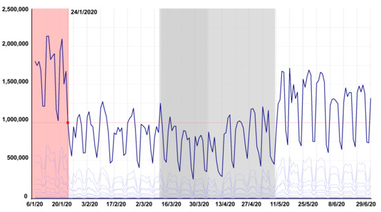
Figure 8.
Number of measurement sessions starting from Monday, 6 January to 29 June 2020.
Next, we looked more closely at difference between the FreeFlowSpeed (as explained in Section 3.1) and average achieved speed. Thus, we obtained the so-called speed difference. The speed difference value of zero means that, on average, on a given day, all vehicles travelled at full speed without any restrictions coming from traffic density or weather. On the other hand, the speed difference value of 10 km/h means that, on average, all vehicles were 10 km/h slower than the theoretically possible speed, i.e., the FreeFlowSpeed for the corresponding road segment. Occasionally, it is possible that the speed difference is below the zero. In some cases, drivers were driving faster than the legal speed limit and thus faster than the FreeFlowSpeed. This occurred especially during night hours on some road segments.
Figure 9 illustrates the daily aggregate deviation from FreeFlowSpeed in absolute values. The average aggregate deviation from FreeFlowSpeed is marked dark blue. Thin light blue lines illustrate the average daily deviation for the individual types of road segments. The highest differences from the FreeFlowSpeed were visible on motorways, reaching 20 km/h or higher. Other road segments speed differences from the FreeFlowSpeed only reached up to 12 km/h. At the same time, we can see a slightly different behavior from the beginning of the year until approximately 13 February 2020.
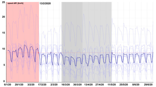
Figure 9.
Daily deviation from FreeFlowSpeed starting from Monday, 6 January, to 29 June 2020.
Figure 10 illustrates the hourly deviation from the FreeFlowSpeed. Minor differences were evident on weekdays and the traffic flow was more fluent on weekends (thus, achieved speeds were near the FreeFlowSpeed). It is also interesting that generally lower speeds were found on motorways at night, which were likely not caused by traffic density but by more careful driving.
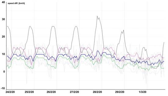
Figure 10.
Hourly deviation from FreeFlowSpeed starting from midnight of 24 February to 1 March 2020.
Figure 11 illustrates the average hourly deviation expressed relatively to FreeFlowSpeed. Using the relative speed differences allowed for a better comparison among heterogeneous types of road segments with significantly varied FreeFlowSpeeds (e.g., motorways and residential roads). We can see here that, during the rush hour, the slowdown was relatively most common on the first class roads (violet highlight line) as opposed to motorways (thick black line), where a slowdown on night was still recognizable.
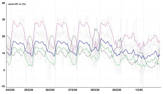
Figure 11.
Relative hourly deviation from FreeFlowSpeed starting from 24 February to 1 March 2020.
5. Design of Prediction Model
Individual measurements of achieved speed are affected by a number of factors, and the current traffic density is only one of them. The speed is certainly also affected by the type and condition of the vehicle, nature of the load, individual skills of the driver, whether the driver is in a rush, whether it was necessary to stop somewhere within the segment (e.g., for delivery of goods), and so on. We can assume that the drive speed is also affected by the time of day or night and the current weather, especially some extreme weather conditions (heavy rain, dense fog, black ice…). Traffic can also be affected by collective decisions of people who might prefer commuting in their air-conditioned cars on very hot days over commuting by public transport. Traffic density is highly affected by the type of day (day of week and, most importantly, whether it is a workday or holiday). Traffic density can be affected by school holidays (especially summer holidays), but these have not been included among the data so far. Certain factors can be contradictory—it is possible to drive faster at night due to lower traffic density. However, reduced visibility forces the driver to drive slower.
When designing the model, we were generally restricted by the relatively short history which was currently available, and also by the fluctuation in the measurement frequency. This led to increased emphasis to making the model robust so that its results were not significantly skewed by a single outlier measurement. At the same time, real-world usage conditions must be taken into account. For instance, records of measurements will not be available real-time for our purposes, but in batches and with a delay of at least several weeks or months. It must not be excluded that history updates will only be performed once per year. This means that an autoregressive model cannot be used. On the other hand, we can count on the fact that the prediction model will be used as a supplementary one. Therefore, it is possible to issue prediction only when a high accuracy of the estimation can be expected.
The preliminary data analysis revealed that the TMC segments were very individual as each of them had its individual profile of achieved speeds on a given day of the week. We cannot rule out that a longer history in the future will reveal certain global characteristics, but so far, the best option seems to be to create a separate prediction model for each TMC segment. This also corresponds with the expected use of the prediction model, where the navigation system will request the predictions on segments in a given route one by one.
5.1. Choice of Prediction Technique
As there were over 20,000 TMC segments, a suitable prediction technique must be considered which will be capable of handling and maintaining such a large number of models. We cannot rule out even a more frequent update of history data in the future and thus more frequent retraining of models necessary for some types of prediction methods.
The following prediction techniques arising primarily from the initial research were considered:
- Case-based reasoning (CBR), a nonparametric approach,
- Linear regression (LinR), a parametric approach, and
- Artificial neural networks (ANN), a nonparametric approach.
The advantages of CBR include explicability, predictability, robustness, automatic model update, and fast adaptation to changes in behavior. Nevertheless, it is evident that it cannot detect all fluctuations in data and is less accurate. The main advantage of ANN is that, if fitted properly, it can describe data behavior very well. However, there is a significant disadvantage in explainability of results because the neural network is a “black box.” Moreover, it has high requirements for training each individual model and is also relatively prone to “overfitting” to specific data. The main issue for LinR is the relatively short history for a proper setting of regressive parameters.
After consideration, the CBR technique was selected as the primary one mainly due to its robustness and, last but not least, to the easy of explanation of its results. If a sufficiently long history is available for a given segment, the linear regression can be used as a more precise prediction involving other influences, including the weather. Still, the expected speed is computed first by means of CBR and serves as an “anchor” for the detection of cases where the linear regression provides an unlikely value or fails entirely to solve matrix equations.
5.2. Conceptual Scheme of Prediction System
Figure 12 illustrates a conceptual scheme of the prediction system which implements the designed prediction model and ensures the communication with other systems (see Section 7). The prediction system uses ensemble prediction model consisting of three submodels.
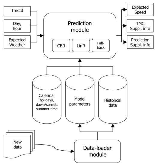
Figure 12.
Conceptual scheme of prediction system.
According to the Tmcld and the precise determination of hour for which the prediction is to be issued (and possibly also according to the expected weather at the given time), the system will issue a prediction of the expected speed.
In order to extend the possibilities of processing the results, other supplementary information is provided at the output: The TMC supplementary information (value of FreeFlowSpeed per given segment and the length of such a segment in meters) and the Prediction supplementary information (code of the used submodel, the minimum and maximum speed recorded for the given segment at the given hour, the number of individual measurements in the history, and the number of hours for which there is at least one measurement available).
Based on the analysis performed before, it was determined that it was not necessary to create a model for the period from 10 p.m. to 5.00 a.m. On the one hand, only a limited number of measurements was available. For another, the achieved speeds in this period were mostly affected by other factors than traffic density. An example is the identified slowdown on nights on motorways. Despite being evident from the data, it is insignificant for the purposes of navigation and when planning the route (roads are empty at night). A backup prediction is available for these hours, which was implied from the theoretical value attainable in the given segment (FreeFlowSpeed)—see Section 5.5.
5.3. CBR Submodel
This technique is based on the selection of a subset of representative cases from the available history. As for the prediction of expected speed, the type of day and hour were identified as the two most important factors. From the available history of hourly aggregated values for the given TMC segment, such records are selected which concern the same hour for which the prediction is to be issued, which are also the hours of the same type of day.
When selecting the same type of day, the model distinguishes between workdays and days off. As for workdays, it distinguishes each day between Monday to Friday, and as for the days off, it considers Saturday and Sunday. For less frequent types of days (Friday or Monday bank holidays…), selection is made of a similar type of day, so that it is possible to find a sufficient number of examples in the history.
Due to an insufficiently long history and the attempt to increase the number of representative cases, the original implementation considered workdays in the middle of the week (Tuesday, Wednesday, Thursday) as identical ones. However, this revealed a negative impact on the prediction accuracy as the development of traffic density is different even between these individual days.
Prediction of speed upon passing a TMC segment was subsequently calculated as the average value of hourly speeds out of all representative cases in the currently selected subset of historical data:
where
- PCBR(hour) is prediction of average speed for a given segment at the “hour”;
- Nh is number of records in history for the given TMC segment;
- Si is average hourly speed from an i-th record in the history;
- Φ(i, hour) is Boolean function of similarity providing values of {0,1} depending on whether the i-th record in the history is for the same hour and the day of the week as the “hour” the prediction is currently made for:
where
- Hour(Si) is hour for which the speed Si was measured,
- Dayofweek(Si) is type of day of the week for which the speed Si was measured,
- Dayofweek(hour) is function providing the type of the day in the week for the hour for which the prediction is being calculated.
The identification code for this submodel is CBRBasic. Besides the actual prediction, both the lowest and highest achieved speed in the current subset of all representative cases is provided in Prediction supplementary information, so that it is possible to infer how the actual speed can vary.
5.4. Submodel Linear Regression (LinR)
This model attempts to include influences of other factors in the prediction. Provided that there are enough representative cases available in the subset for a given hour in a given segment (see the similarity function Φ(i, hour) above), we use multiple linear regression with vector xi of explanatory variables and dependent variable yi.
where
- nh* is number of records from history for which it applies Φ(i, hour) = 1 (see above);
- where
- Trendi is order number of the day (calculated as of 1 January 2020),
- Seasoni = 2 × Π × DayOfYearIndex(Si)/365 is normalized order number of the day in the year, and
- Suni is fuzzy function providing the coefficient of sun-above-the-horizon period for the hour of i-th record as follows:
- ⟨0;1⟩ …for the period of 60 min before and upon sunrise as at HH:30,
- ⟨0;1⟩ …for the period of 60 min before and upon sunset as at HH:30,
- otherwise, 0 if the sun is below the horizon and 1 if sun is above the horizon for the entire hour;
- is relative average hourly speed. Dividing by the value of the FreeFlowSpeed does not affect the prediction quality. Instead, it only ensures that the calculated regression coefficients are mutually comparable between the individual TMC segments;
- εi is random file (prediction error).
The vector on the left side is currently created by the following components: Mean value, trend, season, and information on whether the sun is above the horizon (see Section 3.1). The last component solely applies to hours where there is a change during the course of the year between the summer and winter solstice, e.g., it will be completely dark outside at 7 p.m. in the winter, yet the sun will be well above the horizon in the summer. As opposed to that, at noon and at midnight hours, this vector component contains only the same values and is thus eliminated automatically.
After that, we tried to find a vector of regression coefficients to minimize the sum of squares of random noise εi, using the least-squares estimation method:
Finally, an expected relative speed was computed as a dot-product of vector of regression coefficients and vector of explanatory variables for the hour the prediction is made for:
Linear regression coefficients were computed relatively to the FreeFlowSpeed (for the vector to be comparable among road segments—see yi above). Therefore, the dot-product must be multiplied by the FreeFlowSpeed to obtain an expected speed in km/h:
The identification code for this submodel is LinRBasic. Submodel CBRBasic still remains as a backup model when there are not enough representative cases in the subset and linear regression fails. At the same time, the value provided by the CBRBasic submodel serves as an “anchor” to identify situations when the linear regression results are not to be trusted. For instance, prediction by linear regression must not exceed the permitted deviation from the value acquired from the CBRBasic submodel or must not exceed the range between the minimum and maximum measured speed at this hour (as provided in the Prediction supplementary information).
5.5. Fallback Submodel
Last but not least, we must take into account the situations where the usable history is too short to provide a sufficient forecast even for the CBRBasic submodel. For certain segments, days of the week, and specific hours, no measured value is available at all (especially at night or at weekends). The only available piece of information for such situations is the FreeFlowSpeed value for the given segment. The prediction is then be provided according to a simple equation:
where kF is the correction coefficient. The simplest variant is that kF = 1.0. The fallback submodel is used if there are less than three records available in the history, or if the records in the history are based on less than 20 records of individual measurements (the number was determined on an experimental basis). The identification code for this submodel is NoDataFallback.
For the period from 10.00 p.m. to 5.00 a.m., it was not traffic density, but individual factors which mainly influenced the achieved speed. At nights, the speed was reduced, especially on motorways. For the majority of cases, this does not mean that the traffic was too dense to prevent any higher speed, but that the drivers themselves slowed down due to reduced visibility or fatigue. At the same time, fewer measurements were generally available in history. Based on the analyses carried out so far, the coefficient value for hours of night was set to kF = 0.9. Bearing in mind a planned purpose of the prediction model to support a navigation system, for the hours of night (with order numbers 0, 1, 2, 3, 4, 22, and 23), this fallback submodel was used as the primary submodel. The identification code for this submodel is NightFallback.
5.6. Linear Regression Using Meteorological Data
Based on earlier analysis of data, it was observed that the difference between the lowest and highest measured speed in a given hour represents could not be explained by the day of the week or by the hour of the day only. Therefore, it makes sense to try to integrate other explanatory variables into the predictions, such as the weather.
We tried various ways to extend the linear regression using the weather. We tried instantaneous values, as well as their moving average values for the past 3 to 12 h. Unfortunately, the results were very weak. It seems that the average temperature value did not provide any added information. We tried to limit any extreme temperatures and to concentrate only on temperatures around zero or moving averages. None of this brought any prediction improvement. On the contrary, there was significant deterioration in most of the situations.
This is similar even with other meteorological data available. We tried aggregate values, e.g., visibility as a combination of the sun-above-the-horizon coefficient, cloud amount and fog, or black ice as precipitation for temperature around 0 °C. However, nothing improved the prediction.
The only exception was the total amount precipitation in the past 6 h (or the moving average for the same period), where the prediction improved slightly yet visibly. Nevertheless, the improvement was not as significant for the model to be extended by this input. Every new input constitutes a risk that the robustness of the model is decreased and there is also the issue concerning the weather forecast error. Due to this, the weather was not included in the model at this point.
We can explain the meteorological data issue with the following causes:
- First, only a very short history (6 months and approximately 20 cases per each day of the week and the given hour) was available, so excessive expansion of vectors of explanatory quantities either led to the overfitting of linear regression, or the number of historical cases even dropped below the number of explanatory quantities (in such a case, there is not a single solution, thus the linear regression cannot be calculated).
- Second, winter 2019/20 was extremely mild in the Czech Republic, thus low temperatures were not sufficiently shown among the data. At the same time, the precipitation amount was relatively low or, more precisely, the precipitation amount in spring reached nearly zero. Fog occurrence was also only minimal.
The situation could be improved once there are data available over a longer period of time and provided that the weather is more variable. At the same time, we need consider the fact that there is only a weather prediction available rather than an actual measurement. Albeit the short-term (in units of hours) weather forecast is very accurate, it may not detect all actual phenomena or their intensity (e.g., precipitation).
6. Validation of Designed Model
The current version of the prediction model (i.e., not including the meteorological values) was tested using all the data currently available. The period from 7 January to 14 June 2020 was used as a training set (data in the model history were only used for learning). Prediction was tested using the week from 15 June (Monday) to 21 June (Sunday) as the last week in June was affected by the upcoming start of summer holidays and by people going away. Data collected after 22 June have not been used so far.
We need to emphasize that a proper testing of the model was undertaken with the testing period and did not include the history used for the model training. Furthermore, any nonrepresentative values were automatically eliminated in advance from the data used for model training. This mainly comprised various traffic restrictions (see Section 3.2) and the period of state of emergency, or the period of the strictest ordered quarantine in association with COVID-19, which caused a decrease in traffic density from 12 March to 26 April 2020.
The testing methodology was stated as follows:
- No testing was performed with respect to prediction for night from 10.00 p.m. to 5.00 a.m.
- Prediction could only be calculated for hours where there was at least one traffic measurement available for the given TMC segment.
- The main metric was the absolute difference between the predicted speed and the measured average speed (prediction error) for a given hour.
We used the mean absolute error (MAE) metric to evaluate the absolute error between the prediction and real values for a given road segment. MAE was defined as:
where Si means the real average speed for hour i, Pi denotes the speed prediction for the same hour, and np is the number of samples in the test set.
Summary results of testing of all 20,504 TMC segments is as follows:
- MAE of all the individual predictions (across all TMC segments) was 4.67 km/h with a standard deviation of 1.642 km/h.
- Average of MAE of the individual TMC segments (with at least one prediction) was 4.91 km/h, with a standard deviation of 1.996 km/h.
- In 90% of cases, the average error per all TMC segments was below 10.80 km/h.
- In 95% of cases, the average error per all TMC segments was below 14.01 km/h.
- In 87.93% of all predictions, the average absolute prediction error was below 10 km/h.
- The average maximum prediction error per all TMC segments was below 24.02 km/h.
Appendix B contains a text file with a complete overview of all segments and their testing results.Table 2 illustrates a selection of TMC segments from Appendix B, which are introduced in more detail in Figure 13, Figure 14, Figure 15, Figure 16, Figure 17, Figure 18, Figure 19 and Figure 20.
Table 2.
Selection of TMC segments and stated data concerning prediction error.
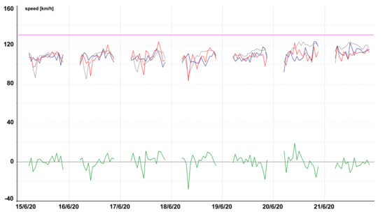
Figure 13.
Model testing on motorway, D1 near Průhonice (Tmcld: TS04633T25530).

Figure 14.
Model testing on city primary road, Prague—Nusle Bridge (Tmcld: TS04395T04396).
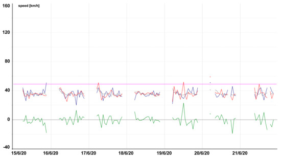
Figure 15.
Model testing on city secondary road, Prague—Legions Bridge (Tmcld: TS05567T05566).
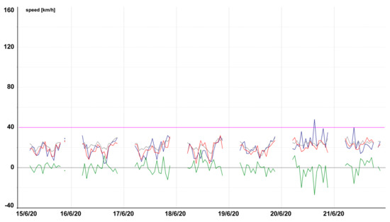
Figure 16.
Model testing on secondary road, local street in Přerov (Tmcld: TS37339T13546).
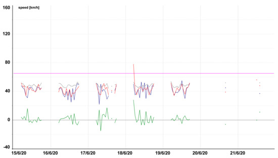
Figure 17.
Model testing, segment where there is basically no data available at the weekend, secondary local road in Nechanice (Tmcld: TS12627T12626).
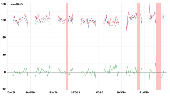
Figure 18.
Model testing, prediction for a segment with commonly occurring traffic restrictions, motorway D11 near Chrast (Tmcld: TS23996T25618).
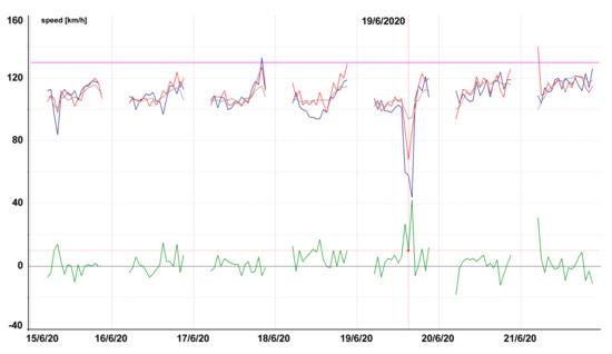
Figure 19.
Model testing, linear regression attempts to detect the Friday rush hour, Motorway D1 passing by Brno (Tmcld: TS01318T01319).
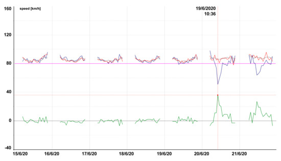
Figure 20.
Model testing, trunk road Nr. 43 in Brno (Tmcld: TS05024T04030).
In Table 2, column Count contains the number of hours for which testing could have been performed. The testing week spanned 168 h, but prediction was not tested at night from 10.00 p.m. to 5.00 a.m. (other factors than traffic density influence achieved speed). Thus, the maximum number of predictions was 119. A lower number indicated that, for some hours, there were no speed measurements available.
Column MAE contains the mean absolute error (difference of the predicted speed from the average measured speed one). Columns Err90pct and Err95pct contain the maximum value of absolute difference in 90% and 95% of cases, respectively. Column ErrMax contains the maximum value of absolute difference. Column Low contains the number of cases where the prediction difference was below 10 km/h. In column Low %, this number of cases is expressed relatively to the value contained in column Count.
Figure 13, Figure 14, Figure 15, Figure 16, Figure 17, Figure 18, Figure 19 and Figure 20 contain graphic expressions of the average measured speed (blue), predicted speed (red), FreeFlowSpeed (violet), and prediction error (green) for the selected road segments from Table 2 for each hour of the testing week from Monday, 15 June, to Sunday, 21 June. For illustrative purposes, prediction according to the CBR model is in grey. We can see that the use of linear regression led to a more accurate prediction in the majority of cases.
In Figure 20, the model did not manage to detect the weekend decrease, but it accurately predicted the continuous exceeding of the permitted speed on workdays.
7. Conceptual Design of Using the Proposed Solution in the Navigation
In this article, the designed prediction system (see Section 5.2) can be implemented into navigation and fleet and workflow management systems as one of the modules often used for route calculation. The stated systems have their own solutions to ensure navigation. The main benefit of the prediction system is, in particular, route optimization with respect to the predicted traffic situation (and possibly also weather forecast) where the route is planned via waypoints (see problem context in Section 1). Besides the primary use, this prediction system can be beneficial even to navigation between two points, similarly to speed profiles, making the estimated arrival time more accurate. Furthermore, the basic principle of involving such a prediction system or module into the aforementioned systems (their navigation part) is beneficial as the calculated routes can be optimized according to the traffic prediction and weather forecast.
Based on the selected goal and waypoints, navigation or the relevant system module creates a virtual subgraph from map bases, above which alternative routes will be calculated further for the current departure time. The individual edges of the virtual subgraph have signs of TMC segments for which real-time traffic information is available. Real-time traffic information is downloaded for all TMC segments (generally primary roads) in this subgraph from the place of departure. Subsequently, route calculation is performed according to the selected heuristic algorithm. In the event of a TMC segment, any penalization based on real-time traffic information is included.
If the route is longer than, let us say, 30 min (the value will need to be set on an experimental basis), all TMC segments attained at a later point will be penalized based on the prediction system data and not based on real-time traffic information. If several waypoints are used, the route can be penalized right from the first waypoint based on the prediction system data. As indicated by Figure 21, the initial data (Tmcld, passage date, estimated time of passage through the segment rounded to hours) will be passed onto the prediction system. At the same time, such TMC segments with long-term traffic restrictions (e.g., closed road) will be eliminated from the initial data by the navigation based on real-time traffic information. The prediction system will provide values of the predicted speed for the individual TMC segments as well as supplementary information (see Section 5.2). Upon route calculation completion, the user will be offered a suitable route(s), which will be displayed on the map. During the course of travel, the navigation will recalculate the given route continuously through the given time and, if necessary, it will offer an alternative route.
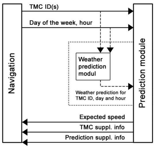
Figure 21.
Conceptual design of integrating the prediction module into navigation.
As illustrated by Figure 21, the initial data also contains a weather forecast for the expected passage time. Due to the fact that an added value of using the weather forecast in the designed prediction model has not been proven, Figure 21 illustrates the use of weather in the conceptual design as optional—see issues with including such data as set forth in Section 5.6 and Section 8. The inclusion of weather forecast can be performed in the form of a separate module or as a part of the prediction system. The advantage of the separate weather module is its usage for depicting the current weather and the forecast on the navigation map or, alternatively, its further separate use outside the prediction system.
8. Discussion and Future Directions
Generally speaking, there is a number of specific conditions (e.g., social and technological aspects of the application environment, local availability, and quality of data inputs) which restrict the defined goals of the designed model focused on traffic prediction and related indicators. To a certain extent, contextual conditions related to research or application affect the success rate of models designed within a different task and a similar problem context where they may not reach as accurate results. This is also associated with the performed validation of the designed solutions. For instance, validation of the designed solution of testing data from a very limited temporal or spatial segment of the road network or in specific geographic conditions of the given region (e.g., region with low precipitation) only provides a framework perspective of suitability of using the specific prediction model in practice.
This is how the artefact design issue is also approached by design science [42], which tries to offer paralogy of perspectives and approaches on handling a specific problem context. Experienced professionals then make the final selection of the most purposeful solution, which is not necessarily the most suitable one, for instance, from the perspective of attained prediction error rate or used technology (but the selected solution may be easier to implement in a sociotechnical context).
Based on the validation results of the prediction model, we can state that traffic speed is predicted satisfactorily by the model in a long-term perspective. The achieved results may be compared with those found by the authors of [49], who tested the actual model (built-on machine learning) in a mid-sized city. This model achieved approximately 75% accuracy for a reasonable 10 km/h difference and up to 80% accuracy for a 20 km/h difference. Similarly to our case, historical data were primarily collected as FCD.
The multiscale spatiotemporal feature learning network (MSTFLN), introduced by the authors of [19] and tested on three selected motorways and data collected from loop detectors, might serve as another model for framework comparison. The achieved average MAE per given hour is 5.72 km/h, which we consider as comparable with the prediction model introduced in this article. Similar results can also be achieved based on the MAE described by the authors of [50]. The CNN-LSTM model of the authors consists of convolutional neural networks and long short-term memory models, and achieved similar results with respect to real-world dataset of Hong Kong as MSTFLN (the MAE for hourly prediction was 5.4 km/h). Nevertheless, while the prediction of MSTFLN is in hours, the prediction of the CNN-LSTM model is restricted to dozens of minutes. Very good results for the short-term prediction were found by the authors of [51], who presented the attention-based LSTM (ATT-LSTM) model for short-term traffic speed forecasting. The average MAE of their ATT-LSTM model was 3.26 km/h for 15 min prediction.
As for the stated comparison, the restriction with respect to the difference of the used datasets must be taken into consideration. Despite this restriction, based on validation, we consider the prediction model provided in this article as purposeful according to design science (i.e., applicable in practice and achieving reasonable results). Nevertheless, it should be emphasized that the solution presented in this article is for long-term prediction and serves mainly as a supplementary solution to enrich traffic information for better route calculation in car navigation systems.
There were also some restrictions in the research introduced in this article, which were caused by the problem context in which the designed solution should be included within the applied research project. From the perspective of design research, it is beneficial to introduce the actual procedure for the solution by which other researchers may be inspired when using other algorithms, methods, or approaches to the solution [52]. Even in association with other views of using parametric or nonparametric approaches and their suitability for certain conditions introduced in Section 2, the authors would also like to emphasize the unique particularities associated with the performed research:
- Available historical traffic data was based on data merger from various sensors (e.g., FCD data can be less accurate than data from the inductive-loop sensor in the same segment).
- Available historical traffic data concerning traffic measurement covered 66% of all road segments in the Czech Republic, i.e., 37,002 km (excluding roads with low rates of vehicle passage).
- The designed model focuses on a long-term perspective while predicting the speed within days and weeks and is thus a macro-spatial and temporal prediction model.
- The designed model is suitable for (car) navigation application and is of a supplementary nature for route calculation, see Section 7.
The stated contextual particularities differ significantly from the contextual particularities of models introduced in articles set forth in Section 2. Based on the aforementioned, we can say that, from a long-term perspective and considering the vastness of the territory, ensemble models based on data-driven statistical and machine learning approaches can reach very good results similarly to using deep learning approaches. The achieved good results of the prediction model can be explained by the following facts:
- Average speed was predicted for a given hour of the day.
- Night hours (from 10.00 p.m. to 5.00 a.m., see Section 5.2) were excluded,
- The model considered only segments with no reported traffic restrictions.
- Data were available for the model just right before the start of the testing period.
The inclusion of data concerning weather (forecast) can be considered as a logical step as the weather affects many aspects of road conditions and safety and is reflected in traffic speed and the values associated therewith (e.g., flow, density). The aforementioned is supported by the research conducted by the authors of [49] and [53], in which the designed models indicated the benefits of implementing weather data into traffic state prediction. The authors of [39] used a specific ensemble model based on deep belief networks for the improvement of traffic flow prediction, which indicated that this model, which used weather data from a short-term perspective, provided better results than models based solely on historical traffic data. However, this study did not provide a long-term prediction in days and within various categories of roads as in our case, and instead only focused on 47 selected freeways in California. Inductive-loop sensors serve as data sources rather than FCD primarily and secondarily merged data from other sensors. This is also associated with the number of measurement sessions for the individual segments, which may not be regular. All of this can affect the success rate of using weather data for the improvement of traffic state prediction. Similarly, the authors of [54] found that using deep learning-based approaches and ensemble learning while involving weather data enabled very good predictions, especially in hours.
However, weather data has not been implemented successfully in the aforementioned prediction model. Similarly to the results found by the authors of [55], no positive impact on the improvement of parametric models prediction was detected with respect to the majority of weather events. Precipitation was as exception. However, due to the fact that, based on our data exploration, there was a significant dispersion between the minimum and maximum speed, there is still hope that there are actually other explanatory variables, such as weather data, and that the model can still be improved. In the future, besides the weather, it would be interesting to see how likely it is for traffic speed to be slowed down by fixed elements, such as public transport stops, pedestrian crossings, and traffic lights extracted from OSM.
From the perspective of further development of our designed model and its planned implementation into the specific contextual conditions in the areas of car navigation and fleet and workflow management systems, acquiring longer data history for at least a whole year is a further option. Furthermore, we could try to implement the weather-related data to the longer history.
Based on the analysis of data concerning the weather and traffic over a longer period of time, it is possible to find correction coefficients which are generally applicable (e.g., day of the year or weather event) and which could be used in the CBR submodel. Coefficient kF can be increased or decreased this way (it will be possible to add up penalization and bonus awards):
- Rain/snow: −0.1
- Fog: −0.1
- Black ice (temperature around 0 °C): −0.2
- As opposed to that, the period of school holidays can result in a bonus award for this period: +0.1.
Further development concerning the used prediction system will also be associated with the issue of obsolescent data history. In fact, it is possible that, in practice, the prediction system will predict speed only for a given hour based on data collected up to a year before the prediction. It is certainly appropriate to consider the possibility of updating data more frequently, ideally up to the form of its online upload. It would be more demanding on the system operation, but offers several advantages:
- Detection of current changes (e.g., roadworks, opening of new segments).
- Detection of traffic accidents.
- Possibility to select better historical examples based on the initial development of the daily scheme (e.g., depending on the development of attained speed, the most similar day will be selected from the history).
On the other hand, the first two points are ensured by the navigation systems alone as they already use real-time traffic information, so it is not necessary to duplicate this function.
Author Contributions
Conceptualization, M.S. and Z.S.; methodology, M.S. and Z.S.; software, M.S.; validation, M.S.; formal analysis, M.S.; investigation, M.S. and Z.S.; resources, Z.S.; data curation, Z.S.; writing—original draft preparation, M.S. and Z.S.; writing—review and editing, M.S. and Z.S.; visualization, M.S.; project administration, Z.S.; funding acquisition, Z.S. All authors have read and agreed to the published version of the manuscript.
Funding
The authors received public financial support for this research from grant TH04010350 administered through the Technology Agency of the Czech Republic. The paper was processed with support from an institutional fund IP400040 for long-term conceptual development of science and research and internal grant F4/1/2019 at the Faculty of Informatics and Statistics, Prague University of Economics and Business.
Institutional Review Board Statement
Not applicable.
Informed Consent Statement
Not applicable.
Data Availability Statement
The data used in this study are available on reasonable request from the corresponding author only for research purpose. The data are not publicly available due to contracts between the providers of some datasets and our research team. The data supporting the validation presented in this study are openly available in Zenodo at https://doi.org/10.5281/zenodo.4372333, reference number [56].
Conflicts of Interest
The authors declare no conflict of interest.
Appendix A
Examples of the deviation between the average speed and the FreeFlowSpeed for selected hours:


Figure A1.
The animation is at [56]: https://doi.org/10.5281/zenodo.4372333.
Figure A1.
The animation is at [56]: https://doi.org/10.5281/zenodo.4372333.


Appendix B
The text file provides a complete overview of all road segments on which basis summary test results were calculated in Section 6. The text file is at [56]: https://doi.org/10.5281/zenodo.4372333.
References
- Waisley, M.; Zeng, H.; Murtha, S.; Unholz, S. A Next Generation Advanced Traveler Information Precursor System (ATIS 2.0 Precursor System) Use Cases Report; U.S. Department of Transportation: Washington, DC, USA, 2017. [Google Scholar]
- Alobaidi, M.K.; Badri, R.M.; Salman, M.M. Evaluating the Negative Impact of Traffic Congestion on Air Pollution at Signalized Intersection. IOP Conf. Ser. Mater. Sci. Eng. 2020, 737, 012146. [Google Scholar] [CrossRef]
- Baghestani, A.; Tayarani, M.; Allahviranloo, M.; Gao, H.O. Evaluating the Traffic and Emissions Impacts of Congestion Pricing in New York City. Sustainability 2020, 12, 3655. [Google Scholar] [CrossRef]
- Muneera, C.P.; Karuppanagounder, K. Economic impact of traffic congestion- estimation and challenges. Eur. Transp. 2018, 68, 5. [Google Scholar]
- Sweet, M. Traffic Congestion’s Economic Impacts: Evidence from US Metropolitan Regions. Urban Stud. 2013, 51, 2088–2110. [Google Scholar] [CrossRef]
- Li, L.; Qu, X.; Zhang, J.; Wang, Y.; Ran, B. Traffic speed prediction for intelligent transportation system based on a deep feature fusion model. J. Intell. Transp. Syst. 2019, 23, 605–616. [Google Scholar] [CrossRef]
- Wang, J.; Chen, R.; He, Z. Traffic speed prediction for urban transportation network: A path based deep learning approach. Transp. Res. Part C Emerg. Technol. 2019, 100, 372–385. [Google Scholar] [CrossRef]
- Liu, D.; Tang, L.; Shen, G.; Han, X. Traffic Speed Prediction: An Attention-Based Method. Sensors 2019, 19, 3836. [Google Scholar] [CrossRef]
- Niu, K.; Zhang, H.; Zhou, T.; Cheng, C.; Wang, C. A Novel Spatio-Temporal Model for City-Scale Traffic Speed Prediction. IEEE Access 2019, 7, 30050–30057. [Google Scholar] [CrossRef]
- Budimir, D.; Jelušić, N.; Perić, M. Floating Car Data Technology. Pomorstvo 2019, 33, 22–32. [Google Scholar] [CrossRef]
- Sunderrajan, A.; Viswanathan, V.; Cai, W.; Knoll, A. Traffic State Estimation Using Floating Car Data. Procedia Computer Science 2016, 80, 2008–2018. [Google Scholar] [CrossRef]
- Wu, P.; Liu, K.; Hao, S.; Zhang, Q.; Tan, Y. Rapid traffic congestion monitoring based on floating car data. Comput. Res. Dev. 2014, 51, 189–198. [Google Scholar]
- Topolšek, D.; Čižiūnienė, K.; Cvahte Ojsteršek, T. Defining transport logistics: A literature review and practitioner opinion based approach. Transport 2018, 33, 1196–1203. [Google Scholar] [CrossRef]
- Lin, L.; Li, J.; Chen, F.; Ye, J.; Huai, J. Road Traffic Speed Prediction: A Probabilistic Model Fusing Multi-Source Data. IEEE Trans. Knowl. Data Eng. 2018, 30, 1310–1323. [Google Scholar] [CrossRef]
- Abdulhai, B.; Porwal, H.; Recker, W. Short-Term Traffic Flow Prediction Using Neuro-Genetic Algorithms. J. Intell. Transp. Syst. 2002, 7, 3–41. [Google Scholar] [CrossRef]
- Georgescu, L.; Zeitler, D.; Standridge, C.R. Intelligent transportation system real time traffic speed prediction with minimal data. J. Ind. Eng. Manag. 2012, 5. [Google Scholar] [CrossRef]
- Zang, D.; Ling, J.; Wei, Z.; Tang, K.; Cheng, J. Long-Term Traffic Speed Prediction Based on Multiscale Spatio-Temporal Feature Learning Network. IEEE Trans. Intell. Transp. Syst. 2019, 20, 3700–3709. [Google Scholar] [CrossRef]
- Oh, S.; Byon, Y.-J.; Jang, K.; Yeo, H. Short-term travel-time prediction on highway: A review on model-based approach. KSCE J. Civ. Eng. 2017, 22, 298–310. [Google Scholar] [CrossRef]
- Zang, D.; Fang, Y.; Wang, D.; Wei, Z.; Tang, K.; Li, X. Long Term Traffic Flow Prediction Using Residual Net and Deconvolutional Neural Network. In Pattern Recognition and Computer Vision; Springer: Berlin/Heidelberg, Germany, 2018; pp. 62–74. [Google Scholar] [CrossRef]
- Zhang, K.; Zheng, L.; Liu, Z.; Jia, N. A deep learning based multitask model for network-wide traffic speed prediction. Neurocomputing 2020, 396, 438–450. [Google Scholar] [CrossRef]
- Smith, B.L.; Williams, B.M.; Keith, K.O. Comparison of parametric and nonparametric models for traffic flow forecasting. Transp. Res. Part C Emerg. Technol. 2002, 10, 303–321. [Google Scholar] [CrossRef]
- Lefevre, S.; Sun, C.; Bajcsy, R.; Laugier, C. Comparison of parametric and non-parametric approaches for vehicle speed prediction. In Proceedings of the 2014 American Control Conference, Portland, OR, USA, 4–6 June 2014. [Google Scholar] [CrossRef]
- Hamed, M.M.; Al-Masaeid, H.R.; Said, Z.M.B. Short-term prediction of traffic volume in urban arterials. J. Transp. Eng. 1995, 121, 249–254. [Google Scholar] [CrossRef]
- Ahmed, M.S.; Cook, A.R. Analysis of freeway traffic time-series data by using box-jenkins techniques. Transp. Res. Rec. 1979, 722, 1–9. [Google Scholar]
- Mai, T.; Ghosh, B.; Wilson, S. Short-term traffic-flow forecasting with auto-regressive moving average models. Proc. Inst. Civ. Eng. Transp. 2014, 167, 232–239. [Google Scholar] [CrossRef]
- Duan, P.; Mao, G.; Zhang, C.; Wang, S. STARIMA-based traffic prediction with time-varying lags. In Proceedings of the IEEE 19th International Conference on Intelligent Transportation Systems (ITSC), Janeiro, Brazil, 1–4 November 2016. [Google Scholar] [CrossRef]
- Chandra, S.R.; Al-Deek, H. Predictions of Freeway Traffic Speeds and Volumes Using Vector Autoregressive Models. J. Intell. Transp. Syst. 2009, 13, 53–72. [Google Scholar] [CrossRef]
- Mir, Z.H.; Filali, F. An adaptive Kalman filter based traffic prediction algorithm for urban road network. In Proceedings of the 12th International Conference on Innovations in Information Technology (IIT), Al Ain, UAE, 28–29 November 2016; pp. 1–6. [Google Scholar]
- Dong, X.; Yu, Z.; Cao, W.; Shi, Y.; Ma, Q. A survey on ensemble learning. Front. Comput. Sci. 2020, 14, 241–258. [Google Scholar] [CrossRef]
- Clark, S. Traffic prediction using multivariate nonparametric regression. J. Transp. Eng. 2003, 129, 161–168. [Google Scholar] [CrossRef]
- Zhang, L.; Liu, Q.; Yang, W.; Wei, N.; Dong, D. An Improved K-nearest Neighbor Model for Short-term Traffic Flow Prediction. Procedia Soc. Behav. Sci. 2013, 96, 653–662. [Google Scholar] [CrossRef]
- Cai, P.; Wang, Y.; Lu, G.; Chen, P.; Ding, C.; Sun, J. A spatiotemporal correlative k-nearest neighbor model for short-term traffic multistep forecasting. Transp. Res. Part C Emerg. Technol. 2016, 62, 21–34. [Google Scholar] [CrossRef]
- Zhang, Y.; Xie, Y. Forecasting of Short-Term Freeway Volume with v-Support Vector Machines. Transp. Res. Rec. J. Transp. Res. Board 2007, 2024, 92–99. [Google Scholar] [CrossRef]
- Castro-Neto, M.; Jeong, Y.-S.; Jeong, M.-K.; Han, L.D. Online-SVR for short-term traffic flow prediction under typical and atypical traffic conditions. Expert Syst. Appl. 2009, 36, 6164–6173. [Google Scholar] [CrossRef]
- Hong, W.-C. Traffic flow forecasting by seasonal SVR with chaotic simulated annealing algorithm. Neurocomputing 2011, 74, 2096–2107. [Google Scholar] [CrossRef]
- Luo, X.; Li, D.; Zhang, S. Traffic Flow Prediction during the Holidays Based on DFT and SVR. J. Sens. 2019, 6461450. [Google Scholar] [CrossRef]
- Zhang, Y.; Liu, Y. Traffic forecasting using least squares support vector machines. Transportmetrica 2009, 5, 193–213. [Google Scholar] [CrossRef]
- Kong, F.; Li, J.; Jiang, B.; Zhang, T.; Song, H. Big data-driven machine learning-enabled traffic flow prediction. Trans. Emerg. Telecommun. Technol. 2018, 30, e3482. [Google Scholar] [CrossRef]
- Koesdwiady, A.; Soua, R.; Karray, F. Improving Traffic Flow Prediction With Weather Information in Connected Cars: A Deep Learning Approach. IEEE Trans. Veh. Technol. 2016, 65, 9508–9517. [Google Scholar] [CrossRef]
- Ma, X.; Tao, Z.; Wang, Y.; Yu, H.; Wang, Y. Long short-term memory neural network for traffic speed prediction using remote microwave sensor data. Transp. Res. Part C Emerg. Technol. 2015, 54, 187–197. [Google Scholar] [CrossRef]
- Jia, Y.; Wu, J.; Ben-Akiva; Seshadri, M.R.; Du, Y. Rainfall-integrated traffic speed prediction using deep learning method. IET Intell. Transp. Syst. 2017, 11, 531–536. [Google Scholar] [CrossRef]
- Wieringa, R.J. Design Science Methodology for Information Systems and Software Engineering; Springer: New York, NY, USA, 2014. [Google Scholar]
- Hubka, V.; Eder, W.E. Design Science: Introduction to Needs, Scope and Organization of Engineering Design Knowledge; Springer: Berlin/Heidelberg, Germany, 1996. [Google Scholar]
- Smutny, Z.; Dolezel, M. Social Informatics Challenges Connected with Generational Changes and the Design, Acceptance and Use of ICT. In Proceedings of the International Conference on Engineering Technologies and Computer Science (EnT), Moscow, Russia, 26–27 March 2019; pp. 75–79. [Google Scholar] [CrossRef]
- Wirth, R.; Hipp, J. CRISP-DM: Towards a standard process model for data mining. In Proceedings of the 4th International Conference on the Practical Applications of Knowledge Discovery and Data Mining, Manchester, UK, 11–13 April 2000; pp. 29–39. [Google Scholar]
- ISO 14819-3:2013. Intelligent Transport Systems—Traffic and Travel Information Messages via Traffic Message Coding—Part 3: Location Referencing for Radio Data System—Traffic Message Channel (RDS-TMC) Using ALERT-C; International Organization for Standardization: Geneva, Switzerland, 2013. [Google Scholar]
- RSD. Sčítání Dopravy, Stupně Provozu a Detekce Kolon. 2020. Available online: http://portal.dopravniinfo.cz/telematicke-aplikace/scitani-dopravy-stupne-provozu-a-detekce-kolon (accessed on 29 December 2020).
- Reda, I.; Andreas, A. Solar Position Algorithm for Solar Radiation Applications, NREL Report No. TP-560-34302, Revised January 2008. 2003. Available online: https://www.nrel.gov/docs/fy08osti/34302.pdf (accessed on 29 December 2020).
- Silva, C.; Martins, F. Traffic Flow Prediction Using Public Transport and Weather Data: A Medium Sized City Case Study. In Trends and Innovations in Information Systems and Technologies; Springer: Cham, Switzerland, 2020; pp. 381–390. [Google Scholar] [CrossRef]
- Cao, M.; Li, V.O.K.; Chan, V.W.S. A CNN-LSTM Model for Traffic Speed Prediction. In Proceedings of the 2020 IEEE 91st Vehicular Technology Conference (VTC2020-Spring), Antwerp, Belgium, 25–28 May 2020. [Google Scholar] [CrossRef]
- Wu, P.; Huang, Z.; Pian, Y.; Xu, L.; Li, J.; Chen, K. A Combined Deep Learning Method with Attention-Based LSTM Model for Short-Term Traffic Speed Forecasting. J. Adv. Transp. 2020, 1–15. [Google Scholar] [CrossRef]
- Bayazit, N. Investigating Design: A Review of Forty Years of Design Research. Des. Issues 2004, 20, 16–29. [Google Scholar] [CrossRef]
- Bie, Y.; Qiu, T.Z.; Zhang, C.; Zhang, C. Introducing Weather Factor Modelling into Macro Traffic State Prediction. J. Adv. Transp. 2017, 1–15. [Google Scholar] [CrossRef]
- Chou, C.-H.; Huang, Y.; Huang, C.-Y.; Tseng, V.S. Long-Term Traffic Time Prediction Using Deep Learning with Integration of Weather Effect. In Advances in Knowledge Discovery and Data Mining; Springer: Cham, Switzerland, 2019; pp. 123–135. [Google Scholar] [CrossRef]
- Deb, B.; Khan, S.R.; Tanvir Hasan, K.; Khan, A.H.; Alam, M.A. Travel Time Prediction using Machine Learning and Weather Impact on Traffic Conditions. In Proceedings of the 2019 IEEE 5th International Conference for Convergence in Technology (I2CT), Pune, India, 29–31 March 2019. [Google Scholar] [CrossRef]
- Simunek, M.; Smutny, Z. Supplementary materials for article focused on traffic information enrichment. Zenodo 2020. [Google Scholar] [CrossRef]


Publisher’s Note: MDPI stays neutral with regard to jurisdictional claims in published maps and institutional affiliations. |
© 2020 by the authors. Licensee MDPI, Basel, Switzerland. This article is an open access article distributed under the terms and conditions of the Creative Commons Attribution (CC BY) license (http://creativecommons.org/licenses/by/4.0/).