Abstract
Falling is one of the causes of accidental death of elderly people over 65 years old in Taiwan. If the fall incidents are not detected in a timely manner, it could lead to serious injury or even death of those who fell. General fall detection approaches require the users to wear sensors, which could be cumbersome for the users to put on, and misalignment of sensors could lead to erroneous readings. In this paper, we propose using computer vision and applied machine-learning algorithms to detect fall without any sensors. We applied OpenPose real-time multi-person 2D pose estimation to detect movement of a subject using two datasets of 570 × 30 frames recorded in five different rooms from eight different viewing angles. The system retrieves the locations of 25 joint points of the human body and detects human movement through detecting the joint point location changes. The system is able to effectively identify the joints of the human body as well as filtering ambient environmental noise for an improved accuracy. The use of joint points instead of images improves the training time effectively as well as eliminating the effects of traditional image-based approaches such as blurriness, light, and shadows. This paper uses single-view images to reduce equipment costs. We experimented with time series recurrent neural network, long- and short-term memory, and gated recurrent unit models to learn the changes in human joint points in continuous time. The experimental results show that the fall detection accuracy of the proposed model is 98.2%, which outperforms the baseline 88.9% with 9.3% improvement.
1. Introduction
The world is facing the challenge of caring for an aging population. It is reported that 1 in 6 people in the world will be 65 years old (16%) or older by 2050, and this ratio increases to 1 in 4 for Europe and North America The problem is more prominent in Taiwan as the declining birth rate makes caring for a growing aging population even more challenging [1,2]. An aging society will experience far more demand than supply for healthcare, resulting in insufficient medical resources, institutional care, and increased expenditures. Fall has been identified as the number two cause of death from accidental or unintentional injuries with cognitive deficits [3,4,5]. Among fatal falls, adults over of the age of 65 account for the largest proportion, and the cause of death of an estimate of 646,000 people worldwide each year is due to falls. The elderly are at the greatest risk of serious injury or even death due to falls. Moreover, people with mild cognitive impairment (MCI) can experience motor dysfunction, including gait disturbances and loss of balance [6], which can lead to falls. The risk of falls is even higher for the group of people suffering from neurodegenerative diseases [7]. Studies have shown that elderly people who get help immediately after a fall can effectively reduce the risk of death by 80% and the risk of hospitalization requiring long-term treatment by 26%. Therefore, timely detection of falls is critical [8].
Current studies on fall detection can be grouped into three categories. The first one uses wearable sensors to detect the occurrence of a fall and uses data such as a three-axis accelerometer to detect a person′s posture. The second type uses environmental sensors to detect falls through vibration, infrared sensors, or audio. The third type adopts computer vision and uses video or image sequences taken by surveillance cameras to detect falls [9,10]. This approach uses the captured image to calculate body shape, posture or head position change to detect changes in the spatiotemporal features of human body movements and postures.
Wearable-sensor fall detection approaches [11,12,13] mainly use inertial measurement units (IMUs) such as accelerometer and gyroscope, heart rate sensors, wearable biomedical signal measurement terminal to characterize and detect a fall. Such systems adopt machine learning algorithms such as Decision Tree (DT), K-Nearest Neighbor (KNN), and Support Vector Machine (SVM) to detect falls. This approach may provide a fast response time and higher accuracy in fall detection. However, the sensor needs to be worn by users, and this may cause the system to become unusable when the user forgets to wear it, the device gets damaged, or the sensors are improperly placed. Furthermore, when a fall occurs, the size of the device may cause more serious injury to the user. Therefore, a fall detection method that does not require a sensor to be worn is needed.
Environmental-device fall detection approaches [14,15,16] mainly use floor vibration, sound or infrared images as features and combine machine learning and neural networks for fall detection. This method is less accurate than the wearable-device fall detection methods, because the sensing range is larger and it is susceptible to environmental interference. The cost is also high as more equipment is required to be installed in the sensing environment.
Computer-vision fall detection approaches [17,18,19] use image processing and a probabilistic model to detect human contour and applied machine learning or neural network for movement classification. Such an approach extracts the foreground image with only the moving object from the background through Gaussian mixture model (GMM) to generate a contour of a human body. This approach obviates the wearable sensor issues and does not need high-cost equipment. However, it is susceptible to environmental interference such as light, clothing, or overlapping portraits. There are also concerns about privacy with this approach. Another type of computer-vision-based approach for fall detection uses the human skeleton from Kinect and OpenPose or Deepcut to obtain joint points to identify and predict fall based on machine learning or deep learning [20,21,22]. Skeleton recognition is less likely to be disturbed by the environment than human contour recognition, with an improved privacy protection. Because training data are based on joint points and not on pictures, the training time is shorter. However, this approach suffers from poor feature quality and missing joint points, thus resulting in lower fall detection accuracy.
This paper proposes a fall detection framework based on OpenPose′s long short-term memory (LSTM) and gated recurrent unit (GRU) model. The proposed method reduces equipment costs, and does not require a user to wear sensors or the use of specific photography equipment. The framework has a short training time and protects user’s privacy. The proposed framework adopts linear interpolation to compensate for the joint points loss and a relative position normalization method to improve the efficiency of the machine-learning algorithm and detection accuracy. The remainder of the paper is organized as follows: Section 2 introduces the proposed system architecture and methodology. Section 3 presents the evaluation of the proposed framework and experimental results. Section 4 provides a discussion on the interpolation approach for missing data recovery. Section 5 concludes the paper.
2. System Architecture and Method
The proposed framework uses an existing UR Fall detection dataset [10] as input and preprocesses the data to retrieve skeleton joint points. The joint points data are further processed to recover missing points. They are then divided into training and testing datasets. Figure 1 show the block diagram of the procedure of the data processing, training and testing. The framework first divides the movies from the dataset into continuous image sequences. It uses OpenPose to extract the skeleton from the picture sequence and obtain the positional data of 25 human body joint points. To preprocess the joint point data, we proposed a minimum and maximum normalization method. The processed joint point data were divided into a test set and a training set and input to the LSTM model for training and testing.
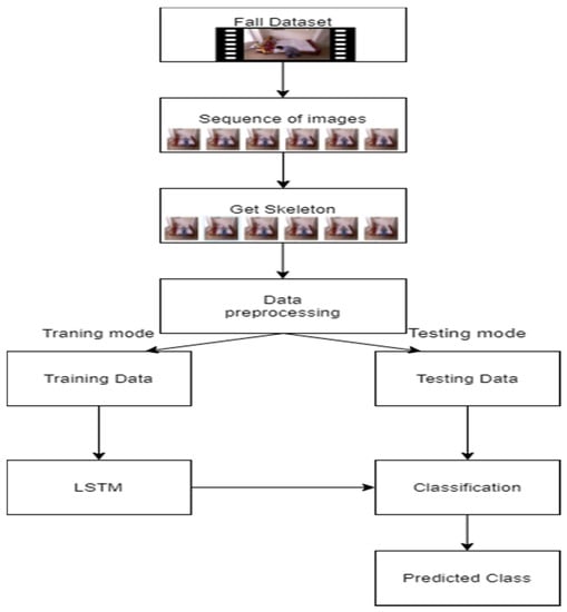
Figure 1.
Block diagram of the proposed fall detection framework process.
2.1. Data Set
The UR Fall Detection Dataset is produced by the Interdisciplinary Center for Computational Modeling of Rzeszow University. The content contains 70 (30 falls and 40 activities of daily living) sequences at a rate of 30 frames per second. Both fall events and other daily living activities such as standing, squatting down to pick up objects, and lying down were recorded. The environment has sufficient lighting. Two Microsoft Kinect cameras were used to record the fall event with the corresponding accelerometer data. The fall events were recorded with two cameras, and only one camera and an accelerometer were used for recording daily activities. As shown in Figure 2a, the height of the device is around the waist of a human body, and the image size is 640 × 480. We group these image sequences into a group of 100, and after data enhancement, there are 792 groups in total.
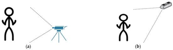
Figure 2.
Dataset device location. (a) UR Fall Detection Dataset device location; (b) Fall Detection Dataset device location.
For the Fall Detection Dataset presented in [23,24], data were recorded in five different rooms from eight different viewing angles. There were five participants in this study, including two males and three females. The activities the participants were instructed to perform include standing, sitting, lying down, bending and crawling, and they were recorded at a rate of 30 pictures per second. As shown in Figure 2b, the height of the device position is about 45 degrees of elevation of the human body′s line of sight. The original image size is 320 × 240, the adjusted image size is 640 × 480, the image sequence is a group of 100, and after data enhancement, there is a total of 936 groups.
We mixed these two datasets, on the one hand to ensure a sufficient amount of data, on the other hand to increase sample diversity to avoid overfitting. As shown in Table 1, we extracted the same amount of fall and non-fall events data from each dataset, respectively, to form a Mix Dataset in this study for model training.

Table 1.
The dataset composition.
2.2. OpenPose to Retrieve Human Skeleton
OpenPose is a supervised convolutional neural network based on Caffe for real-time multi-person 2D pose estimation developed by Carnegie Mellon University (CMU) [25]. It can realize posture estimation of human body movements, facial expressions, and finger movements. It is suitable for single- and multiple-user settings with excellent recognition effect and fast recognition speed.
The OpenPose algorithm calculates the human skeleton through Part Affinity Fields (PAFs) and Confidence Map. First, the feature map is obtained through the VGG-19 model. Then, the two-branch multi-stage CNN network is used to input the previously calculated feature map. The first branch is a set of 2D Confidence Maps for predicting joint parts, and the second branch is PAFs, which are used to predict limb parts. Finally, the confidence map and PAFs are analyzed through a greedy algorithm to generate 2D skeletons for the characters in the figure.
As shown in Figure 3, there are 25 joint points in the human body estimated by OpenPose, with Point 0 indicating the nose, 15~18, the right and left eyes and ears, 1, the neck, 2~7, the right and left shoulders, elbows and wrists, 8, the center of the hip, 9~14, the right and left hips, knees and ankles, and 19~24, the left and right soles, toes and heels.
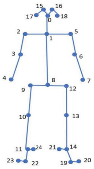
Figure 3.
Human skeleton joint points (25 points).
Figure 4 shows the joint points captured by OpenPose. It can be seen that this method can identify the joint points of a human body in a complex environment, especially in a dark ambient environment, as shown in Figure 4b. An matrix is generated for each frame, which includes the (x, y) coordinates of the 25 joint points and the prediction score of the joint point. The higher the score, the higher the accuracy of the joint point position.
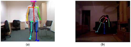
Figure 4.
Joint points captured by OpenPose. (a) Bright ambient light; (b) Dim ambient light.
2.3. Data Pre-Processing
Pre-processing of data is a very important part, because the data initially acquired may not have the same format or unit. Therefore, it is necessary to adjust the format, remove outliers, fill in missing values, or scale features. The following subsections explain the processes for data format adjustment, data normalization, and missing values recovery.
2.3.1. Format Adjustment
The original matrix becomes an matrix after removing the joint point scores. There are 100 pictures in one group, a total of 1140 groups. The input of a recurrent neural network needs to be a one-dimensional matrix. The matrix is then converted to a as input.
2.3.2. Relative Position Normalization (RP-Normalization)
In order to improve the accuracy of the model, we use the min-max normalization [26,27,28] to scale the data to the interval [0, 1] to improve the convergence speed of the model. The new scale data are defined as
where is the original data, is the minimum value in the data, and is the maximum value in the data.
However, there are missing points in the dataset. The value of 0 means that will be 0, but not all groups have missing values. Therefore, the original data distribution will be changed, resulting in unclear and complicated features. Therefore, we propose a normalization method to move the original coordinate position to the relative coordinate positions of the f-th frame as
and
respectively. Here, and H denote the width and the height of the picture, respectively. When or is equal to 0, it is regarded as a missing point and not calculated. If the center point is a missing point, it will be directly replaced by the calculated center point.
The distances () that need to be displaced are defined as
and
respectively, where the 8th joint point is () and the central hip circumference is used as the reference point, and the displacement is to the center point (,). When the displacement value is less than 0, it means a move to the right, and when the displacement value is greater than 0, it means a move to the left.
The new joint point coordinates () for calculating the displacement to the relative position are defined as
and
respectively, where the original joint point coordinate is () and the required displacement distance is ().
There are two advantages to this. The first is to avoid calculating the missing points together, and the original data distribution will not be affected. The second is to reduce unnecessary features. Because the objective of this study is fall detection, it removes the original data. The characteristics of the human body displacement process, such as walking from left to right or walking from far to near, fix the human skeleton in the same position, and make continuous movements to make the model easier to learn.
As shown in Figure 5, we unify the image size to 640 × 480 pixel and set a center point. After displacement by the above formula, as shown in Figure 6, the human skeleton will be moved to the center of the image and the central hip joint point will be equal to the center point position. In the skeleton diagram of fall and non-fall activities, we found that some joint points are not important for the recognition of fall events, so we remove them. Too many feature parameters may also cause the recognition rate to decrease or complicate the environment. Only 15 important points are retained as training feature values, among which the joint points of nose, shoulders, elbows, wrists, neck, hip, knees and ankles are retained.
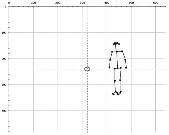
Figure 5.
The position and number of the original human skeleton coordinates.
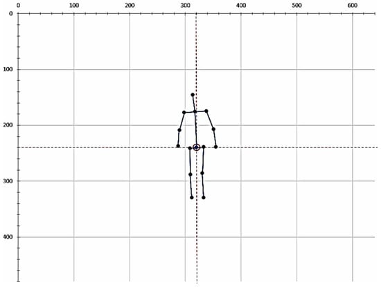
Figure 6.
The position and number of joint points after displacement.
2.3.3. Compensation for Missing Value
OpenPose still uses 2D image features to obtain the skeleton, so when these features are missing, problems such as unpredictability or prediction errors will occur. As shown in Figure 7, when the human body is overlapped, obscured, the outline of the human body is not clear, or the upper and lower feet of the human body appear, it will cause loss and errors when generating the skeleton. In this paper, we use a linear interpolation method to compensate for the missing values. We set 100 pictures as a group and use the original non-missing value data to interpolate missing data in the following pictures to ensure that there is enough data.
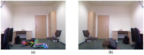
Figure 7.
Missing joint points. (a) The arm is obscured by the body, resulting in the loss of wrist joints; (b) Because the front and back features of the 2D image are not clear, Part Affinity Fields (PAFs) and Confidence Map cannot calculate the human skeleton.
The interpolation method can estimate the subsequent data value through the original data. If the original number of the joint points is too few, the error of the calculated missing value to its actual value will be large. Linear interpolation uses two known data points and calculate the slope of the two point. The estimated value Y is defined as:
where and are known data in the dataset, and is any data between and . Linear interpolation is fast and simple, but the accuracy is not high. In this paper, we set a threshold such that if the original joint points () are missing more than 67%, no compensation will be performed.
As an example, Figure 8 shows the y coordinates of a hand joint point of 30 consecutive pictures while a person makes a gesture of raising and lowering the hand. The first 15 pictures are gradually raising the hand, and the hand is lowered from the 16th picture. We use these data to evaluate the error between the compensated values and the original values.
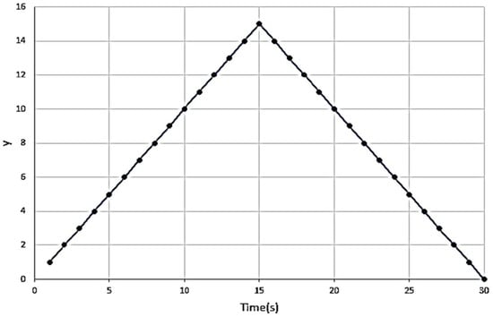
Figure 8.
The hand y point changes.
Figure 9 shows when the turning point is not a missing point, there will be no excessive error between the estimated value and the actual value. As shown in Table 2, the original dataset has a total of 2,850,000 joint points, and the missing points are 520,112. After normalization, there are 15 joints left. The original dataset has 1,710,000 with 214,707 missing points. The number of joint points after missing value compensation is the same as that after normalization, while the number of missing points is reduced to 27,849. Among them, the missing joint points of the original dataset accounted for 18.2%. After regularization, 10 unimportant joint points were removed, and the missing joint points accounted for 12.5%. After the missing value compensation, the missing joint points accounted for 1.6%. The reduction in missing points can help the model to reduce noise and increase accuracy during training.
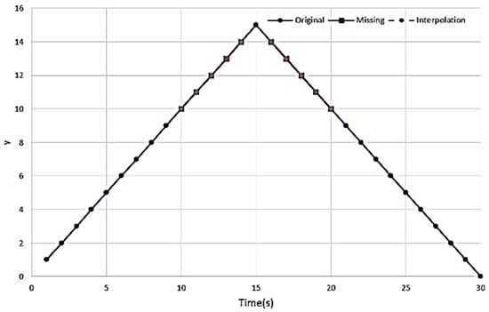
Figure 9.
Linear interpolation compensates for missing points (points 10–14, points 16–20 are missing).
Table 2.
Proportion of missing points.
2.4. Model Architecture
We chose RNN, LSTM and GRU models to learn with the joint points with time characteristics, because the RNN is suitable for dealing with problems that are highly related to time series. At the same time, it does not need to be calculated as a full image detection method, as using the entire picture increases training time and hardware burden. Moreover, the human joints are connected, so the posture will have a certain rule in the change of time t.
2.4.1. Recurrent Neural Network (RNN)
RNN [29,30] can describe dynamic behavior, as shown in Figure 10. Unlike the feedforward neural network (FNN) that accepts more specific structure input, RNN transmits the state in its own network cyclically, so it can accept a wider range of time series structure input.
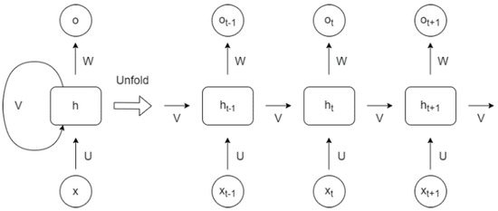
Figure 10.
Recurrent Neural Network (RNN) [29].
The difference between RNN and FNN is that RNN can pass the calculated output of the layer back to the layer as input, and o is the output vector. The two are defined as [29]
and
respectively. Here, t is time, h is the vector of the hidden layer, x is the input vector, V, W, and U are the parameter weights, b is the partial weight, and and are both excitation functions.
2.4.2. LSTM
LSTM is the evolution of RNN and was first proposed by S. Hochreiter and J. Schmidhuber (1997) [31]. It is often used in speech recognition [32], stock price prediction [33] and pedestrian trajectory [34]. LSTM improves the problem of RNN long-term memory and adds the concept of cell state. As shown in Figure 11, LSTM adds four structures, including forgetting gate, cell state, input gate and output gate, to keep the important features.
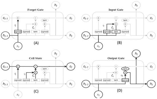
Figure 11.
Long short-term memory (LSTM) [31]. (A) Forget Gate; (B) Input Gate; (C) Cell State; (D) Output Gate.
The main core of LSTM is the cell state. By designing a structure called gate, LSTM has the ability to delete or add information to the cell. The forgetting gate can determine the information that needs to be discarded in the cell state, which is defined as [31]
where the lowercase variable is a vector, the matrix is the input weight, the matrix is the weight of the cyclic connection, is the partial weight, and the subscript f is for Forget Gate. Similarly, the subscript of information of Input Gate, Output Gate and Cell State can be expressed by i, o, and c, respectively. t is the time, h is the output vector, and is the Sigmoid function. Observe Forget Gate’s activation vector is used to determine whether to retain this information.
Knowing what new information will enter the cell are the input gate , and the activation vector for the new candidate value , which are defined as [31]
and
respectively, where is the tanh function.
Cell renewal is calculated through , is the cell state vector, , which is the activation vector of the output gate, and , the current output vector. They are defined in [32] as
and
respectively, where ⊙ represents the Hadamard product.
2.4.3. Gated Recurrent Unit (GRU)
GRU [35,36] is a gating mechanism for recurrent neural networks, introduced by Kyunghyun Cho et al. in 2014 [37], in order to improve the slower execution speed of LSTM, to speed up execution and reduce memory consumption. At the same time, it has a pretty good performance in a huge dataset. As shown in Figure 12, GRU replaces the Forget Gate and Input Gate in the LSTM with an Update Gate and changes the Cell State and Hidden State () to Merging, so it has fewer parameters than LSTM.
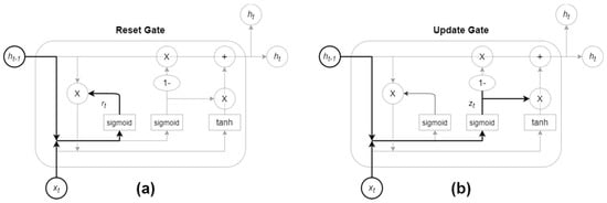
Figure 12.
Gated recurrent unit (GRU): (a) Reset Gate; (b) Update Gate [36].
The principle behind GRU is very similar to LSTM, using the Gate mechanism to control input, memory and other information. The GRU has two gates, one is the Reset Gate and the other is the Update Gate. Resetting the gate will determine that the new input information is combined with the memory at time t − 1. Here, z is the vector of the update gate defined as [36]
where W and U are the weight parameters, b is the partial weight, and is the Sigmoid function.
The Update Gate defines the amount of time (t − 1) memory saved to the current time t, r is the Reset Gate vector, h is the output vector, and the retained characteristic value is passed to the next time. They are defined as [36]
and
respectively.
As shown in Figure 13, in order to set 30 inputs, respectively, the (x, y) coordinates of 15 joint points are input as feature values. One hidden layer was set up for RNN, LSTM, and GRU. Since the recurrent neural network is more complex than other neural networks such as ANN, there is no need for too many hidden layers, otherwise the model will be too complicated. The Softmax layer is added, which normalizes the output of multiple neurons to (0, 1) interval. For example, in the end, two categories will have two scores with 0.7 and 0.3, and the Softmax layer will output the highest score value and complete the classification.
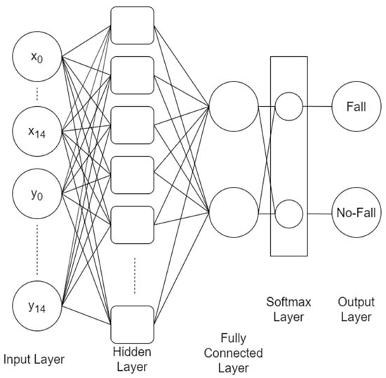
Figure 13.
Fall down model architecture.
2.5. Experiment Environment
The neural network model is trained on the Google Colaboratory platform [38], using CPU and GPU for training, and the software environment is Keras 2.3.1, as shown in Table 3. We use three different models, namely RNN, LSTM, and GRU for experiments and compare their performance in fall detection.
Table 3.
Model training parameters.
For training, we randomly divide 1140 groups of mixed datasets into 80% training set and 20% test set, resulting in 916 training sets and 224 test sets. The training sets are set up in batches and invested a number of training data to learn in each set. This study sets 916 to the same size as the training set. The reason for this is that the model can find the gradient to the best value faster. However, if there are more data or the hardware is slower, insufficient memory problems may occur. We also evaluated the performance under different Learning Rate (LR), which is the step size to find the best value. If LR is too large, the best value will not be found, and the training speed will be too small.
Table 4 shows the parameters for the training model. There are four datasets, which include the original dataset, the one with minimum and maximum normalization, the one with relative position normalization, and the one with linear interpolation plus relative position. According to the different datasets, we set 50 and 30 inputs, which are the original 25 joint points and the (x, y) coordinates of 15 joint points, respectively, as the feature value input. There are 64 to 1024 hidden neurons in the hidden layer. Because different datasets require different hidden layers and the number of hidden neurons, we evaluated a different range of numbers to find the best choice. Because there are missing points, it is necessary to use the excitation function whose output is centered at 0, so that when the input is 0, the output is also 0.
Table 4.
Model structure parameters.
3. Model Evaluation and Results
3.1. Loss Function
Loss function, also known as the Object function, is used to calculate the gap between the predicted value of the neural network and the target value. The smaller the loss function, the better the accuracy of the neural network. Cross Entropy, which is a loss function that describes the size of the difference between the model′s predicted value and the real value, is often used in classification problems. Suppose is a real event, is the probability of an event, the loss function is defined as [29]
where is the size of the test set, and is the classification category.
3.2. Model Evaluation Index
Accuracy, Precision, and Recall are common evaluation indicators for classification [39]. As shown in Figure 14, a confusion matrix is used to calculate the evaluation index to detect the performance of the classification model.
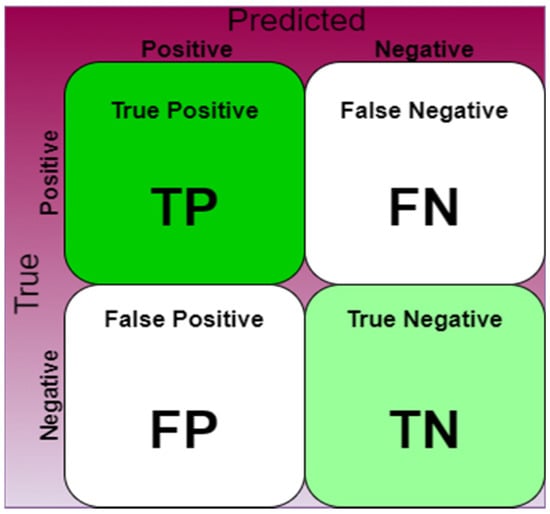
Figure 14.
Confusion Matrix [36].
Here, positive is the target of the main classification, negative is the target of the secondary classification, and True and False are the correct and wrong results, respectively. These are divided into four prediction situations: (True Positive (TP)), (True Negative (TN)), (False Positive (FP)) and (False Negative (FN)). TP is the main target of correct prediction, TN is the secondary target of correct prediction, FP is the main target of wrong prediction, and FN is the secondary target of wrong prediction.
3.2.1. Sensitivity
Sensitivity refers to the proportion of all samples that are actually the main classification target (positive), which is predicted to be the main classification target. If the true event is a fall (positive), the model predicts a fall as well. Sensitivity is defined as the ratio of the two
3.2.2. Specificity
Specificity refers to the proportion of all samples that are actually secondary classification targets (negative) judged to be secondary classification targets. If the true event is non-fall (negative), the model prediction is also non-fall, and the ratio of the two is
3.2.3. Accuracy
Accuracy refers to the proportion of the primary and secondary classification targets that are correctly judged in all classified samples. Like all events, the model correctly predicts the proportion of falls and non-falls.
3.3. RNN, LSTM and GRU Model Training Comparison
3.3.1. Comparison of Normalization Methods
This section compares different normalization methods, including No-Normalization, Min–Max Normalization, RP-Normalization, and linear interpolation plus RP-Normalization methods. In this study, we set hidden neurons to 64, learning rate 0.01, and observation dataset training and verification curves.
Figure 15 shows the RNN training and verification loss. As shown in Figure 15a, the maximum and minimum convergence speed is the fastest as it converges at Epochs 350 compared to others. The convergence speed refers to the time to reach the minimum error. Figure 15b shows the verification loss. Although the maximum and minimum convergences faster than other methods, there are many large fluctuations between Epochs 100 and 300. The reason for this is that the dataset is divided into missing values and non-missing values, which causes the data distribution change, thus increasing the uncertainty in training.
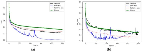
Figure 15.
RNN model training and verification loss. (a) Training loss; (b) Verification loss.
For RNN model, because its structure is simple, it can convergence fast for the dataset in a small value interval, and the method of normalization, relative position and linear interpolation plus relative position is not used. The dataset is a picture where the size is interval, so the convergence speed is slow. The improvement method can be adjusted from the structure and parameters.
Figure 16 shows the training and verification loss for LSTM. Figure 16a is the training loss. The structure of LSTM improves the long-term memory compared to RNN, so it has better performance. The relative position normalization method converges at Epochs 50, while for linear interpolation and the relative position method, convergence is at Epochs 250, and the loss error is reduced to less than 0.25. For the maximum and minimum, the training loss jumps up at Epochs 420. The reason for this is also that the training data distribution is damaged. Figure 16b is the verification loss. It shows that the proposed method using linear interpolation suffers from over-fitting because the structure or learning parameters are inappropriate.
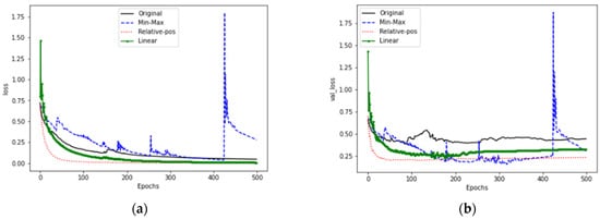
Figure 16.
LSTM model training and verification loss. (a) Training loss; (b) Verification loss.
Figure 17 shows the training and verification losses for GRU. Figure 17a is the training loss. Except for the maximum and minimum methods, the other three methods have lower error loss. The relative position normalization is the fastest to converge at Epochs 50. Figure 17b is the verification stage. The relative position normalization is the best, and the verification error loss is the smallest and the most stable. After adding linear interpolation, there is an over-fitting problem, so this article considers the structure, or the training parameters are inappropriate.
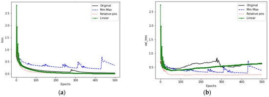
Figure 17.
GRU model training and verification loss. (a) Training loss; (b) Verification loss.
3.3.2. Hidden Nodes Comparison
This section examines the impact of different Hidden Nodes on the relative position normalization dataset. There are 64, 128, 256, 512 and 1024 different numbers, and the learning rate is 0.01. If there are too few Nodes, the problem may not be described. When there are more Nodes, a smaller error can be observed, but the convergence is slower. However, if the number of Nodes is continuously increased, the calculation time will increase, and smaller errors may not be found.
As shown in Table 5, we can see that the accuracy of 1024 Nodes is 88% for RNN. Because of the simple structure, more Nodes are needed to improve learning performance. However, 1024 Nodes are less effective for LSTM, with an accuracy of 94.6%. In fact, LSTM reaches the highest accuracy of 98.3% at 512. We hypothesize that this may be due to the complex structure of the LSTM model, and when too many Nodes are used it may over-describe the event, thus causing a decrease in accuracy. We observe the same trend for GRU and LSTM. The highest accuracy of GRU is 96.6% with 512 Nodes.
Table 5.
Model accuracy vs. number of nodes.
3.3.3. Learning Rate Comparison
This section chooses linear interpolation plus relative position and relative position data sets for comparison, because there is a slight overfitting problem in Loss during the training and verification stages. In this paper, we test when the neuron is 512 under the learning rate of 0.1, 0.01 and 0.001 to find the most suitable learning parameters.
From Table 6, we can see that RNN has the highest accuracy of 89% when LR = 0.1, while LSTM and GRU achieve higher accuracy when LR = 0.01. The accuracy is 98.3% and 96.6%, respectively.
Table 6.
Comparison of average accuracy of model learning rate (RP).
From Table 7, we can see that all three models achieve the highest accuracy when the learning rate is 0.1. The accuracy is 88.63%, 93.6%, and 96.3%, respectively. It is observed that the accuracy has not improved after interpolation, which may indicate that interpolation method does not have the correct compensation effect for the missing values.
Table 7.
Comparison of average accuracy of model learning rate (RP + Linear Interpolation).
3.4. RNN, LSTM and GRU Model Evaluation Indicators
This section discusses the evaluation indicators of the confusion matrix of the three models of each normalization method to evaluate the effectiveness of the model. The structure and parameters of the model used in the above subsections are used to obtain higher accuracy structures and parameters. The unnormalized, min–max normalization, and relative positions use 512 hidden Nodes and a learning rate of 0.01. Here, in linear interpolation we used the learning rate of 0.1.
Table 8 shows the sensitivity, specificity and accuracy of RNN for the no-normalization, min–max normalization, RP-normalization and linear interpolation+RP-normalization methods, respectively. Here, a higher sensitivity indicates a more accurate estimation of fall events. Accuracy indicates that the model correctly classifies fall and non-fall events, and the higher the accuracy, the greater the number of correctly classified events. This shows that the overall accuracy of the RNN model is up to 90.1%, using relative position plus linear interpolation. Although the specificity is increased, the sensitivity is reduced, and the highest sensitivity is the relative position normalization method.
Table 8.
Comparison of evaluation indicators of RNN model normalization methods.
Table 9 shows the above indicators for LSTM. It shows that the overall effect of using the maximum and minimum values is lower than that of unnormalized. The relative position method shows higher sensitivity and specificity, and lower error, than other methods when linear interpolation compensation is used. The effect of applying linear interpolation does not seem to be able to significantly improve the accuracy.
Table 9.
Comparison of evaluation indicators of LSTM model normalization methods.
Table 10 shows the above indicators for GRU. The GRU model has looser feature selection conditions due to reduced structure. Therefore, in the unnormalized dataset, it does not have the same accuracy as LSTM, but after using relative position normalization, the specificity is obvious increased from 76.7% to 98.2%, representing the classification accuracy of non-fall events. The overall accuracy has increased from 85.2% to 97.3%. Although the accuracy of GRU is not as high as LSTM, the specificity is higher than that of the other three models.
Table 10.
Comparison of evaluation indicators of GRU model normalization methods.
4. Discussion
This paper uses linear interpolation to compensate for the missing points. The experimental results show that the accuracy has not increased significantly. As shown in Figure 18, the missing point compensation is not as smooth as expected. Because there are nodes that change direction, we call it the turning point. For example, lifting the hand up is an inertial motion, so its direction can be predicted, but it is difficult to estimate when you will reach the highest point or how long you will stay at the highest point. It is shown that the part circled in red in the figure is the turning point of the action, from which the point starts to change direction. Figure 18a shows that the turning point is missing, but the y points of the sequence 14 and 16 are not lost. The distance is relatively close, so the error is less than or equal to 1. In Figure 18b, the y points of the sequence 10 to 20 are missing, including the turning point. Using the 9 and 21 points of the sequence to calculate the compensation value, we can see that the error is quite large, because the exact position of the turning point is not known and the interpolation calculation encounters a large error, where the maximum error is 5. In the case of a lost turning point, the maximum error is the lost turning point minus the compensation turning point.
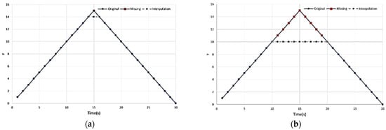
Figure 18.
Linear interpolation to compensate for missing points. (a) Point 15 (turning point) is missing; (b) Points 11–19 (including turning points) are missing.
Because the turning point cannot be estimated correctly. It causes wrong compensation when compensating for missing values, leading to features being eliminated or complicated. The inability of the model to learn effectively is the reason the accuracy cannot be further improved.
5. Conclusions
This paper proposes a fall detection framework using OpenPose to extract human skeleton from captured frames and recurrent neural network, long short-term memory and gated recurrent unit to detect fall based on skeleton data. Due to the correlation of the human skeleton, we believe that the change trajectory of the joint points is related to the human movement. This method has been shown to work well in a complex space environment with lower equipment costs. However, the joint points will be lost in some postures and actions, causing the model to have coagulation during training. Therefore, we will move the joint points to the set relative position and interpolate part of the data to improve the excessive noise and unnormalized happening. Recursive neural networks can effectively help learn the time changes in human joint points and reduce training time. Therefore, this paper proposes a fall detection model that learns the changes in human joint points in continuous time. The experimental results show that the fall detection accuracy of the proposed model is 98.2%, which outperforms the baseline 88.9%.
Author Contributions
Conceptualization, C.-B.L. and Y.-F.H.; methodology, C.-B.L. and Y.-F.H.; software, W.-K.K.; validation, C.-B.L., W.-K.K. and Y.-F.H.; formal analysis, C.-B.L. and Y.-F.H.; investigation, C.-B.L. and Y.-F.H.; resources, C.-B.L. and Y.-F.H.; data curation, C.-B.L. and W.-K.K.; writing—original draft preparation, W.-K.K. and Y.-F.H.; writing—review and editing, C.-B.L., and Z.D.; visualization, Z.D.; supervision, C.-B.L.; project administration, C.-B.L.; funding acquisition, C.-B.L. All authors have read and agreed to the published version of the manuscript.
Funding
This research was funded by the Ministry of Science and Technology in Taiwan under Grant No.: MOST 108-2637-E-324-004.
Institutional Review Board Statement
Not applicable.
Informed Consent Statement
Not applicable.
Data Availability Statement
Not applicable.
Conflicts of Interest
The authors declare no conflict of interest.
References
- National Development Commission, Population Estimates of the Republic of China (2018–2065). National Development Commission, 2018; pp. 1-1–2-11. Available online: https://www.ndc.gov.tw/en/Content_List.aspx?n=2A13C59DC7ABF742 (accessed on 9 March 2020).
- United Nations, Department of Economic and Social Affairs, Population Division. World Population Prospects 2019: Highlights, (ST/ESA/SER.A/423); United Nations, Department of Economic and Social Affairs: New York, NY, USA, 2019. [Google Scholar]
- United Nations, Department of Economic and Social Affairs. World Population Prospects the 2015 Revision, (ESA/P/WP.241); United Nations, Department of Economic and Social Affairs: New York, NY, USA, 2015. [Google Scholar]
- National Health Administration, Ministry of Health and Welfare. Available online: https://www.hpa.gov.tw/Pages/Detail.aspx?nodeid=807&pid=4326 (accessed on 9 March 2020).
- World Health Organization. Available online: https://www.who.int/zh/news-room/fact-sheets/detail/falls (accessed on 9 March 2020).
- Bahureksa, B.; Najafi, A.; Saleh, M.; Sabbagh, D.; Coon, M.; Mohler, J.; Schwenk, M. The Impact of Mild Cognitive Impairment on Gait and Balance: A Systematic Review and Meta-Analysis of Studies Using Instrumented Assessment. Gerontology 2017, 63, 67–83. [Google Scholar] [CrossRef] [PubMed]
- Romeo, L.; Marani, R.; Lorusso, N.; Angelillo, M.T.; Cicirelli, G. Vision-based Assessment of Balance Control in Elderly People. In Proceedings of the 2020 IEEE International Symposium on Medical Measurements and Applications (MeMeA), Bari, Italy, 1–3 July 2020; pp. 1–6. [Google Scholar]
- Romeo, L.; Marani, R.; Petitti, A.; Milella, A.; D’Orazio, T.; Cicirelli, G. Image-Based Mobility Assessment in Elderly People from Low-Cost Systems of Cameras: A Skeletal Dataset for Experimental Evaluations. In Proceedings of the 2020 International Conference on Ad-Hoc Networks and Wireless, ADHOC-NOW 2020, Ad-Hoc, Mobile, and Wireless Networks, Bari, Italy, 19–20 October 2020; Lecture Notes in Computer Science. Volume 12338, pp. 125–130. [Google Scholar]
- Lie, W.; Le, A.T.; Lin, G. Human Fall-Down Event Detection Based on 2D Skeletons and Deep Learning Approach. In Proceedings of the 2018 International Workshop on Advanced Image Technology (IWAIT), Chiang Mai, Thailand, 7–10 January 2018; pp. 1–4. [Google Scholar]
- Stone, E.E.; Skubic, M. Fall Detection in Homes of Older Adults Using the Microsoft Kinect. IEEE J. Biomed. Health Inf. 2015, 19, 290–301. [Google Scholar] [CrossRef] [PubMed]
- Nho, Y.; Lim, J.G.; Kwon, D. Cluster-Analysis-Based User-Adaptive Fall Detection Using Fusion of Heart Rate Sensor and Accelerometer in a Wearable Device. IEEE Access 2020, 8, 40389–40401. [Google Scholar] [CrossRef]
- Hussain, F.; Hussain, F.; Ehatisham-ul-Haq, M.; Azam, M.A. Activity-Aware Fall Detection and Recognition Based on Wearable Sensors. IEEE Sens. J. 2019, 19, 4528–4536. [Google Scholar] [CrossRef]
- Nguyen, T.; Cho, M.; Lee, T. Automatic Fall Detection Using Wearable Biomedical Signal Measurement Terminal. In Proceedings of the Annual International Conference of the IEEE Engineering in Medicine and Biology Society, Minneapolis, MN, USA, 2–6 September 2009; pp. 5203–5206. [Google Scholar]
- Taramasco, C.; Rodenas, T.; Martinez, F.; Fuentes, P.; Munoz, R.; Olivares, R.; De Albuquerque, V.C.; Demongeot, J. A Novel Monitoring System for Fall Detection in Older People. IEEE Access 2018, 6, 43563–43574. [Google Scholar] [CrossRef]
- Clemente, J.; Li, F.; Valero, M.; Song, W. Smart Seismic Sensing for Indoor Fall Detection, Location, and Notification. IEEE J. Biomed. Health Inf. 2020, 24, 524–532. [Google Scholar] [CrossRef] [PubMed]
- Ogawa, Y.; Naito, K. Fall Detection Scheme Based on Temperature Distribution with IR Array Sensor. In Proceedings of the IEEE International Conference on Consumer Electronics (ICCE), Las Vegas, NV, USA, 9–11 November 2020; pp. 1–5. [Google Scholar]
- Lin, B.; Su, J.; Chen, H.; Jan, C.Y. A Fall Detection System Based on Human Body Silhouette. In Proceedings of the 2013 Ninth International Conference on Intelligent Information Hiding and Multimedia Signal Processing, Beijing, China, 16–18 October 2013; pp. 49–52. [Google Scholar]
- Lin, C.; Wang, S.; Hong, J.; Kang, L.; Huang, C. Vision-Based Fall Detection through Shape Features. In Proceedings of the IEEE Second International Conference on Multimedia Big Data (BigMM), Taipei, Taiwan, 20–22 April 2016; pp. 237–240. [Google Scholar]
- Lotfi, A.; Albawendi, S.; Powell, H.; Appiah, K.; Langensiepen, C. Supporting Independent Living for Older Adults; Employing A Visual Based Fall Detection Through Analysing the Motion and Shape of the Human Body. IEEE Access 2018, 6, 70272–70282. [Google Scholar] [CrossRef]
- Gunadi, K.; Liliana; Tjitrokusmo, J. Fall Detection Application Using Kinect. In Proceedings of the International Conference on Soft Computing, Intelligent System and Information Technology (ICSIIT), Denpasar, Bali, Indonesia, 26–29 September 2017; pp. 279–282. [Google Scholar]
- Tsai, T.; Hsu, C. Implementation of Fall Detection System Based on 3D Skeleton for Deep Learning Technique. IEEE Access 2019, 7, 153049–153059. [Google Scholar] [CrossRef]
- Pishchulin, L.; Insafutdinov, E.; Tang, S.; Andres, B.; Andriluka, M.; Gehler, P.; Schiele, B. DeepCut: Joint Subset Partition and Labeling for Multi Person Pose Estimation. In Proceedings of the 2016 IEEE Conference on Computer Vision and Pattern Recognition (CVPR), Las Vegas, NV, USA, 27–30 June 2016; pp. 4929–4937. [Google Scholar]
- Kwolek, B.; Kepski, M. Human Fall Detection on Embedded Platform Using Depth Maps and Wireless Accelerometer. Comput. Methods Programs Biomed. 2014, 117, 489–501. [Google Scholar] [CrossRef] [PubMed]
- Adhikari, K.; Bouchachia, H.; Nait-Charif, H. Activity Recognition for Indoor Fall Detection Using Convolutional Neural Network. In Proceedings of the 2017 Fifteenth IAPR International Conference on Machine Vision Applications (MVA), Nagoya, Japan, 8–12 May 2017; pp. 81–84. [Google Scholar]
- Cao, Z.; Simon, T.; Wei, S.; Sheikh, Y. Realtime multi-person 2D Pose Estimation Using Part Affinity Fields. In Proceedings of the IEEE Conference on Computer Vision and Pattern Recognition (CVPR), Honolulu, HI, USA, 21–26 July 2017; pp. 1302–1310. [Google Scholar]
- Farooq, M.; Sazonov, E. Detection of Chewing from Piezoelectric Film Sensor Signals Using Ensemble Classifiers. In Proceedings of the 2016 38th Annual International Conference of the IEEE Engineering in Medicine and Biology Society (EMBC), Orlando, FL, USA, 20 August 2016; pp. 4929–4932. [Google Scholar]
- Wu, B.; Li, K.; Yang, M.; Lee, C. A Reverberation-Time-Aware Approach to Speech Dereverberation Based on Deep Neural Networks. IEEE/Acm Trans. Audiospeechlang. Process. 2017, 25, 102–111. [Google Scholar] [CrossRef]
- Sao, S.; Sornlertlamvanich, V. Long Short-Term Memory for Bed Position Classification. In Proceedings of the 2019 4th International Conference on Information Technology (InCIT), Bangkok, Thailand, 24–25 October 2019; pp. 28–31. [Google Scholar]
- Mikolov, T.; Karafiát, M.; Burget, L.; Cernocký, J.; Khudanpur, S. Recurrent Neural Network Based Language Model. In Proceedings of the Eleventh Annual Conference of the International Speech Communication Association, Chiba, Japan, 26–30 September 2010; pp. 2877–2880. [Google Scholar]
- Jun, K.; Lee, D.; Lee, K.; Lee, S.; Kim, M.S. Feature Extraction Using an RNN Autoencoder for Skeleton-Based Abnormal Gait Recognition. IEEE Access 2020, 8, 19196–19207. [Google Scholar] [CrossRef]
- Hochreiter, S.; Schmidhuber, J. Long Short-Term Memory. Neural Comput. 1997, 9, 1735–1780. [Google Scholar] [CrossRef] [PubMed]
- Billa, J. Dropout Approaches for LSTM Based Speech Recognition Systems. In Proceedings of the IEEE International Conference on Acoustics, Speech and Signal Processing (ICASSP), Calgary, AB, Canada, 15–20 April 2018; pp. 5879–5883. [Google Scholar]
- Wei, D. Prediction of Stock Price Based on LSTM Neural Network. In Proceedings of the 2019 International Conference on Artificial Intelligence and Advanced Manufacturing (AIAM), Dublin, Ireland, 16–18 October 2019; pp. 544–547. [Google Scholar]
- Xue, H.; Huynh, D.Q.; Reynolds, M. SS-LSTM: A Hierarchical LSTM Model for Pedestrian Trajectory Prediction. In Proceedings of the 2018 IEEE Winter Conference on Applications of Computer Vision (WACV), Lake Tahoe, NV, USA, 12–15 March 2018; pp. 1186–1194. [Google Scholar]
- Fu, R.; Zhang, Z.; Li, L. Using LSTM and GRU Neural Network Methods for Traffic Flow Prediction. In Proceedings of the 2016 31st Youth Academic Annual Conference of Chinese Association of Automation (YAC), Wuhan, China, 11–13 November 2016; pp. 324–328. [Google Scholar]
- Pavithra, M.; Saruladha, K.; Sathyabama, K. GRU Based Deep Learning Model for Prognosis Prediction of Disease Progression. In Proceedings of the 2019 3rd International Conference on Computing Methodologies and Communication (ICCMC), Erode, India, 27–29 March 2019; pp. 840–844. [Google Scholar]
- Cho, K.; van Merriënboer, B.; Gulcehre, C.; Bougares, F.; Schwenk, H.; Bengio, Y. Learning Phrase Representations using RNN Encoder-Decoder for Statistical Machine Translation. In Proceedings of the 2014 Conference on Empirical Methods on Natural Language Processing (EMNLP), Bengio, Yoshua, 29 October 2014; pp. 1724–1734. [Google Scholar]
- Google, Colaboratory. Available online: https://research.google.com/colaboratory/faq.html (accessed on 7 September 2020).
- Huang, H. Available online: https://medium.com/@chih.sheng.huang821/ (accessed on 22 March 2020).


Publisher’s Note: MDPI stays neutral with regard to jurisdictional claims in published maps and institutional affiliations. |
© 2020 by the authors. Licensee MDPI, Basel, Switzerland. This article is an open access article distributed under the terms and conditions of the Creative Commons Attribution (CC BY) license (http://creativecommons.org/licenses/by/4.0/).