Development of a Throughflow-Based Simulation Tool for Preliminary Compressor Design Considering Blade Geometry in Gas Turbine Engine

Abstract

Gas turbine engines are highly intricate machines, and every component of them is closely associated with one another. In the traditional engine developing process, vast experiment tests are needed. To reduce unnecessary trials, a whole gas turbine engine simulation is extremely needed. For this purpose, a compressor simulation tool is now developed. Considering the inherent drawbacks of 0D analysis and 3D CFD (Computational Fluid Dynamics) calculation, the 2D throughflow method is an indispensable tool. Based on the circumferential average method (CAM), 3D Navier–Stokes is transformed into a 2D method. One phenomenon arising is that the lack of description about circumferential motion leads to the need for the blade force modeling in compressor simulation. Previous models are based on the assumption that flow passes through the average stream surface without entropy increasing, which is not applicable in the CAM. An improved model is proposed based on the result analysis from CAM and NUMECA method in a linear cascade. Whereafter, the model is applied in a highly loaded and low-speed fan, which has been tested for its performance characteristics. Utilizing the new model, the error of the adiabatic efficiency between CAM and experiment decreases from 4.0% to 1.0% and the accuracy of the mass flow, and pressure ratio remains unchanged. The time involved in the CAM simulation is nearly 70 times faster than that of the 3D simulation.

1. Introduction

When a new gas turbine engine is under development, abundant hardware builds are necessary to measure the performance characteristics, which are much too expensive [1]. Therefore, the simulation of an overall gas turbine engine is extremely needed. Thanks to both the advance of the CFD (Computational Fluid Dynamics) and the increasingly developed computer technology, fully three-dimensional (3D) computation is increasingly involved [2,3]. However, it is very time-demanding. For example, when Medic et al. [4] simulated a $20°$ sector gas turbine engine (shown as Figure 1) on the coarse grids containing 14 million cells, a simulation was performed in nearly 2 weeks relying on 700 processors [5,6,7,8]. On the other hand, the zero-dimensional method (0D) commonly used in the performance evaluation cannot present the radial distribution of aerodynamic parameters. Therefore, the throughflow method (2D) is still a significant part of its performance prediction and rapid flow field acquisition [9]. To achieve this ultimate goal of the whole gas turbine engine simulation, the throughflow method applied in compressors is first explored in this paper.

The most widely used throughflow method is the streamline curvature method. Comparing with it, the circumferential average method (CAM) first, proposed by Smith [10] is appealing in the following aspects: choke mass flow can be predicted, certain types of shock can be captured, and the same code can be used for subsonic, transonic and supersonic meridional velocities. Much research has been performed based on the CAM in turbomachinery. However, one element indispensably mentioned in every throughflow method applied in turbomachinery is that the absence of the description about the circumferential motion leads to the blade force missing (shown as Figure 2), which needs the blade force modeling appended. As for the inviscid blade force model, it was first presented by Baralon [11]. In his method, the blade force modeling was proposed based on the fully time-dependent axisymmetric Euler equations. In this theory, the flow conformed to the average stream surface for each blade row, and the blade force must be orthogonal to the average stream surface in order to obtain a loss-free flow turning. Moreover, the blade force, which they thought determined the flow path, was its tangential component. Based on the theory of Baralon, Simon [12] modified the calculation formula of the inviscid blade force, where the tangential component of the inviscid blade force was substituted by the modulus of the inviscid blade force in the calculation formula. For the design mode of turbomachinery, it was first proposed by Sturmayr and Hirsch [13], where the target tangential velocity was prescribed through the flow angle at the trailing edge (TE). In their research, how the circumferential velocity evolves inside the blade passage in the streamwise direction is needed to be given. Dawes [14] adopted another method in the solution of the inviscid blade force, where the blade force was computed from the circumferential momentum and was not solved anymore in the bladed regions. The aforesaid methods depended on a formulation, which had a constant coefficient determining the convergence effect. Based on these methods above, convergence problems often arose when iteratively solving these inviscid blade force formulations, especially with an inappropriate relaxation factor. Considering this, Jin [15] presented a method similar to the large-particle method to avoid solving the inviscid blade force explicitly. This method consisted of two steps for each time step. First, the effects caused by the inviscid blade force in the momentum equations were neglected. Moreover, then only the effects caused by the inviscid blade force were taken into account in the governing equations. However, all these foregoing methods are dependent on the assumption of the average stream surface. Moreover, the average stream surface is calculated through the mean camber surface with the deviation angle. That is, when the flow passes through the average stream surface, the inviscid blade force is to deflect the flow, and no entropy increasing occurs. Therefore, it requires that the inviscid blade force be normal to the average stream surface. However, this assumption is not applicable in the CAM, which needs to take into consideration the effect of the blade geometry on the inviscid blade force. In this paper, the modeling of the inviscid blade force considering the effect of the blade geometry is discussed and verified.

This paper focuses on two parts of the CAM derived from the Navier–Stokes (N-S) equation. The first part is about the deduction of the inviscid blade force concerning the blade geometry from the equation and its modeling process. The second part is about the application of this modeling. It is successively applied in the throughflow simulation of a subsonic linear cascade, a transonic linear cascade. All these results are compared with 3D simulation results. Finally, it is involved in the simulation of a highly loaded and low-speed fan named TA36 and calculation results are compared with the experimental data as well as CFD results.

2. Materials and Methodologies

2.1. Throughflow Analysis Tool

In this research, the throughflow model used is the CAM to derive the governing equations. For the 3D flow in aviation turbomachinery, the CAM method applied for any parameter is defined as

$$\overline{q}\left(x,r,t\right)=\frac{1}{{\phi }_s-{\phi }_p}{\displaystyle {\int }_{{\phi }_p}^{{\phi }_s}q\left(x,r,\phi ,t\right)}d\phi$$

(1)

where $q$ is an aerodynamic parameter, $\overline{q}$ is the circumferential value, ${\phi }_s$ and ${\phi }_p$ are angular values for suction side and pressure side individually. In a vane passage shown in Figure 3, the integral equation starts from the suction side to the pressure side.

A blockage factor due to the circumferential blade thickness takes on the form:

$$b=\frac{{\phi }_s-{\phi }_p}{2\pi /N}$$

(2)

where $N$ is the number of blades.

After the definition of the CAM, aerodynamic parameters can be decomposed into circumferential average and spatial fluctuation:

$$q\left(x,r,\phi ,t\right)=\overline{q}\left(x,r,t\right)+q^{\prime }\left(x,r,\phi ,t\right)$$

(3)

Based on the CAM and the main operation rule, the N-S equation in the relative frame can be derived into:

$$\frac{\partial \overline{U}}{\partial t}+\frac{1}{br}\frac{\partial }{\partial x}\left[br\left(\overline{F}-\overline{F_v}\right)\right]+\frac{1}{br}\frac{\partial }{\partial r}\left[br\left(\overline{G}-\overline{G_v}\right)\right]=\overline{S}+F_B+F_F$$

(4)

where

$$\begin{gathered} \overline{U}=\left[\begin{array}{c}\overline{\rho }\\ \overline{\rho }\overline{\overline{w_x}}\\ \overline{\rho }\overline{\overline{w_r}}\\ \overline{\rho }\overline{\overline{w_u}}\\ \overline{\rho }\overline{\overline{e}}\end{array}\right],\overline{F}=\left[\begin{array}{c}\overline{\rho }\overline{\overline{w_x}}\\ \overline{\rho }\overline{\overline{w_x}}\overline{\overline{w_x}}+\overline{p}+\overline{\rho }\overline{\overline{{w^{″}}_x{w^{″}}_x}}\\ \overline{\rho }\overline{\overline{w_r}}\overline{\overline{w_x}}+\overline{\rho }\overline{\overline{{w^{″}}_r{w^{″}}_x}}\\ \overline{\rho }\overline{\overline{w_x}}\overline{\overline{w_u}}+\overline{\rho }\overline{\overline{{w^{″}}_x{w^{″}}_u}}\\ \overline{\rho }\overline{\overline{i}}\overline{\overline{w_x}}+\overline{\rho }\overline{\overline{i^{″}{w^{″}}_x}}\end{array}\right],\overline{G}=\left[\begin{array}{c}\overline{\rho }\overline{\overline{w_r}}\\ \overline{\rho }\overline{\overline{w_x}}\overline{\overline{w_r}}+\overline{\rho }\overline{\overline{{w^{″}}_x{w^{″}}_r}}\\ \overline{\rho }\overline{\overline{w_r}}\overline{\overline{w_r}}+\overline{p}+\overline{\rho }\overline{\overline{{w^{″}}_r{w^{″}}_r}}\\ \overline{\rho }\overline{\overline{w_u}}\overline{\overline{w_r}}+\overline{\rho }\overline{\overline{{w^{″}}_u{w^{″}}_r}}\\ \overline{\rho }\overline{\overline{i}}\overline{\overline{w_r}}+\overline{\rho }\overline{\overline{i^{″}{w^{″}}_r}}\end{array}\right], \\ \overline{F_v}=\left[\begin{array}{c}0\\ \overline{{\tau }_{xx}}\\ \overline{{\tau }_{xr}}\\ \overline{{\tau }_{ux}}\\ \overline{{\tau }_{xx}{w}_x}+\overline{{\tau }_{xr}{w}_r}+\overline{{\tau }_{ux}{w}_u}-\overline{q_x}\end{array}\right],\overline{G_v}=\left[\begin{array}{c}0\\ \overline{{\tau }_{xr}}\\ \overline{{\tau }_{rr}}\\ \overline{{\tau }_{ru}}\\ \overline{{\tau }_{xr}{w}_x}+\overline{{\tau }_{rr}{w}_r}+\overline{{\tau }_{ru}{w}_u}-\overline{q_r}\end{array}\right]\overline{S}=\left[\begin{array}{c}0\\ 0\\ \frac{\overline{\rho }{\left(\overline{\overline{w_u}}+\omega r\right)}^2+\overline{p}+\overline{\rho }\overline{\overline{{w^{″}}_u{w^{″}}_u}}-\overline{{\tau }_{uu}}}{r}\\ \frac{-\overline{\rho }\overline{\overline{w_r}}\left(\overline{\overline{w_u}}+2\omega r\right)-\overline{\rho }\overline{\overline{{w^{″}}_r{w^{″}}_u}}+\overline{{\tau }_{ru}}}{r}\\ \overline{\rho }\overline{\overline{w_r}}{\omega }^{2}r\end{array}\right], \\ {F}_B=\frac{N}{2\pi b}\left[\begin{array}{c}0\\ \left(p_s\frac{\partial {\phi }_s}{\partial x}-p_p\frac{\partial {\phi }_p}{\partial x}\right)\\ \left(p_s\frac{\partial {\phi }_s}{\partial r}-p_p\frac{\partial {\phi }_p}{\partial r}\right)\\ \frac{\left(p_p-p_s\right)}{r}\\ 0\end{array}\right],F_F=\frac{N}{2\pi br}\left[\begin{array}{c}0\\ {\left({\tau }_{bwx}\right)}_p+{\left({\tau }_{bwx}\right)}_s\\ {\left({\tau }_{bwr}\right)}_p+{\left({\tau }_{bwr}\right)}_s\\ {\left({\tau }_{bw\phi }\right)}_p+{\left({\tau }_{bw\phi }\right)}_s\\ 0\end{array}\right] \end{gathered}$$

where $U$ is the vector of conservative variables, $F$ and $G$ are the convective flux vectors, $F_v$ and $G_v$ are the viscous flux vectors, $S$ is the source term, $F_B$ is the inviscid blade force and $F_F$ is the viscous blade force. $\rho$ is density, $p$ is pressure; $w_x$, $w_r$,$w_u$ are scalar values for relative velocity in $x$, $r$ and $\phi$ direction, respectively; $e$ and $i$ are the relative total energy and total enthalpy per unit individually and they take on the form:

$$e=c_{v}T+\frac{1}{2}\left(w_x{}^2+w_r{}^2+w_u{}^2\right)$$

(5)

$$i=e+\frac{p}{\rho }$$

(6)

where $c_v$ is the specific heat at a constant volume.

In Equation (4), the first row represents the continuity equation, rows 2–4 depict the momentum equations, and the last row describes the energy balance. A time-marching finite volume method is used to solve the equation. The Edwards’ LDFSS [16] scheme is applied to discretize the convective fluxes. The calculation of the viscous fluxes requires the evaluation of the primitive variables and their first derivatives at the edge middle of the considered cell. The Green–Gauss theorem is also used to estimate the gradient of the variables. An explicit Runge–Kutta method is chosen for the time discretization as it is straightforward to implement. Meanwhile, local time step and implicit residue averaging are used to accelerate the convergence.

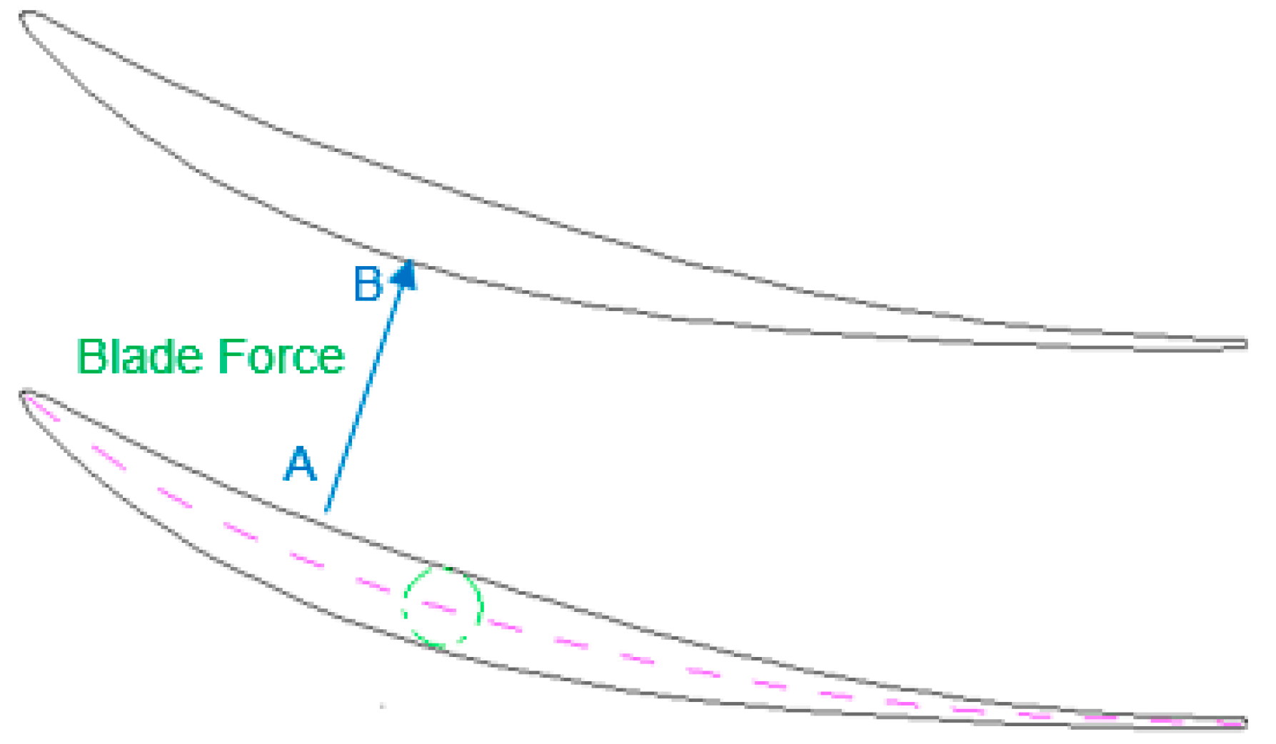
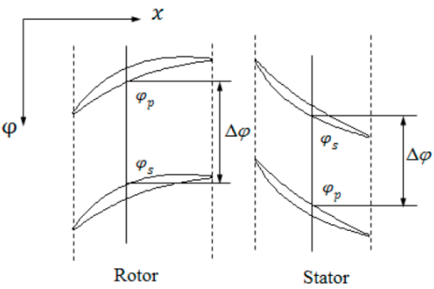
2.2. Development of the Inviscid Blade Force

In previous research, the inviscid blade force was usually modeled as a term related to time and then solved through the iteration method. The formula proposed by Sturmayr and Hirsch [17] is:

$$\frac{\partial \left(\rho f_{Bu}\right)}{\partial \tau }=C\rho \left(w_u{}^{\mathrm{target}}-w_u\right)$$

(7)

where $\tau$ is the pseudo time; $C$ is a constant value used in iteration to regulate the convergence of iteration; $w_u{}^{\mathrm{target}}$ is the target tangential velocity; $w_u$ is the tangential velocity determined in the throughflow method.

Based on this method, researchers make several improvements upon the inviscid blade force. For example, Simon [18] put forward a model

$$\frac{\partial \left(\rho f_B\right)}{\partial \tau }=-C\rho \left(w_x{n}_{Bx}+w_r{n}_{Br}+w_u{n}_{Bu}\right)$$

(8)

where $f_B$ is the magnitude of the inviscid blade force; $n_{Bx}$,$n_{Br}$ and $n_{Bu}$ are components of the unit normal vector of the average stream surface.

The modeling of all these inviscid blade force models is based on the assumption that the effect produced by the inviscid blade force is to change the flow direction without entropy production. Therefore, the direction of the inviscid blade force must be orthogonal to the average stream surface. However, these models do not take the effect of the blade geometry into consideration, which is not suitable in the CAM.

According to Formula (4), the inviscid blade force takes the form

$$F_B=\frac{N}{2\pi b}\left[\begin{array}{c}0\\ \left(p_s\frac{\partial {\phi }_s}{\partial x}-p_p\frac{\partial {\phi }_p}{\partial x}\right)\\ \left(p_s\frac{\partial {\phi }_s}{\partial r}-p_p\frac{\partial {\phi }_p}{\partial r}\right)\\ \frac{\left(p_p-p_s\right)}{r}\\ 0\end{array}\right]$$

(9)

Based on the coordinate definition of the mean camber surface:

$${\phi }_M={\phi }_M\left(x,r\right)$$

(10)

The circumferential coordinates of the suction side and the pressure side can be displayed as:

$$\begin{array}{l}{\phi }_s={\phi }_M+\frac{\pi }{N}\left(1+b\right)\\ {\phi }_p={\phi }_M+\frac{\pi }{N}\left(1-b\right)\end{array}$$

(11)

and ${\left(r\frac{\partial {\phi }_M}{\partial x},r\frac{\partial {\phi }_M}{\partial r},-1\right)}^T$ represents the normal vector of mean camber surface for a blade.

Therefore, the inviscid blade force can be transformed as:

$$F_B=\left[\begin{array}{c}0\\ \frac{N\left(p_s-p_p\right)}{2\pi b}\left(\frac{\partial {\phi }_M}{\partial x}\right)+\frac{p_s+p_p}{2}\frac{\partial b}{b\partial x}\\ \frac{N\left(p_s-p_p\right)}{2\pi b}\left(\frac{\partial {\phi }_M}{\partial r}\right)+\frac{p_s+p_p}{2}\frac{\partial b}{b\partial r}\\ \frac{N}{2\pi rb}\left(p_p-p_s\right)\\ 0\end{array}\right]$$

(12)

That is,

$$\begin{array}{l}{F}_{Bx}=\frac{N\left(p_s-p_p\right)}{2\pi b}\left(\frac{\partial {\phi }_M}{\partial x}\right)+\frac{p_s+p_p}{2}\frac{\partial b}{b\partial x}\\ F_{Br}=\frac{N\left(p_s-p_p\right)}{2\pi b}\left(\frac{\partial {\phi }_M}{\partial r}\right)+\frac{p_s+p_p}{2}\frac{\partial b}{b\partial r}\\ F_{Bu}=\frac{N\left(p_p-p_s\right)}{2\pi rb}\end{array}$$

(13)

It can be seen that the axial and the radial components of the inviscid blade force include two parts. First, the first item is related to the circumferential inviscid blade force, and it is easy to know:

$$\{\begin{array}{c}\tan {\gamma }_M=\frac{r\partial {\phi }_M}{\partial r}\\ \tan {\lambda }_M=\frac{r\partial {\phi }_M}{\partial x}\end{array}$$

(14)

where ${\gamma }_M$ and ${\lambda }_M$ are the axial flow angle and the radial flow angle, respectively, for the mean camber surface.

Therefore, the axial and radial components of the inviscid blade force can be transformed into:

$$\begin{array}{l}{F}_{Bx}=-F_{Bu}\tan {\lambda }_M+\frac{p_s+p_p}{2}\frac{\partial b}{b\partial x}\\ F_{Br}=-F_{Bu}\tan {\gamma }_M+\frac{p_s+p_p}{2}\frac{\partial b}{b\partial r}\end{array}$$

(15)

Through this formula, it is revealed that the axial and radial components of the inviscid blade force are not only related to the circumferential component of the inviscid blade force and the flow angle of the blade camber surface but also are concerned with the blockage factor and the static pressure on the blade surface. This aspect has not been concerned in the former models. When the thickness of the blade changes rapidly along the axial or the radial direction, the inviscid blade force is no longer normal to the mean camber surface. Given this, the second component needs more consideration. However, the first item can be calculated through the circumferential component of the inviscid blade force and flow angle, whereas the second item needs to be modeled. As this study is about the directive problem of turbomachinery, the partial derivative of the blockage factor along the axial and the radial direction can be calculated. However, the pressure on the suction and pressure side cannot be acquired in CAM, which needs to be modeled.

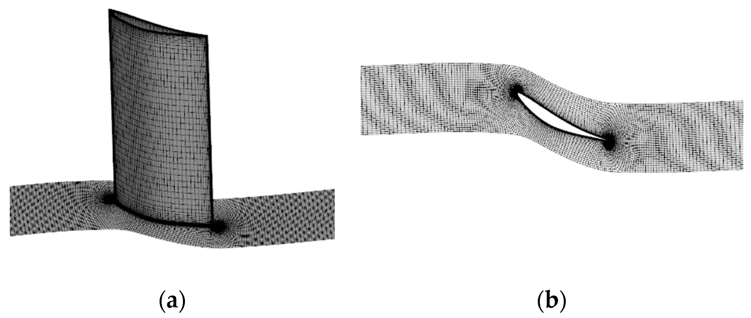
2.3. 3D CFD Method Verification

In this study, the analyses of the CAM results are based on the 3D simulation results. To perform the 3D simulation in this study, the commercial numerical software NUMECA was used to simulate the linear cascade and the TA36. The mesh generation for the calculation was completed by the IGG module of the NUMECA. The Fine module of the NUMECA is widely used to calculate the steady flow in turbomachinery. To validate the applicability of the 3D CFD method, the simulation of a controlled diffusion airfoil (CDA) linear cascade was carried out.

The experiment results of the linear cascade have been published in the works of Steinert [19]. In their papers, the coordinates of the blade geometry have been listed. Based on this, the calculation model was constructed. The H-O-H topology was adopted for the linear cascade to get a better mesh quality. After the grid independence check, the total number of grid points is nearly 7.1 × 10⁵, shown in Figure 4. Moreover, it is observed that the y+ is less than five after the calculation results are obtained. In this study, the Spalart–Allmaras (S–A) turbulence model was applied. At the inlet, the flow direction is axial, the total temperature is 288.15 K, and the total pressure is 101,325 Pa. At the outlet, the boundary condition is adjusted to make sure that the Mach number is the same as the experiment condition. No-slip condition is applied at the wall surface.

When the convergent results were acquired, the pressure distribution on the blade surface was compared with the experiment results, shown in Figure 5. From this figure, the distribution is nearly the same except for some points. Therefore, it can be reached that the NUMECA software is suitable to be applied in the further simulation of 3D models.

3. Modeling of the Inviscid Blade Force Based on a Linear Cascade

To investigate the inviscid blade force in the CAM, a simple linear cascade is involved. Based on this model, the other relevant factors which may influence the axial inviscid blade force can be excluded. Since no change occurs in the spanwise direction, the radial blade force $F_{Br}$ equals 0. A CDA linear cascade is applied in the study, and its geometry parameters are shown in

Table 1. Basic parameters of the linear cascade.

Parameters	Values
Chord	100 mm
Blade geometric inlet angle	$40°$
Stagger angle	$15.2°$
Aspect ratio of the cascade	6.0
Solidity	2.15

:

In this paper, when studying this model, Euler equations are adopted in the CAM, which means that viscous blade force and viscous stress are neglected. In the simulation of the 3D method, Euler equations are also involved, and they are solved using NUMECA. The boundary conditions for these two methods are the same. At the inlet, the flow direction is axial, the total temperature is 288.15 K, and the total pressure is 101,325 Pa. At the outlet, the mass flow is set to ensure the Mach number at the inlet. No-penetration condition is applied at the wall surface.

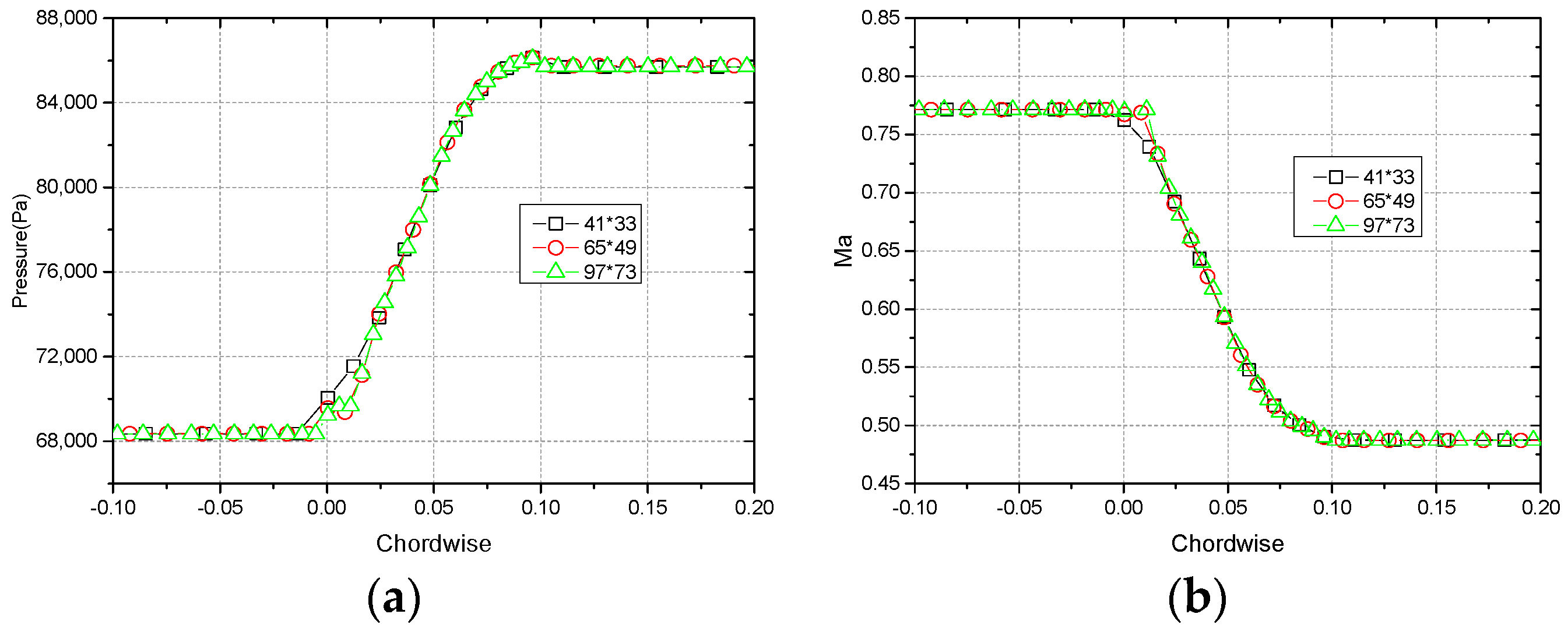
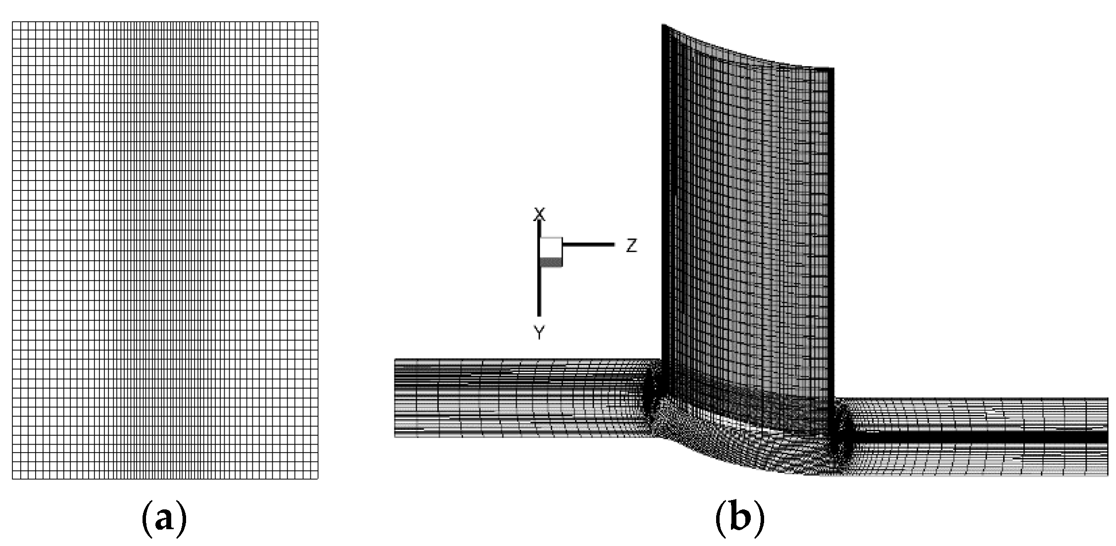
3.1. Grid Independence Verification

To prove the reliability of the calculation results, it is necessary to verify the grid independence before the study. In the CAM, three types of mesh with different numbers of grid points were generated to calculate the model. The topology of the mesh and the boundary conditions were set the same. Moreover, the grid numbers are 41 × 33, 65 × 49, 97 × 73 (axial direction radial direction), respectively. The linear cascade was simulated on the subsonic condition. Based on results from these three grids, the distribution of static pressure and the Mach number are shown in Figure 6. The curves of the case with 65 × 49 grid points coincide with that of the case with 97 × 73 grid points. Hence, in conclusion, when the number of grid points exceeds 65 × 49, the results are considered independent of the grid number. In consideration of the calculation accuracy and the requirement of saving time, the numerical method with 65 × 49 grid points was introduced into this study.

The grid number of 3D grids used in NUMECA is, respectively, 160k, 310k and 550k. The boundary conditions for the three grid topologies are the same. Moreover, the boundary conditions are the same as the one in the CAM method. Based on the results from these three grids, the distribution of static pressure on the blade surface and the total pressure at the outlet are shown in Figure 7. The curves of the case with 310k grid points coincide with that of the case with 550k grid points. Hence, in conclusion, when the number of grid points exceeds 310k, the results are considered independent of the grid number. In consideration of the calculation accuracy and the requirement of saving time, the numerical method with 310k grid points was involved in this study.

Therefore, grids for these two methods are displayed in Figure 8. The grid settings in CAM are 65 and 49 in the axial and radial direction, respectively. In the 3D method, the grid type is H-O-H, and the total grid number is 310k. The CAM needs a CPU time of 100 ss on a laptop, while the 3D calculation requires 2 h on 4 cores of an Intel Xeon E5-2650 [email protected] processor.

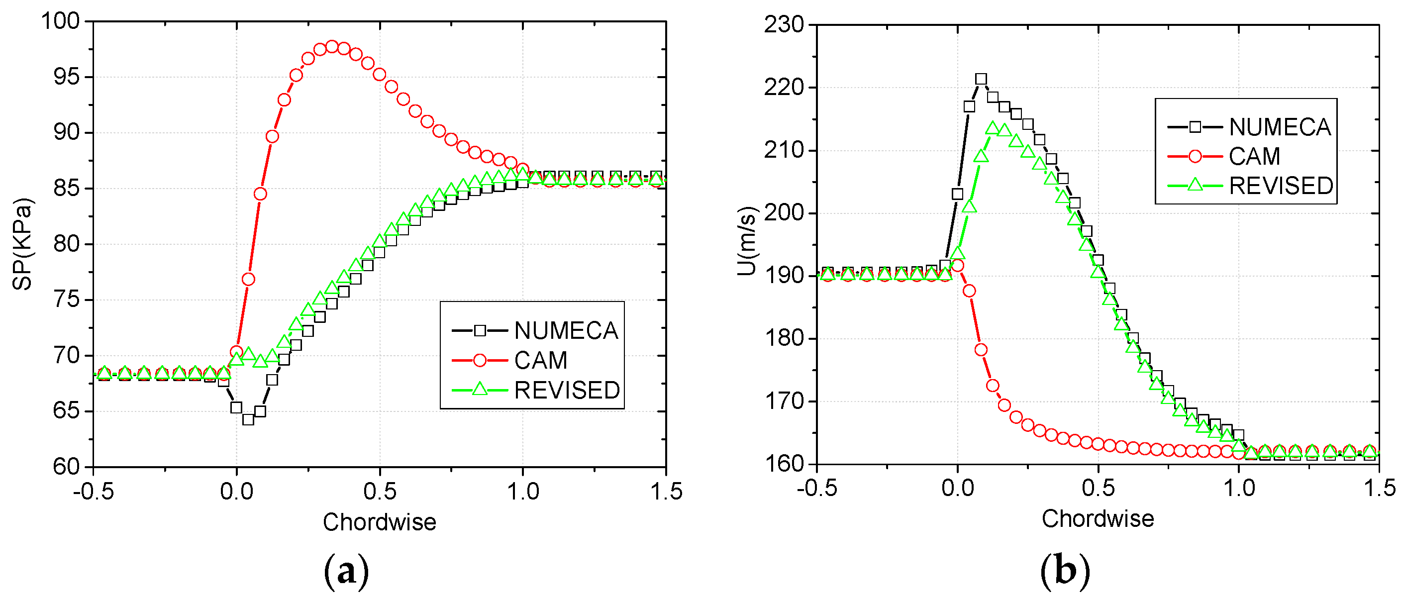
3.2. Model Analysis on the Subsonic Condition

First, a comparison of the subsonic flow in linear cascade is performed, where mass flow at the outlet is set to ensure the inlet Mach number of M = 0.77. Figure 9 and Figure 10 show the isolines of the pressure and the axial velocity for both methods, and the values marked on them are the absolute values. In these figures, the leading edge (LE) and the trailing edge correspond to the beginning and end of the colorful isolines. One thing worth noting is that the circumferential average results from the 3D results are circumferentially mass average except the pressure, and for the pressure, it is the circumferential area average. Through these figures, it reveals that although parameters at the inlet and outlet are consistent, contours in the internal passage are different. These differences cannot be observed in the total pressure recovery coefficient and the spanwise distribution of parameters. In Figure 9b, the pressure obtained through the 3D method increases slowly, which shows the diffusive process in the vane passage. However, in the CAM, pressure first increases rapidly and then decreases slowly, which is contradicting to real flow. The velocity contours are shown in Figure 10 also reveal the difference between these two methods. The flow passes the LE should accelerate first and then decelerate with diffusion. However, in the result of CAM, the axial velocity decreases as soon as it flows into the blade passage. Figure 11a,b show the distribution of average pressure and axial velocity at the middle span, which also reveals the aforesaid phenomenon.

Figure 12a,b shows the distribution of the tangential and the axial components of the inviscid blade force at the middle span obtained in these two methods. Through comparison, it shows that the tangential component of the inviscid blade force has the same trend, which is solved through iteration. Since the tangential component is relatively accurate, the circulation at the inlet and outlet can be guaranteed, which makes the performance parameters from CAM similar to 3D results. However, the axial component has a great difference. Therefore, it is essential to depict the influence of the blade geometry on the inviscid blade force.

In Formula (15), it is shown that pressures at the suction side and the pressure side are needed to depict the inviscid blade force modeling. However, pressure on the suction and pressure side cannot be acquired in the throughflow method; the term $\frac{p_s+p_p}{2}$ needs to be modeled. Figure 13 shows the pressure distribution in the middle span obtained from NUMECA. PP and PS refer to pressures on the pressure side and the suction side severally, and AP means the algebraic mean value of pressure at both sides, which is $\frac{p_s+p_p}{2}$. SP means the spatially averaged value from 3D simulation results. From these figures, it can be observed that the trend of AP and SP is nearly the same, especially at the middle and posterior portion of the blade. Moreover, the average spatial pressure from the 3D numerical method has the same meaning as the average pressure proposed in the CAM method. Therefore, it is appropriate to use the average pressure in the CAM method in place of the term $\frac{p_s+p_p}{2}$.

Therefore, Formula (15) turns to be:

$$\begin{array}{l}{F}_{Bx}=-F_{Bu}\tan {\lambda }_M+\overline{p}\frac{\partial b}{b\partial x}\\ F_{Br}=-F_{Bu}\tan {\gamma }_M+\overline{p}\frac{\partial b}{b\partial r}\end{array}$$

(16)

The improved inviscid blade force model is applied in the CAM, where the boundary conditions remain the same as before. The axial and tangential components of the inviscid blade force obtained through these three methods are shown in Figure 14a,b (“REVISED” means the improved CAM). Through these figures, it can be seen that the axial component from the CAM improves greatly, which is nearly the same as the results from the 3D simulation. Moreover, the tangential component improves at the same time due to the influence of the axial blade force.

Figure 15 displays the flow field inside the cascade obtained through the improved inviscid blade force modeling. Through these figures, it can be seen that the contours are similar to 3D simulation results. Figure 16a,b show the distribution of average pressure and average axial velocity at the middle span, which can reveal the effect resulting from the improved modeling. Based on the original inviscid blade force modeling, the maximum error of pressure along the streamwise direction between CAM and 3D method at the middle span is 30.9%. After using the improved model, the error decreases to 9.0%. As for the axial velocity, it drops from 21.0% to 7.5% after using this model. Moreover, these differences all appear at the leading edge of the blade. These errors can be explained as follows: this improved model is not suitable for all conditions. At the LE, pressure on the suction side and the pressure side is relevant to the incidence angle and changes drastically, which needs further modification due to the incidence angle.

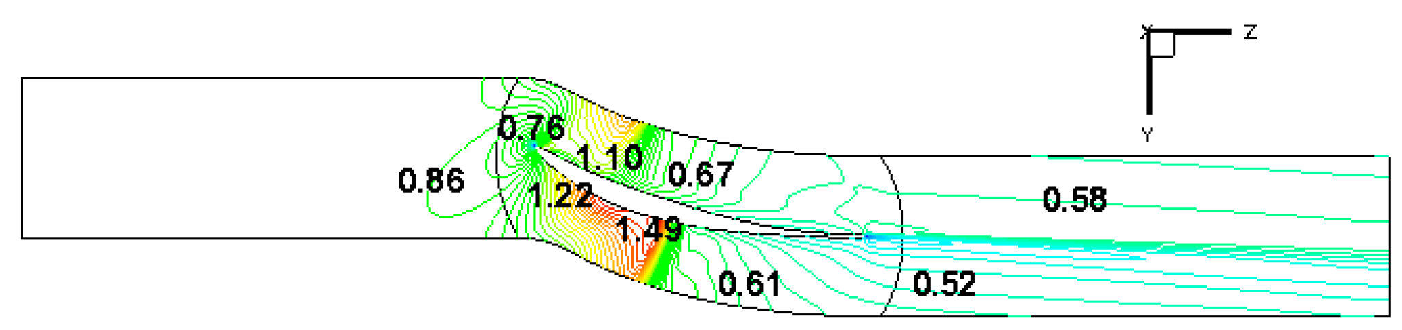
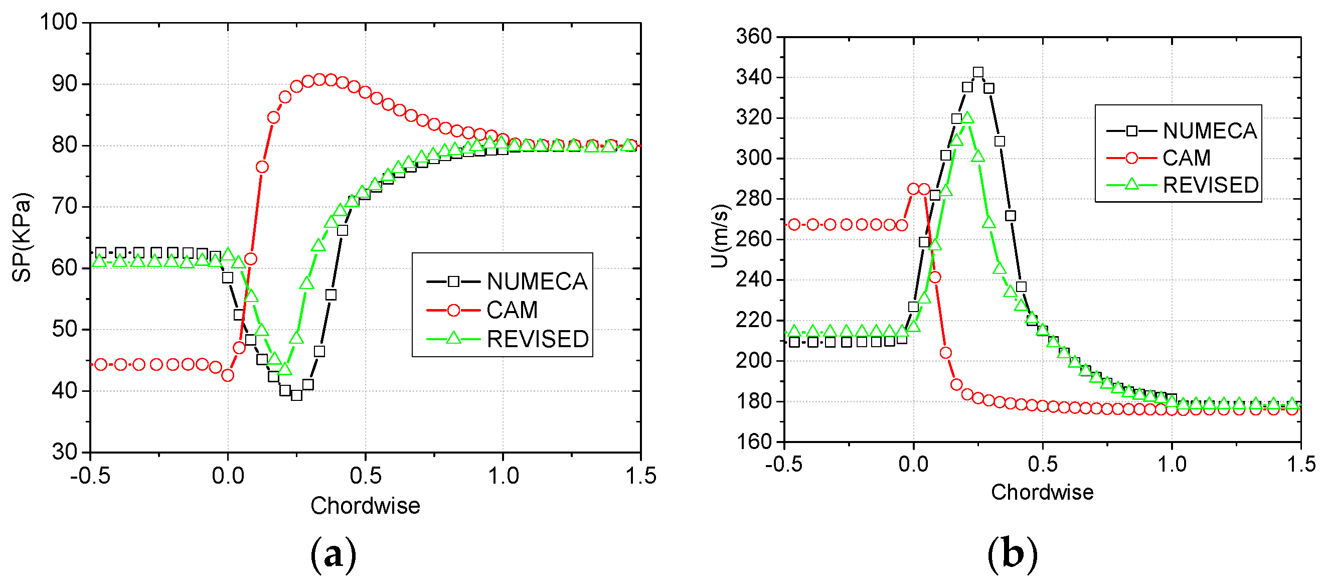
3.3. Model Analysis on the Transonic Condition

In previous research, when the CAM is applied in the transonic condition, a special shock wave was captured [13,17,20]. However, in real 3D transonic flow, the shock wave is normal to the blade geometry other than axisymmetric. Therefore, in the CAM, the shock wave should be eliminated, where a decelerating process exists. Considering this point, the inviscid blade force involved in the transonic cascade also needs to be improved.

First, a simulation of the transonic cascade is performed through the 3D method. By changing pressure at the outlet, the Mach number at the inlet is restricted to 0.86. The isoline of Mach numbers at the middle span is shown in Figure 17, which reveals that the strong shock wave exists on the suction side.

Similar to Figure 13, the distribution of pressure at the middle span is also displayed in Figure 18 for this condition. In this figure, it can be seen that the spatially averaged pressure from the 3D result is nearly the same as the algebraic mean value of the pressure side and the suction side. They have slight differences at the LE and the front half part, and its value at the shock wave of the suction side is a little different. However, they are coincident behind the shock wave.

To examine the influence of these two aforesaid inviscid blade force models on the result, they are both applied in the CAM simulation. The distribution of the pressure and the axial velocity at the midspan are compared in Figure 19. It reveals a huge difference between these two models. When the original inviscid blade force is used, the maximum error between CAM and 3D method for pressure along the flow direction is 128.1%, and it is 47.0% for axial velocity. However, when the improved model is used, these two values are reduced to 39.3% and 19.9%, respectively. The most obvious diversity exists at the position where shock wave occurs, and at other positions, these two sets of results obtained from the revised model and NUMECA are nearly the same. Finally, one element needs to be discussed. The maximum error of the static pressure is still 39.3%, which is still large. It is observed that the maximum error exists at the location of the shock. Considering the difficulties in the simulation of the shock with the throughflow method [11,13,20,21,22] and the improvement of the parameters in the blade passage, the method is regarded as an applicable method. To further improve the accuracy, there are two aspects that may need to consider. The first one is to add a factor in adjusting variable incidence angles, which makes this model more exact for different incidence angles. Moreover, the other one is that the circumferential fluctuation source terms [23,24] should also be considered in the governing equation since they also contribute to the flow structure.

4. Application of the Improved Inviscid Blade Force Model in a Highly Loaded Low-Speed Fan

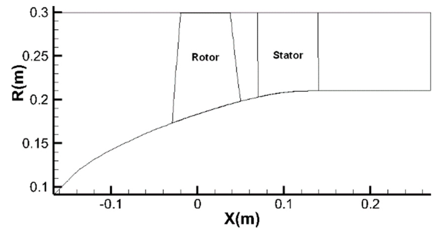
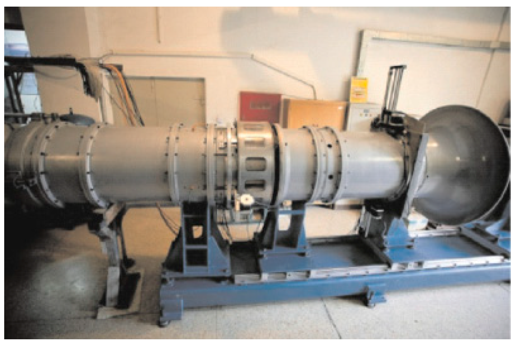
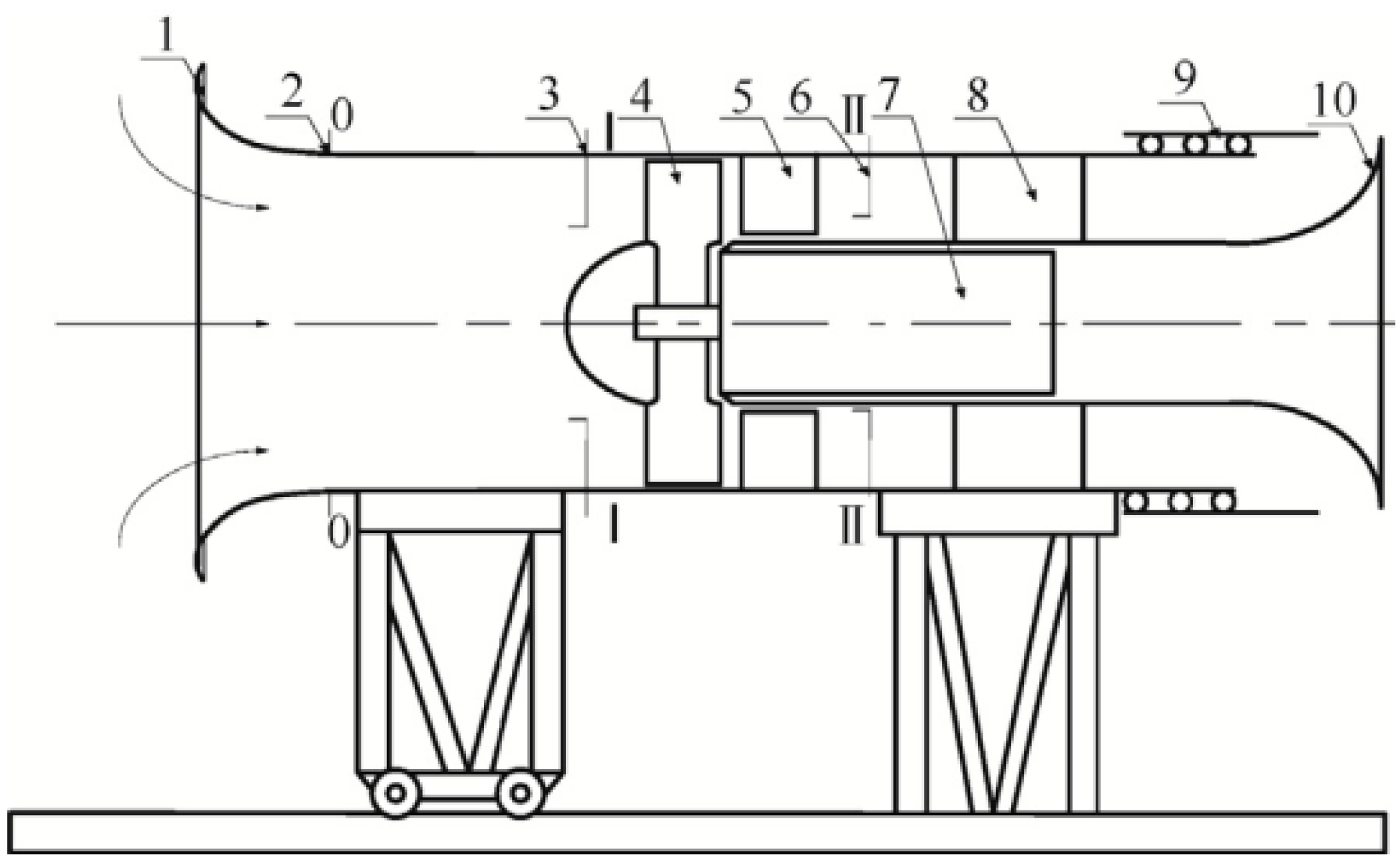
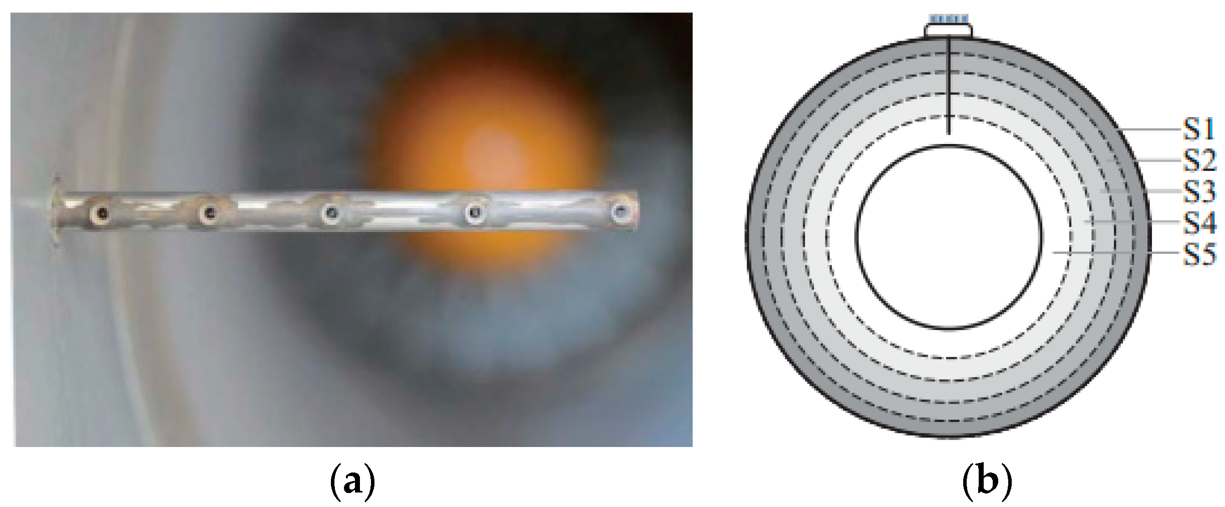
4.1. Experimental Facility

After the improved model of the inviscid blade, force is verified in the linear cascade; it is then applied in a fan named TA36 to validate its applicability. The TA36 is a highly loaded and low aspect ratio fan, which is comprised of a rotor and a stator. Moreover, the load coefficient is up to 0.258. The designed rotational speed is 2900 rpm. The flow path of the TA36 is displayed in Figure 20. The geometrical parameters of the TA36 are shown in

Table 2. Geometrical parameters of TA36.

Geometrical Parameter	Value
	Rotor	Stator
Number of blades	20	27
Tip diameter (mm)	600	600
Hub diameter (mm)	346	401
Stagger angle at the hub (°)	45	0
Aspect ratio	1.18	1.40

.

Figure 21 and Figure 22 display the test bench and the general schematic of the TA36. The meanings of location index in Figure 22 are as follows: 1-inlet flow tube, 2-measurement point of wall static pressure, 3-measurement point of inlet total pressure, 4-rotor, 5-stator, 6-measurement point of outlet total and static pressure, 7-motor, 8-brackets, 9-outlet adjusting components, 10-throttling valve. The rotor is motivated through an actuating motor, and the rotational speed of the rotor is controlled by a frequency transmitter. The working point of the fan is commanded by the opening degree of the throttle valve. The throttle valve consists of a fixed conical surface and a removable annular sleeve, which can modify the opening degree of the throttle valve by adjusting the relative position of these two components. The position of the annular sleeve is controlled by a stepping motor, which can make the fan work from the maximum mass flow point to the near stall point.

In this test facility, two planes named 3 and 6 are chosen to measure the total pressure at the inlet and the outlet of the fan. The total pressure is measured through the five-hole total pressure comb. The test instruments and their distribution are shown in Figure 23. The static wall pressure is measured at position 2 through four static pressure measuring holes, which are uniformly distributed in the circumferential direction. The static pressure sensor involved is Honeywell-0142PC01D. The steady-state pressure signal is delivered to the data acquisition board belonging to the NI PXI system through the terminal box. Through this method, the pressure parameters of the fan system are obtained. The torque of the actuating motor in the test is measured through the torque meter. With this approach, the rotational speed and torque can be obtained from the data acquisition system.

Before the measurement, the five-hole total pressure comb is calibrated. In order to guarantee the accuracy, repeated tests are conducted. The uncertainties of the mass flow rate and efficiency in this experiment are within 0.5%.

Next, the process of this experiment is described in detail. First, the area of the throttle valve is adjusted to the maximum, and the fan is accelerated to the set rotational speed. Then the opening area of the throttle valve is decreased slowly to make sure that the fan works at a quasi-steady state. With the fan working at the stall state, the throttle valve is opened to quit this stall state. In this experiment, the measurement parameters are the mass flow, total pressure ratio and efficiency. The volume flow rate of the fan is calculated as:

$$q_v=\alpha A_0\sqrt{\frac{2p_{sF}}{{\rho }_0}}$$

where $\alpha$ is the discharge coefficient of the fan, and it is 0.992 in the test, $A_0$ is the area of the inlet, ${\rho }_0$ is the density of the atmosphere, $p_{sF}$ is the pressure increase of the fan.

The efficiency formula is:

$$\eta =\frac{P_u}{P_a}$$

where $P_u$ is the useful power of the fan, and $P_a$ is the shaft power. They are defined as:

$$P_{in}=\sqrt{3}UI\cos \phi$$

where $U$ and $I$ are the voltage and the current of the motor, $\cos \phi$ is the power coefficient, whose range is 0.75–0.85.

$$P_a=q_v(p_{t2}-p_{t1})$$

where $p_{t1}$ and $p_{t2}$ are the total pressure at the inlet and outlet severally.

Therefore, the efficiency is calculated as:

$$\eta =\frac{q_v(p_{t2}-p_{t1})}{1000(\sqrt{3}UI\cos \phi ){\eta }_o{\eta }_a}$$

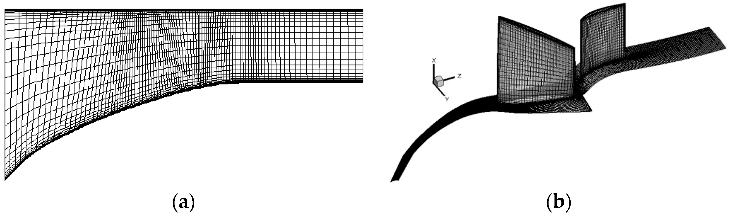
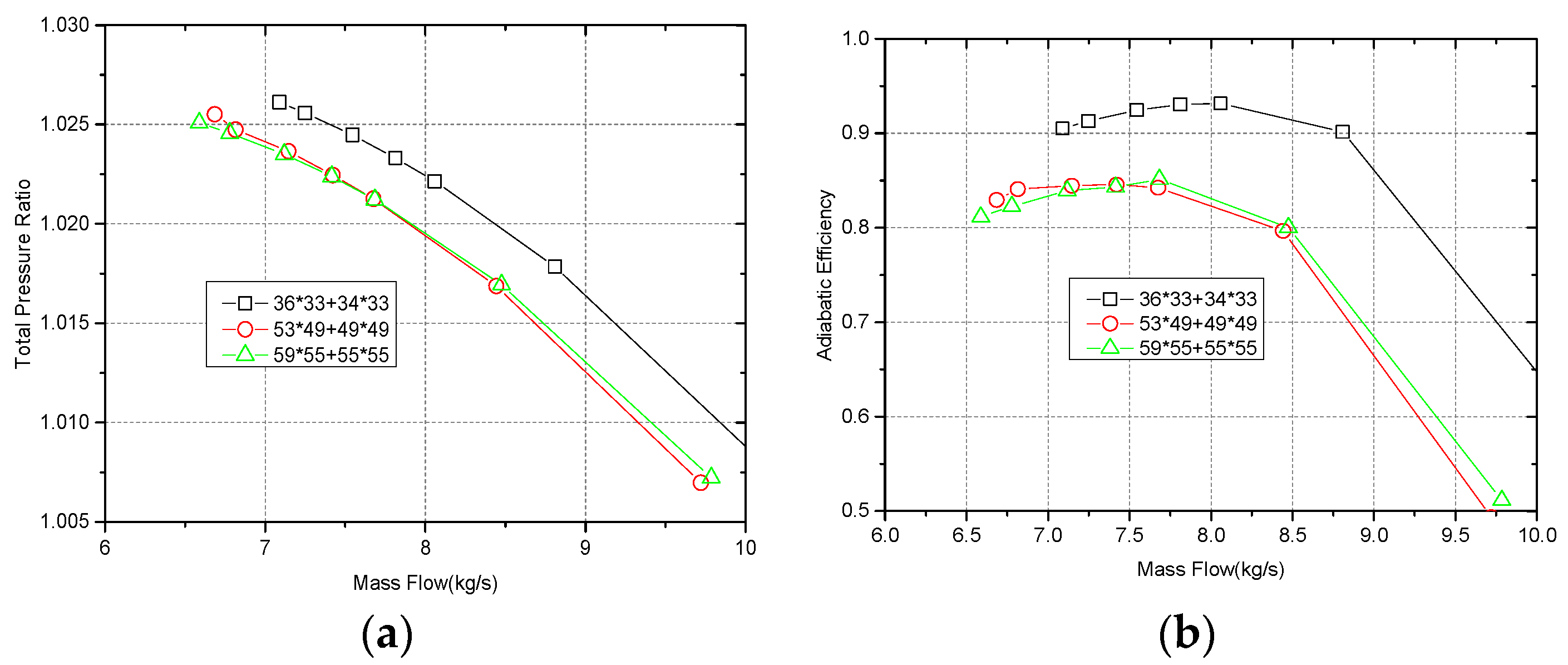
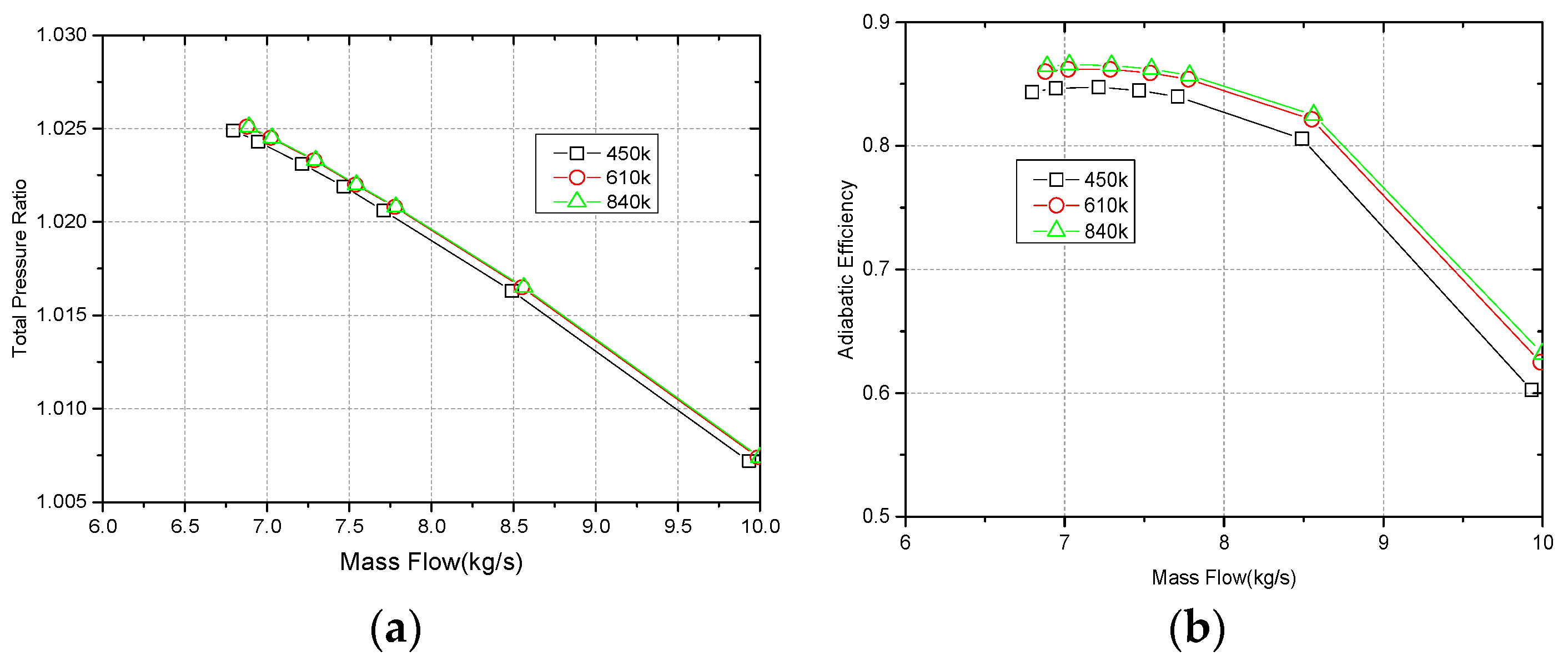
4.2. Grid Independence Verification

To verify the usability of the improved inviscid blade force model, the CAM based on N-S equations and the 3D method are both applied in the fan simulation. The computational grid topology used in both methods is shown in Figure 24.

The boundary condition for both simulations is set as follows: The total temperature and pressure are 288.15 K and 101,325 Pa severally. The inlet flow direction is axial. The pressure is restricted at the hub of the outlet, and the pressures at other positions of the outlet are obtained through a radial-equilibrium equation. At the solid wall, the no-slip boundary condition is used. The turbulence model is the S–A model.

To check the grid independence in the simulation of the TA36, three grids are made in both the CAM and NUMECA. For the CAM, the grid number is, respectively 36 × 33 + 34 × 33, 53 × 49 + 49 × 49, 59 × 55 + 55 × 55. The performance characteristics of this fan based on these three grids are obtained, shown in Figure 25. They are the pressure ratio versus the mass flow and the adiabatic efficiency versus the mass flow. The curves of the case with 53 × 49 + 49 × 49 grid points coincide with that of the case with 59 × 55 + 55 × 55 grid points. Hence, in conclusion, when the number of grid points exceeds 53 × 49 + 49 × 49, the results are considered independent of the grid number. In consideration of the calculation accuracy and the requirement of saving time, the numerical method with 53 × 49 + 49 × 49 grid points were involved in this study.

The grid number used in the NUMECA for the TA36 are, respectively, 450k, 610k, 830k. The performance characteristics of this fan based on these three grids are obtained, shown in Figure 26. They are the pressure ratio versus the mass flow and the adiabatic efficiency versus the mass flow. The curves of the case with 610k grid points coincide with that of the case with 830k grid points. Hence, in conclusion, when the number of grid points exceeds 610k, the results are considered independent of the grid number. In consideration of the calculation accuracy and the requirement of saving time, the numerical method with 610k grid points was introduced into this study.

Therefore, the mesh for the throughflow method is made of 53 × 49 (Rotor) + 49 × 49 (Stator) nodes. The computational region for the 3D method meshes with nearly 610,000 grids, and a tip clearance of 1 mm exists at the rotor domain.

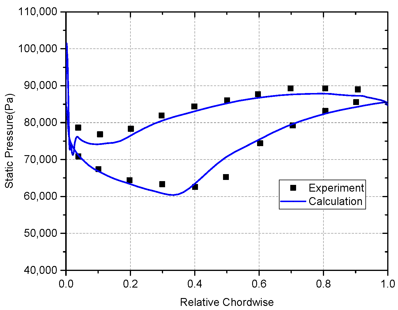
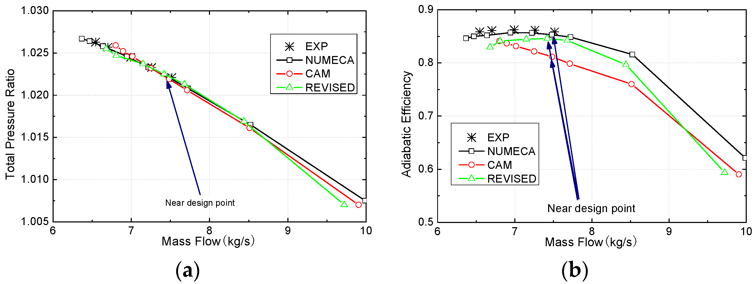
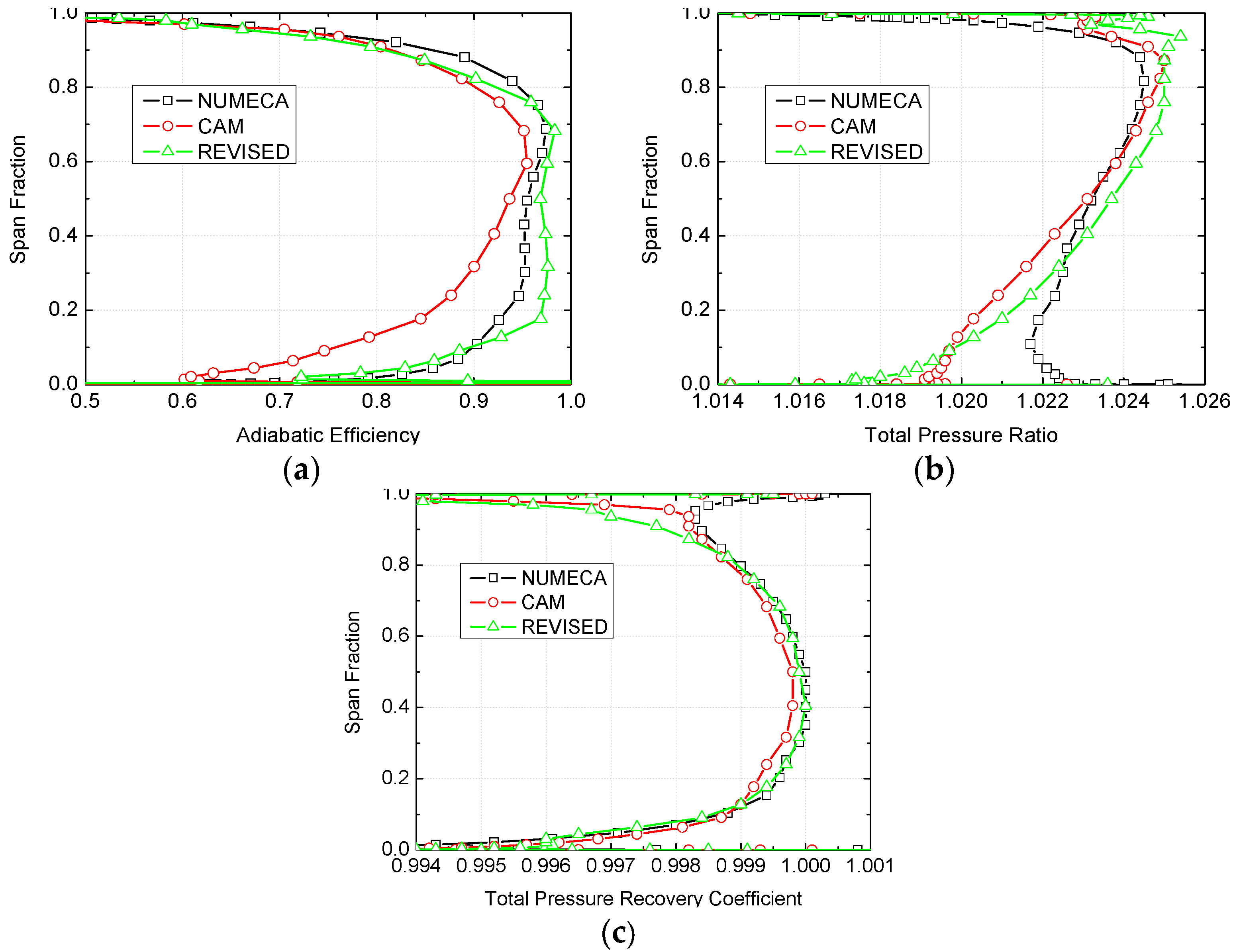
4.3. Numerical Analysis and Discussion

Figure 27a,b shows the overall characteristic lines acquired from the experiment, NUMECA and these two CAM methods. Figure 27a is shown for the characteristic of mass flow versus total pressure ratio. Figure 27b is for mass flow versus adiabatic efficiency. From these two figures, it is observed that the performance of efficiency is improved, and the characteristic of mass flow and pressure ratio remains unchanged.

The performance parameters on the design point acquired from different calculation methods are shown in

Table 3. Performance parameters of the TA36 near the design point.

	Mass Flow (kg/s)	Pressure Ratio	Adiabatic Efficiency	Power (kW)	Power Error (%)
Experiment	7.516	1.022	0.8583	15.81
NUMECA	7.480	1.022	0.8531	15.83	0.128
CAM	7.485	1.022	0.8113	16.66	5.357
Revised CAM	7.421	1.022	0.8457	15.84	0.207

. When the original inviscid blade force model is applied, mass flow and pressure ratio from CAM, experiment and 3D method is nearly the same. However, the error of adiabatic efficiency between them is more than 4.0%. This is related to the simulation accuracy of the flow field. The original model is based on the assumption that the inviscid blade force is perpendicular to the average stream surface, which leads to the wrong prediction of the field. While in fact, the inviscid blade force is not. After the improved inviscid blade force model is applied, the error of adiabatic efficiency between throughflow and experiment or 3D simulation is about 1%.

Figure 28a,c shows the distribution of rotor pressure ratio and adiabatic efficiency, stator total pressure recovery coefficient, respectively. It reveals that the trend of adiabatic efficiency obtained from the improved CAM is much closer to the 3D simulation results, and the trend of rotor pressure ratio and stator total pressure recovery coefficient remains nearly consistent.

Figure 29, Figure 30 and Figure 31 show the components of the inviscid blade force in the axial, radial, and tangential direction obtained both in the revised CAM and 3D method. It is observed that after using the improved blade force model, the calculation precision is promoted obviously. The axial and radial components are coincident with the results from the 3D simulation. On the other hand, the accuracy of the tangential component is also improved.

Figure 32 and Figure 33 show the isolines of the axial velocity and the pressure obtained through two methods. From these pictures, it can be seen that these two isolines are nearly the same. The only difference exists at the hub of the rotor, where the flow accelerates. The phenomenon also can be seen at the isolines of pressure. These differences may arise from the reason that the inviscid blade force model still needs to be further modified to adapt to the variable incidences.

To make the comparison between the results from 2D and 3D much clearer, the distributions of these parameters along a grid line in the streamwise direction are displayed. The axial component of the inviscid blade force and the axial velocity along the gridline are analyzed as two examples. Moreover, the gridline we choose is shown in Figure 34, which is red. The aerodynamic parameters along this line are shown in Figure 35. It is observed that the axial component of the inviscid blade force is almost the same from these two methods. Moreover, for the axial velocity, the trend of these two results is the same, and the biggest error is nearly 4%.

5. Conclusions

In the design process of the traditional gas turbine engines, vast experiment tests are needed. To reduce unnecessary trials, a whole engine simulation tool is extremely needed in the preliminary design period. Considering the drawbacks of 0D analysis and 3D CFD calculation, the 2D throughflow analysis method is still an indispensable tool. For this purpose, a compressor simulation tool is first developed. Based on the average circumferential method, 3D N-S and Euler equations are transformed into 2D models. When they are involved in the simulation of the compressor, an improved inviscid blade force model considering the effect of the blade geometry is derived.

(1) The inviscid blade force is attributed to the tangential difference of pressure in the blade passage and the gradient of the blade blockage factor. The former is to deflect the flow direction, and the latter is to reduce the flow path area. However, in previous research, the assumption is that gas flows along the average stream surface of the blade, and the effect of the blade geometry is not taken into consideration, which is not applicable in the CAM.

(2) The improved inviscid blade force model is obtained from the analysis in a linear cascade on the subsonic condition. Through analyzing the results from the 3D calculation, it is observed that the spatially averaged pressure is nearly the same as the algebraic mean value of pressure on the pressure and suction side. Since the spatially average pressure has the same meaning as the pressure in CAM, it is thought to be reasonable to replace $\frac{p_s+p_p}{2}$ with the pressure value obtained in CAM.

(3) When compared with the 3D results, the maximum error of pressure along the streamwise direction decreases from 30.9% to 9.0%, based on the improved model on the subsonic condition. For the axial velocity, it drops from 21.0% to 7.5%. When the model is applied on the transonic condition, the maximum pressure error between CAM and 3D results in changes from 128.1% to 39.3%, and for axial velocity, the error is reduced from 47.0% to 19.9%. Considering the difficulties in the simulation of the shock with the throughflow method, this remaining error is applicable.

(4) The new model is verified in the simulation of a fan with high load and low-speed. The error of the adiabatic efficiency between CAM and experiment/3D decreases from 4.0% to 1.0%, and the accuracy of mass flow and pressure ratio remains unchanged.

References

1. Feng, W. Whole Aero-Engine Meshing and CFD Simulation. Ph.D. Thesis, Imperial College, London, UK, 2013. [Google Scholar]
2. Sajedin, A.; Shojaeefard, M.H.; Khalkhali, A. Radial Gradient Pressure Effects on Flow Behavior in a Dual Volute Turbocharger Turbine. Appl. Sci. 2018, 8, 1961. [Google Scholar] [CrossRef] [Green Version]
3. Li, P.Y.; Gu, C.W.; Song, Y. A New Optimization Method for Centrifugal Compressors Based on 1D Calculations and Analyses. Energies 2015, 8, 4317–4334. [Google Scholar] [CrossRef]
4. Medic, G.; You, D.; Kalitzin, G.; Marcus, H.; Frank, H.; Heinz, P.; van der Weide, E.; Alonso, J. Intergrated Computations of an Entire Jet Engine; ASME Paper No. GT2007-27094; American Society of Mechanical Engineers (ASME): Montreal, QC, Canada, 2007. [Google Scholar]
5. Schlüter, J.U.; Pitsch, H.; Moin, P.; Shankaran, S.; Kim, S.; Alonso, J. Towards Multi-Component Analysis of Gas Turbines by CFD: Integration of RANS and LES Flow Solvers; American Society of Mechanical Engineers (ASME): New York, NY, USA, 2003. [Google Scholar]
6. Schlüter, J.U.; Pitsch, H.; Moin, P. Large-eddy Simulation Inflow Conditions for Coupling with Reynolds-averaged Flow Solvers. AIAA J. 2004, 42, 478–484. [Google Scholar] [CrossRef]
7. Medic, G.; Kalitzin, G.; You, D.; Herrmann, M.; Ham, F.; van der Weide, E.; Pitsch, H.; Alons, J. Integrated RANS/LES Computations of Turbulent Flow through a Turbofan Jet Engine. Annu. Res. Briefs 2006, 275–285. Available online: https://xueshu.baidu.com/usercenter/paper/show?paperid=d40f6dade92099fbba98506dd173abdf&site=xueshu_se (accessed on 5 November 2020).
8. Schlüter, J.U.; Wu, X.; Kim, S.; Shankaran, S.; Alonso, J.J.; Pitsch, H. A Framework for Coupling Reynolds-Averaged with Large-Eddy Simulations for Gas Turbine Applications. ASME J. Fluids Eng. 2005, 127, 806–815. [Google Scholar] [CrossRef]
9. Horlock, J.H.; Denton, J.D. A review of Some Early Design Practice Using Computational Fluid Dynamics and a Current Perspective. Trans. ASME J. Turbomach. 2005, 127, 5–13. [Google Scholar] [CrossRef]
10. Smith, L.H., Jr. The radial-equilibrium equation of turbomachinery. J. Eng. Power Trans. ASME 1966, 88, 1–12. [Google Scholar] [CrossRef]
11. Baralon, S.; Erikson, L.E.; Hall, U. Viscous Throughflow Modelling of Transonic Compressors Using a Time-Marching Finite-Volume Solver. In Proceedings of the 13th International Symposium on Airbreathing Engines (ISABE), Chattanooga, TN, USA, 7–12 September 1997. [Google Scholar]
12. Simon, J.F.; Leonard, O. A Throughflow Analysis Tool Based on the Navier-Stokes Equations. In Proceedings of the 6th European Turbomachinery Conference, Lille, France, 7–11 March 2005. [Google Scholar]
13. Sturmayr, A.; Hirsch, C. Shock Representation by Euler Throughflow Models and Comparison with Pitch-Averaged Navier-Stokes Solutions; ISABE 99-7281; PN Publications: Florence, Italy, 1999. [Google Scholar]
14. Dawes, W.N. Toward Improved Throughflow Capability: The Use of Three Dimensional Viscous Flow Solvers in a Multistage Environment. Trans. ASME J. Turbomach. 1992, 114, 8–17. [Google Scholar] [CrossRef]
15. Jin, H.L.; Jin, D.H.; Li, X.J.; Gui, X. A Time-Marching Throughflow Model and its Application in Transonic Axial Compressor. J. Therm. Sci. 2010, 19, 519–525. [Google Scholar] [CrossRef]
16. Edwards, J.R. A Low-Diffusion Flux-Splitting Scheme for Navier-Stokes Calculations. Comput. Fluids 1997, 26, 635–659. [Google Scholar] [CrossRef]
17. Sturmayr, A.; Hirsch, C. Throughflow Model for Design and Analysis Integrated in a Three-Dimensional Navier–Stokes Solver. J. Power Energy 1999, 213, 263–273. [Google Scholar] [CrossRef]
18. Simon, J.F. Contribution to Throughflow Modelling for Axial Flow Turbomachines. Ph.D. Thesis, University of Liege, Liege, Belgium, 2007. [Google Scholar]
19. Steinert, W.; Eisenberg, B.H. Design and Testing of a Controlled Diffusion Airfoil Cascade for Industrial Axial Flow Compressor Application. J. Turbomach. 1991, 113, 583–590. [Google Scholar] [CrossRef]
20. Sturmayr, A. Evolution of a 3D Structured Navier-Stokes Solver towards Advanced Turbomachinery Applications. Ph.D. Thesis, Vrije Universiteit Brussel, Brussels, Belgium, 2004. [Google Scholar]
21. Baralon, S.; Eriksson, L.-E.; Hall, U. Validation of a Throughflow TimeMarching Finite-Volume Solver for Transonic compressors. In Proceedings of the ASME 1998 International Gas Turbine and Aeroengine Congress and Exhibition, 98-GT-74, Stockholm, Sweden, 2–5 June 1998. [Google Scholar]
22. Yao, Z.; Hirsch, C. Throughflow Model Using 3D Euler or Navier-Stokes Solver. In Proceedings of the 1st European Conference on Turbomachinery Fluid Dynamics and Thermodynamics, Eerlangen, Germany, 1–3 March 1995. [Google Scholar]
23. Wan, K.; Jin, H.L.; Jin, D.H.; Gui, X.M. Influence of Non-Axisymmetric Terms on Circumferentially Averaged Method in Fan/Compressor. J. Therm. Sci. 2013, 22, 13–22. [Google Scholar] [CrossRef]
24. Tang, M.Z.; Jin, D.H.; Gui, X.M. Modeling and numerical investigation of the inlet circumferential fluctuations of swept and bowed blades. J. Therm. Sci. 2017, 26, 1–10. [Google Scholar] [CrossRef]
25. Xu, D.; Xiaohua, L.; Sun, D.; Sun, X. Experimental investigation on SPS casing treatment with bias flow. Chin. J. Aeronaut. 2014, 27, 1352–1362. [Google Scholar]
Figure 1. Whole engine simulation from a RANS-LES (Reynolds-Averaged Navier-Stokes and Large-Eddy Simulation) coupling [4].
Applsci 11 00422 g001
Figure 2. Schematic diagram for the inviscid blade force.
Applsci 11 00422 g002
Figure 3. Schematic diagram for the passage of rotor and stator.
Applsci 11 00422 g003
Figure 4. Grids used in the simulation of the controlled diffusion airfoil (CDA) linear cascade. (a) 3D grids; (b) grids on the S1 surface.
Applsci 11 00422 g004
Figure 5. Comparison of pressure distribution on the blade surface. From NUMECA and experiment.
Applsci 11 00422 g005
Figure 6. Comparison of parameters at the midspan of the CDA cascade obtained from different grids: (a) static pressure; (b) Mach number.
Applsci 11 00422 g006
Figure 7. Comparison of parameters at the midspan of the CDA cascade obtained from different grids: (a) static pressure on the blade surface; (b) total pressure distribution at the outlet.
Applsci 11 00422 g007
Figure 8. Simulation grid of the CDA linear cascade. (a) circumferential average method (CAM); (b) NUMECA.
Applsci 11 00422 g008
Figure 9. Isolines of pressure for CDA cascade: (a) CAM; (b) NUMECA.
Applsci 11 00422 g009
Figure 10. Isolines of axial velocity for CDA cascade: (a) CAM; (b) NUMECA.
Applsci 11 00422 g010
Figure 11. Distribution of average parameters at the midspan of CDA cascade: (a) static pressure; (b) axial velocity.
Applsci 11 00422 g011
Figure 12. Distribution of the inviscid blade force at the midspan of the CDA cascade: (a) Tangential component; (b) axial component.
Applsci 11 00422 g012
Figure 13. Pressure distribution at the midspan of the CDA cascade.
Applsci 11 00422 g013
Figure 14. Comparison of the inviscid blade force at the midspan of the CDA cascade: (a) axial component; (b) tangential component.
Applsci 11 00422 g014
Figure 15. Parameter isolines of the CDA cascade obtained from the improved CAM method: (a) static pressure; (b) axial velocity.
Applsci 11 00422 g015
Figure 16. Comparison of average parameters at the midspan of the CDA cascade: (a) static pressure; (b) axial velocity.
Applsci 11 00422 g016
Figure 17. Isoline of Mach number at the midspan of the CDA cascade.
Applsci 11 00422 g017
Figure 18. Pressure feature at the midspan of the CDA cascade.
Applsci 11 00422 g018
Figure 19. Comparison of average parameters at the midspan of the CDA cascade: (a) static pressure; (b) axial velocity.
Applsci 11 00422 g019
Figure 20. The flow path of TA36.
Applsci 11 00422 g020
Figure 21. Test bench of the TA36 [25].
Applsci 11 00422 g021
Figure 22. General schematic of the TA36 [25].
Applsci 11 00422 g022
Figure 23. Test instruments of total pressure and their distribution: (a) five-hole total pressure comb; (b) distribution of the five holes.
Applsci 11 00422 g023
Figure 24. Simulation grid of the TA36: (a) CAM; (b) NUMECA.
Applsci 11 00422 g024
Figure 25. Comparison of performance parameters of the TA36 obtained from different grids: (a) mass flow versus total pressure ratio; (b) mass flow versus adiabatic efficiency.
Applsci 11 00422 g025
Figure 26. Comparison of performance parameters of the TA36 obtained from different grids: (a) mass flow versus total pressure ratio; (b) mass flow versus adiabatic efficiency.
Applsci 11 00422 g026
Figure 27. Performance characteristic of TA36: (a) total pressure ratio; (b) adiabatic efficiency.
Applsci 11 00422 g027
Figure 28. Spanwise distribution of the TA36′s parameters: (a) rotor efficiency; (b) pressure ratio of the rotor; (c) total pressure recovery coefficient of the stator.
Applsci 11 00422 g028
Figure 29. Isolines of the axial component of the inviscid blade force for the TA36: (a) revised CAM; (b) NUMECA.
Applsci 11 00422 g029
Figure 30. Isolines of the radial component of the inviscid blade force for the TA36: (a) revised CAM; (b) NUMECA.
Applsci 11 00422 g030
Figure 31. Isolines of the tangential component of the inviscid blade force for the TA36: (a) revised CAM; (b) NUMECA.
Applsci 11 00422 g031
Figure 32. Isolines of the axial velocity for the TA36: (a) revised CAM; (b) NUMECA.
Applsci 11 00422 g032
Figure 33. Isolines of the static pressure for the TA36: (a) revised CAM; (b) NUMECA.
Applsci 11 00422 g033
Figure 34. Gridline of TA36 chosen for parameter comparison.
Applsci 11 00422 g034
Figure 35. Comparison of TA36′s parameters obtained from CAM and NUMECA: (a) the axial component of the inviscid blade force; (b) the axial velocity.
Applsci 11 00422 g035