Abstract
A number of mathematical methods have been developed to make temporal signal analyses based on time series. However, no effective method for spatial signal analysis, which are as important as temporal signal analyses for geographical systems, has been devised. Nonstationary spatial and temporal processes are associated with nonlinearity, and cannot be effectively analyzed by conventional analytical approaches. Fractal theory provides a powerful tool for exploring spatial complexity and is helpful for spatio-temporal signal analysis. This paper is devoted to developing an approach for analyzing spatial signals of geographical systems by means of wave-spectrum scaling. The traffic networks of 10 Chinese cities are taken as cases for positive studies. Fast Fourier transform (FFT) and ordinary least squares (OLS) regression methods are employed to calculate spectral exponents. The results show that the wave-spectrum density distribution of all these urban traffic networks follows scaling law, and that the spectral scaling exponents can be converted into fractal dimension values. Using the fractal parameters, we can make spatial analyses for the geographical signals. The wave-spectrum scaling methods can be applied to both self-similar fractal signals and self-affine fractal signals in the geographical world. This study has implications for the further development of fractal-based spatiotemporal signal analysis in the future.
1. Introduction
Signal processing and analysis is important for exploring complex systems, especially when the systems are treated as black boxes. Many mathematical methods can be employed to make signal analyses. A signal is a carrier of information, which can be described by Shannon entropy [1,2]. Entropy can be treated as one of the complexity measures [3,4]. The Hausdorff dimension proved to be equivalent to information entropy [5]. A number of mathematical and empirical relationships have been found between entropy and fractal dimension [6,7,8,9]. Based on box-counting method, normalized fractal dimension was proved to equal normalized information entropy [10]. Thus, fractal dimension can be employed to reveal hidden information in spatial signals. Fractal theory has been applied to signal processing related to urban traffic and transportation [11]. Among various fractal-based signal processing and analyses, the most significant ones include reconstructing phase space, rescaled range analysis (R/S analysis), wavelet analysis, and spectral analysis. Spectral analytical processes include power spectral analysis for time series and wave spectral analysis for spatial series. Spectral exponents has been demonstrated to connect fractal dimension, and are associated with the Hurst exponent in R/S analysis [12,13,14].
Generally speaking, signals are represented by time series coming from physical systems or social systems. In fact, signals fall into three categories; the first is temporal signals, which can be reflected by time series data; the second is spatial signals, which can be reflected by spatial data; the third is hierarchical signals, which can be reflected by cross-sectional data indicative of rank-size distribution. Different signals represent different aspects of natural and social systems, and can be characterized by different parameters. The hierarchical signals can be regarded as generalized spatial signals, since cross-sectional data are based on spatial random sampling. Many mathematical methods can be employed to analyze signals based on time series, including moving average (MA) analysis, auto-regression (AR) analysis, auto-regressive moving average (ARMA) analysis, power spectrum analysis, and R/S analysis. Under certain conditions, the methods for time series can be properly improved and applied to spatial signal analysis [15]. For example, MA and AR can be replaced by spatial autocorrelation analysis and spatial auto-regression analysis, power spectrum analysis can be replaced by wave-spectrum analysis. This paper is devoted to modeling and analyzing spatial signals for geographical systems such as cities and traffic networks. The spatial analysis can be combined with time series analysis. The sections are organized as follows: firstly, the mathematical models for spectral scaling relations are presented; secondly, case studies are made by taking Chinese cities as examples; thirdly, related questions are discussed; and, finally, the main points are summarized to conclude this work.
2. Models and Signals
2.1. Spatial Signals and Urban Density Models
The similarities and differences between time signals and spatial signals should be clarified first of all. The signals based on time series may be stationary, or may be nonstationary. In contrast, the data series for spatial signals are usually nonstationary. In many cases, spatial signals take on certain trends. If the trends can be modeled by a function with characteristic lengths, it belongs to simple signals, and can be addressed by conventional mathematical methods. For example, the spatial series of urban population density follows Clark’s law, a negative exponential model [16]. This model bears a scale parameter which represents characteristic length [13,14]; it is simple and does not need fractal geometry and scaling analysis. On the contrary, if the trends cannot be modeled by a function with characteristic scales, or the trends follows power law, it belongs to complex signals and cannot be dealt with by conventional mathematical methods. This type of signals have no scale and look like the curves generated by the Weierstrass–Mandelbrot fractal function [17]. In this case, fractal-based mathematical methods may be useful for researching the scale-free signals. For example, the traffic network density of a city based on digital maps or remote sensing images can be modeled by Smeed’s law [18]). This is an inverse power law, which bears no parameter representing characteristic length [19]. It is complex and needs fractal parameters to describe.
Power law relation represents the universal trends hidden behind spatial signals. Based on this type inverse power law, we can make wave-spectrum analysis. The wave spectrum exponent is associated with fractal dimension in theory [13,20]. The standard form of Smeed’s model can be expressed by an inverse power law [21,22]
where ρ(r) denotes the traffic network density at the distance r from the center of city (r = 0), d = 2 is the Euclidean dimension of the embedding space, D is the fractal dimension, ρ1 refers to traffic network density near city center, and α = d-D to the scaling exponent of the urban traffic network [23]. This fractal dimension represents a type of local dimension, and is termed radial dimension in literature [24,25,26]. Smeed’s model can be treated as a basis for spatial signal analysis. The central density for r = 0 can be defined as ρ(0) = ρ0. If the spatial distribution of urban density is well described with Equation (1), we can calculate the fractal dimension directly using Smeed’s model. Thus, the wave-spectrum scaling analysis based on the Fourier transform is unnecessary. However, if a city takes on self-affine growth rather than self-similar growth, or the spatial patterns of traffic networks are incomplete due to administration boundaries, we have to make use of wave spectral analysis to address geographical signals. Equation (1) is, in fact, a density correlation function. One of the basic properties of correlation functions is symmetry. Based on the symmetry, the general Fourier transform of a correlation function can be simplified as a Fourier cosine transform [14].
2.2. Fourier Transform and Spectral Scaling Analysis
Fourier transform and spectral scaling relation can be employed to make fractal-based spatial signal analyses for urban evolution. Fourier analysis can be applied to both time series and spatial series analyses [19,27]. The Fourier transform is often employed to identify periods [28]. In fact, it can also be used to make trend analysis and estimate fractal parameters [13,14,29]. By using the similarity principle of the Fourier transform, we can derive the spectral scaling relation between wave number and wave spectral density [19]. Using the spectral scaling relation, we can estimate the fractal dimension of the spatial signals of urban patterns [22]. Based on Equation (1), a density–density correlation function of urban form, C(r), can be expressed as
where ρ(x) refers to the urban density at the distance x from the center of city (x = 0), and ρ(x + r) to the density at the distance r from the first point at x. Equation (2) is a point-point spatial autocorrelation function [22]. Suppose that x equals 0, that is, one point is fixed to the city center. Based on the inverse power-law distribution, the point–point correlation function will be reduced to a one-point correlation such as
where Df denotes fractal dimension, which is a type of radial dimension, and d = 2 is a Euclidean dimension. Applying the Fourier transform to Equation (3) yields [14]
where F(k) denotes the image function of the spatial correlation function, i.e., C(r), and k is wave number. As for the parameters, a(k) refers to the real part of the complex number for given wave number, b(k) to the corresponding imaginary part, and i = (−1)1/2 is the sign of the complex number unit. In theory, b(k) = 0 due to the symmetry of correlation functions. Equation (3) can be simplified as F [C(r)] = F(k), where F denotes the Fourier operator.
One of the mathematical properties of the Fourier transform is similarity, and the essence of the similarity is symmetry. If the symmetry is associated with power function, we will meet a type of scaling symmetry. Thus, applying scaling transform to Equation (4) yields
where ζ refers to scale factor of scaling transform. Equation (5) indicates that Equation (3) bears invariance under scaling transform, and the invariance is actually dilation symmetry. The solution to the functional relation, Equation (5), is a power law as follows
where spectral exponent α = 1 + Df-d. It is a Fourier scaling exponent. If the spatial analysis is made in 2-dimensional space, then Euclidean dimension d = 2, and thus we have
Correspondingly, fractal dimension is
If we can obtain the spectral exponent by using the Fourier scaling relation, Equation (6), then we will get the estimated value of self-similar fractal dimension of spatial signals. In many cases, the fractal dimension values cannot be calculated directly due to incomplete patterns of data extraction or self-affine processes of urban evolution.
2.3. Wave-Spectral Scaling Relation
In practice, the Fourier scaling relation can be equivalently replaced by the wave-spectrum scaling relation. The wave-spectral analysis can be applied to self-affine fractal structure of temporal and spatial signals [20]. Traditionally, the wave-spectral function is defined as follows
where W(k) denotes wave-spectrum density. For the self-affine fractal series, there is a scaling relation between wave-spectrum density and wave number, that is
where β is spectral exponent, and W0 refers to the proportionality coefficient. It can be proved that β = 2α. Thus the self-affine record dimension can be expressed as [12,13,14,19]
where H denotes Hurst exponent [12,13,22,30]. Accordingly, the self-similar trail dimension can be calculated by [19,22]
That is to say, a self-affine fractal can be approximately described with self-similar fractal dimension. The self-similar process and self-affine process are related to and different from one another. In fractal theory, self-similarity is a special case of self-affinity. The former means isotropic growth, and the latter means anisotropic growth. However, for a given direction, a self-affine process can be treated as self-similar process.
The fractal dimension is a spatial characteristic quantity, and different types of fractal parameters indicate different spatial properties. In the geographical world, there are corresponding relationships between temporal processes, hierarchical structure, and spatial patterns [21,31]. Time series analysis can be turned into spatial series analysis, and vice versa [32]. In fact, for geographical systems, different types of signals correspond to different types of geographical space (Table 1). Time series reflect phase space, spatial series represents real space, and hierarchal series reflect order space [33]. Different spaces have different fractal dimensions. Real space can be described with box dimension and radial dimension, phase space can be described with correlation dimension, and order space can be described with similarity dimension. The fractal-based spatial signal analysis is associated with radial dimension, which can be measured and calculated with the cluster growing method, or the radius-number scaling method [26]. The spatial signals are extracted by means of concentric circles. For urban form and transportation networks, concentric circles can be drawn with the center of a city as the center.

Table 1.
Three types of signals and uses for scientific studies.
3. Empirical Analysis
3.1. Data and Methods
The methods illustrated above can be applied to the traffic network of 10 cities in China to make case studies. The spatial patterns of traffic networks of cities proved to bear a fractal nature [23,34,35,36,37,38,39]. In this study, the urban road network dataset is derived from the Chinese digital navigation map in 2016 (http://geodata.pku.edu.cn), including freeways, arterials, and collectors. Traffic networks in Chinese cities bear a fractal nature, and the fractal dimension can be estimated by means of the box-counting method [40]. The box dimension is a kind of global parameter [24], which is strongly linked with spatial entropy [7,10,41]. Now, we want to know the local fractal parameter, i.e., radial dimension. Taking the central business district (CBD) of each city as the center, we create 0.5-km to 50-km buffer rings in an increasing, step-wise manner. The ring areas outside the city boundary were excluded, so the spatial patterns are incomplete. Then, road lengths in each concentric ring are measured by ArcGIS 10.2 (Figure 1). As indicated above, to extract spatial signals of urban traffic networks, we can draw concentric circles with the urban center as the center. The circle is numbered as j = 0, 1, 2, …, N−1, where j = 0 represents the center of a city, and N refers to the total number of circles. In our examples, the number of circles is 100. The spatial signal of urban street lines can be expressed as
where x(r) denotes spatial signals, ∆ is difference operator, L(r) is the cumulative length of street lines around the city center, L(rj) is the cumulative length of street lines within the jth circle. Therefore, ∆L(r) refers to the total length of street lines between the jth circle and the (j + 1)th circle. The zone between any two adjacent circles can be regarded as a ring. The average density of each ring can be defined as
where A(r) = πr2 denotes the area within the circle with radius r.
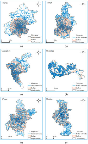
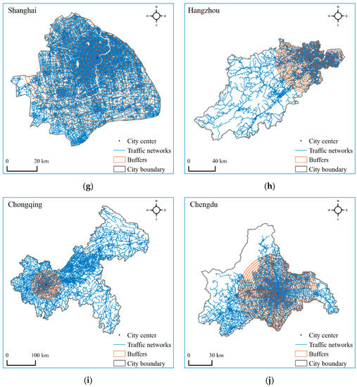
Figure 1.
Traffic networks in 10 Chinese cities based on administrative boundaries in 2016. (a) Beijing; (b) Tianjin; (c) Guangzhou; (d) Shenzhen; (e) Wuhan; (f) Nanjing; (g) Shanghai; (h) Hangzhou; (i) Chongqing; (j) Chengdu. Note: The data extraction for spatial signals is confined by each municipal boundary, so that the spatial information is not complete. In this case, it is improper to estimate the fractal parameter using simple fractal model. It is advisable to apply wave-spectrum scaling analysis to these spatial patterns.
The parameter estimation of any mathematical model needs certain algorithms. The wave-spectral analysis needs two algorithms: one is fast Fourier transform (FFT), and the other is ordinary least squares (OLS) regression method. The former is used to obtain wave spectrums, and the latter is used to estimate spectral exponent. The application of a mathematical methods to concrete problems involves what is called three worlds: real world, mathematical world, and computational world [29,42]. In fact, the computational world can be treated as the bridge between the mathematical world and the real world. Equation (4) describes Fourier transform in pure theoretical form, that is, it is defined in the mathematical world. For the observational data of cities in the real world, the Fourier transform should be replaced by an algorithm termed FFT. Data processing and algorithm application is implemented in the computational world [29]. Applying FFT to the urban density series, we have
where F(k) is the result of FFT, expressed by complex numbers, â is the real part estimated value of the complex number, is the imaginary part estimated value. As indicated above, in theory, = 0 because of the symmetry of correlation function. However, in practice, ≠ 0 owing to random disturbance of spatial signals. Thus, the wave spectrum can be defined as
Based on Equation (16), Equation (6) can be substituted with
where the asterisk “*” denotes an equivalent redefinition of variable F(k) and parameter F0 for simplification. The redefinition does not influence the computational results and analytical process of spatial signals. Taking natural logarithm of both sides of Equation (17) yields a linear equation as below
Thus, by using the OLS method, we can estimate the values of the spectral exponent. In the light of Equation (8), the spectral exponent values can be converted into fractal dimension values and the Hurst exponent. Using these fractal parameters based on spatial signals, we can make spatial analysis for geographical systems.
In summary, the approach of fractal parameter estimation consists of number of steps. The computing process can be implemented step by step as follows. Step 1: Defining study area. In our case studies, a study area is a spatial system of streets and roads within urban envelope. Step 2: extracting spatial datasets. As indicated above, the operation can be carried out by using ArcGIS, a Windows-based collection of Geographic Information Systems (GIS) software. The formula is Equation (13) based on concentric circles. Step 3: generating density series. The formula is Equation (14). The density distribution indicates a spatial correlation function. Step 4: Fourier transform. Applying FFT to density series to yield the wave-spectrum series or the wave-spectrum density series. The formula is Equation (4), which can be discretized by substituting integral for summation. The calculation can be realized through MS Excel. Step 5: wave-spectrum scaling. Fitting Equation (17) or Equation (18) to the datasets of relationships between wave number and wave spectrum series to yield spectral exponents. Step 6: fractal parameter estimation. In the light of Equations (7) and (8) as well as Equations (11) and (12), the spectral exponent values can be converted into fractal dimension and Hurst exponent values (Figure 2). Using these fractal parameters based on spatial signals, we can make spatial analysis for geographical systems.
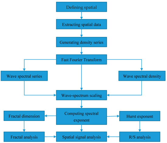
Figure 2.
A flow chart of fractal-based spatial signal analysis for geographical systems. Note: The wave spectral series is based on Equations (4) and (6) as well as Equations (16) and (17), the wave-spectrum density is based on Equations (9) and (10).
3.2. Results and Analysis
The extraction method of spatial signal depends on the research objective. Suppose that we want to investigate urban growth by using traffic networks comprising streets and roads, the system of concentric circles can be employed to measure and calculate the total lengths of routes within certain zones (see File S1). The formula is Equation (13). The length series of streets and roads form the origin spatial signals of urban traffic networks, where trend is concerned, these signals take on unimodal curves (Figure 3 shows two examples). However, we cannot get too more geographical information from these curves. Utilizing Equation (14), we can turn the network length into network density between two adjacent circles. Traffic network density is associated with geospatial diffusion, and spatial diffusion is often based on distance-decay scaling law [19,43]. If the traffic network density follows standard power law, then we can estimate fractal dimension directly. However, due to incomplete patterns of urban network based on administrative boundaries, as well as self-affine growth, the network density decay comes between exponential distribution and logarithmic distribution (Figure 4 shows two examples). In other words, the density distributions of traffic networks do not follow power law in a strict sense, therefore Smeed’s model cannot be used to estimate fractal dimension effectively. It is necessary to make wave-spectral analysis using Equations (15)–(18).
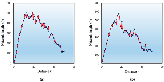
Figure 3.
The spatial signals for traffic network of Beijing and Shanghai cities (2016). (a) Beijing; (b) Shanghai. Note: These spatial signals represent urban traffic lines extracted through concentric circles and Equation (13). Each value reflects a total length of streets and roads falling in two adjacent circles.
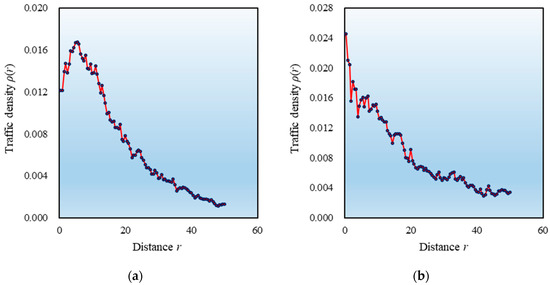
Figure 4.
The patterns of traffic network density distributions of Beijing and Shanghai cities (2016). (a) Beijing; (b) Shanghai. Note: The spatial signals can be turned into density curves of urban traffic networks by using Equation (14). If the density data could be fitted to an inverse power law, we should estimate fractal dimension directly by means of Equation (1). Due to the curves depart from power function, we had to employ the wave-spectrum scaling analysis to estimate fractal dimension.
Based on spatial series of traffic network density, wave-spectrum scaling relations can be examined easily. Using mathematical software Matlab or even MS Excel, we can make Fourier transform for each density series. The wave number can be defined as
where j = 0, 1, 2, …, N−1. According to FFT, the number N must satisfy the following condition
Otherwise, we have to remove a number of numbers at the beginning or at the end of a sequence, or add a set of 0 to the end, so that the length of the sequence becomes the integer power of 2. The circle number of each city is 100. We, either, add 28 zeros to the end of the sequence so that the length of sample path become 128 (N = 27), or remove the last 36 data points, so that the sample path length become 64 (N = 26). The former way (adding 0) is better than the latter way (removing partial data). Compared with deleting 36 data points, adding 28 zeros to the end of the sequence results in less geospatial information loss. After the FFT of density sequence, we can compute wave spectrum by means of Equation (16). Then, by using the least square regression based on Equations (17) and (18), we can make models for wave spectrum scaling relation. For example, for Beijing’s traffic network, the model is
The goodness of fit is about R2 = 0.8543, the spectral exponent is α = 0.9635. Thus the fractal dimension is estimated as Df = 1.9635. For Shanghai’s network density, the model is
The goodness of fit is about R2 = 0.8570, the spectral exponent is α = 0.7707. Consequently, the fractal dimension is estimated as Df = 1.7707. The traffic networks of other cities can be dealt with by analogy (Table 2, Figure 5).
Table 2.
Wave spectrum exponents of urban density and corresponding fractal dimension values (2016).
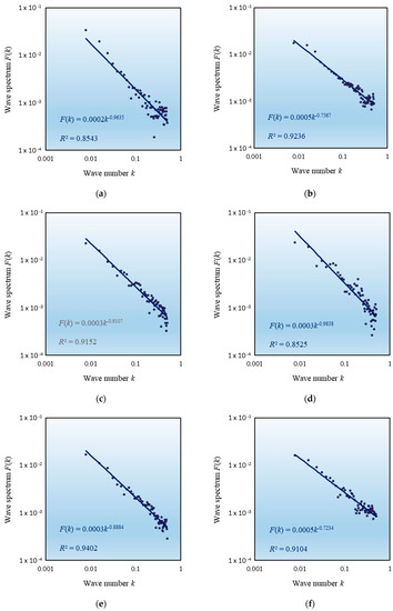
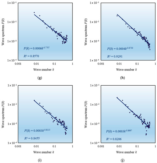
Figure 5.
The wave-spectrum scaling relations between wave numbers and wave spectrums (2016). (a) Beijing; (b) Tianjin; (c) Guangzhou; (d) Shenzhen; (e) Wuhan; (f) Nanjing; (g) Shanghai; (h) Hangzhou; (i) Chongqing; (j) Chengdu. Note: All the spectral exponents were estimated by Equation (17), which is based on Equation (6). By using Equation (8), we can easily turn the spectral exponent values into fractal dimension values.
The fractal dimension estimated by wave-spectrum scaling can be used to replace the radial dimension. The radial dimension has three meanings for spatial analyses: firstly, the degree of space filling: the denser the traffic network of a city, the higher the fractal dimension value; secondly, the degree of spatial homogeneity: the slower the attenuation of traffic network density from a city center to the periphery, the higher the fractal dimension value; thirdly, the degree of spatial correlation: the stronger the accessibility from one place to another, the higher the fractal dimension value. Beijing’s road network has higher degrees of space filling, spatial uniformity, and spatial correlation, its radial dimension is high. Tianjin’s network density is lower than Beijing’s network density, indicating lower spatial filling extent, and its fractal dimension is significantly lower than Beijing’s. Shanghai’s road network has lower spatial homogeneity, that is, the spatial decay rate of the urban network density is higher. Therefore, the radial dimension of Shanghai’s road network is not so high. The distribution of road network in Nanjing is similar, to some extent, to that of Shanghai. In Nanjing, a higher network density attenuation rate leads to relatively low fractal dimension. The traffic network filling degree of Hangzhou is not as high as that of Shanghai, but the network attenuation rate is lower than that of Shanghai. Wuhan is the hub of land and water transportation in Central China. Probably due to the Yangtze River, the road network filling degree of Wuhan is not particularly high. The fractal dimension of the Guangzhou road network is relatively high. The distribution of traffic network in Guangzhou is similar, to a degree, to that of Beijing. Shenzhen’s road network bears lower space filling extent, but has higher spatial homogeneity. In other words, the spatial decay of Shenzhen’s network density is not significant. Therefore, the radial dimension of Shenzhen’s road network is very high. In southwest China, Chengdu is located in the plain area, so its road network bears higher fractal dimension. In contrast, Chongqing is located in the mountainous area, and its road network possesses relatively low fractal dimension. Mountains and rivers reduce the fractal dimension values of urban traffic networks because they affect the space-filling degree of streets and roads in urban regions.
3.3. Cases of Power Spectral Scaling Analysis
In geographical analysis, there are corresponding and conversion relationships between space and time. For comparison and reference, two power spectrum analysis cases of temporal signals can be presented. Complicated signal analysis, based on time series, can be characterized by self-affine record fractal dimension. Despite the similarity in mathematical essence, the form differs from spatial signal analysis. Replacing wave number k and wave spectral density W(k) with frequency f and power spectral density P(f), we can turn Equation (10) into a frequency-spectrum relation as below
in which P0 denotes the proportionality coefficient. Equation (23) can be used to analyze temporal signals through fractal parameters. For example, applying Equation (23) to the time series of urbanization level of China yields a model as follows
The goodness of fit is about R2 = 0.9806, the power spectral exponent is about β = 1.7367 (Figure 6). According to Equation (11), the fractal dimension of self-affine record is about Ds = (5−1.7367)/2 = 1.6316. Thus the Hurst exponent is H = 2−Ds = 0.3684. This suggests an anti-persistence process of urbanization. Urbanization contains a fluctuation process or negative feedback process.
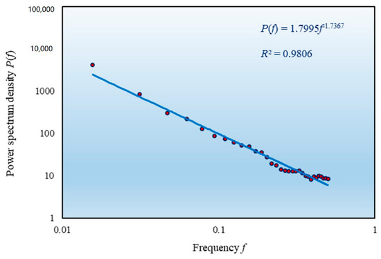
Figure 6.
The power-spectrum scaling relations between frequency and power spectral density (1956–2019). Note: The time series comes between 1949 and 2019. The number of data points is N = 71. According to the requirement of FFT, the data point number must be N = 2j+1, where j = 0, 1, 3, …, int(lnN/ln(2)) ± 1. The best number is N = 64. So, the first 7 data points were removed to meet the needs of the algorithm.
The dynamics of urbanization involves both temporal and spatial processes. In fact, urbanization is associated with urban systems and urban form [44]. The frequency-spectral scaling can be applied to urban form and growth in an urban systems by both temporal and spatial signals. For instance, based on the sample paths of nighttime light (NTL) time series (1992–2013) (see File S2), we can calculate the spectral exponent of urban growth of the cities in Beijing–Tianjin–Hebei region of China (Figure 7, Table 3). The NTL data were originally processed for multi-scaling allometric analyses [45]. The spectral exponents can be converted into self-affine record dimension and self-similar trail dimension, and associated with the Hurst exponent based on R/S analysis [30,46]. The fractal dimension belong to phase space. The results suggest that two types of cities possess higher self-similar fractal dimension values. One is the large cities, such as Beijing and Tianjin, and the other is the cities of self-affine growth such as Zhangjiakou and Qinhuangdao. The Hurst exponent values show that all the growing processes of all these cities bear long memory, moreover, the growing processes of all these cities but Handan bear persistence.
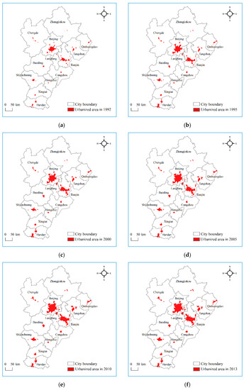
Figure 7.
Urban growth in Beijing–Tianjin–Hebei region reflected by night light data (1992–2013). (a) 1992; (b) 1995; (c) 2000; (d) 2005; (e) 2010; (f) 2013. Note: The changing process of total quantity of nighttime lights (NTL) reflects urban growth. Using time series of night light data, we can make power spectral analysis and estimate the self-affine record dimension for temporal signals. A set of temporal signals reflect spatial signals from cross-sectional angle of view.
Table 3.
The power spectrum exponents, fractal dimension, and Hurst exponent of Chinese cities in Beijing-Tianjin-Hebei region based on time series of night light data (1992–2013).
4. Discussion
The empirical analyses show that the method of wave-spectrum scaling analysis, based on the Fourier transform, can be employed to estimate fractal dimension of spatial signals. Using these fractal parameters, we can make spatial analyses by means of geographical signals. Spatial signal extraction is not limited to traffic networks, but can involve many aspects of geographic systems. Note that fractal approach can only be applied to fractal phenomena. In fact, spatial signals can be divided into two categories and four subcategories (Table 4). If we meet stationary spatial series of geographical signals, the wave-spectrum scaling analysis will be useless. If we meet the trend series of spatial signals with characteristic lengths, generally speaking, the wave-spectrum scaling is useless. Sometimes, the wave-spectrum scaling analysis can be applied to the spatial series satisfying exponential distributions, but the spectral exponent indicates a Euclidean dimension [13,20]. If a self-similar spatial signal series, i.e., the spatial series without characteristic length, is encountered, the method presented in this paper is suitable. If a self-affine spatial signal series appears, the spectral analysis can also be applied to it in a proper way. In particular, if the spatial patterns for signal extraction are not incomplete, the wave-spectrum scaling is indispensable for estimating radial dimension of growing fractal processes. Incomplete spatial patterns result in power law degeneration, and the fractal dimension cannot be directly estimated by Smeed’s model.
Table 4.
Different types of spatial signals and corresponding analytical methods.
Fourier transform and frequency and wave-spectrum scaling is one of important approaches for spatial analysis of geographical fractal phenomena. In urban studies, this method is useful for indirect estimation of fractal dimension, especially when fractal structure is hidden by random noises. Scaling invariance is a universal law in geographical systems. The wave-spectrum scaling analysis has universal applicability. It can be used in different geographical regions to analyze different types of spatial signals. Compared with previous research, this work bears clear novelty. First, the previous works are devoted to theoretical models and fractal parameter relations [19]. In particular, using wave-spectral scaling analysis, new fractal parameter relations are derived [22]. In contrast, this work is devoted to positive analysis of wave-spectral scaling for spatial signals. Second, previous works are mainly devoted to self-affine fractal analysis by empirical approach [20], specifically the relationships between self-affine fractal parameters and self-similar fractal parameters are revealed by means of wave-spectral scaling relations. In contrast, this paper is chiefly devoted to self-similar fractal series. Third, in previous studies, the cases are based on land use patterns of cities [22,29]. In contrast, this paper is devoted to research urban traffic networks.
The shortcomings of this study lies in three respects. Firstly, this paper is actually devoted to 1-dimensional spatial signals. In other words, with the help of statistical average, the 2-dimensional spatial signals are converted into 1-dimensional spatial signals. The 2-dimensional random signals in strict sense cannot be analyzed by means of the wave-spectrum scaling for the time being; Secondly, this paper is principally devoted to self-similar fractal signals, or pseudo self-affine fractal signals, for the self-affine fractal signals, in strict sense, no deep analysis is made in this work. Due to the lack of enough theoretical research on self-affine fractal signals of geographical systems, many principles on self-affine fractal dimension are not yet clear; Thirdly, this paper is mainly devoted to single scaling analysis, while urban systems and traffic networks bear multifractal scaling property. The spatial signals of multiscaling processes can be analyzed by wavelet transform instead of the Fourier transform [47,48]. Wavelet analysis is one of powerful tools for multiscale signal analysis [13,49]. In the future, three respects of research will be carried out. One is to generate the 1-dimensional spatial signal analysis to 2-dimensional spatial signal analysis, the other is to make theoretical and positive studies on self-affine fractal signals in complex systems, and the third is to make wavelet analysis on geographical signals based on multiscaling spatial processes.
5. Conclusions
The Fourier transform and wave-spectrum scaling relation can be applied to fractal-based spatial signal analyses. The academic contribution of this article to science includes two aspects. One is to propose an analytical framework based on wave-spectrum scaling for geographical spatial signals, and the other is to demonstrate that traffic network density distribution follow wave-spectrum scaling law. The first contribution is the writing goal of this paper, and the second contribution is the by-product of this study. The complete analytical processes and cases are presented. Where wave-spectrum scaling analysis method is concerned, the main points of this work are as follows: Firstly, if the self-similar fractal structure of spatial signals is concealed by random noises, or spatial patterns are not incomplete for signal extraction, the wave-spectrum scaling relation can be utilized to estimate fractal dimension. By changing spatial signals to density distribution, we can model the distribution with scale-free correlation function, then the correlation function can be converted into wave-spectrum density by the Fourier transform. Further, using the power law relation between wave number and wave spectrum, we can calculate spectral scaling exponent. The spectral exponent can be turned into the fractal dimension, which can be employed to make spatial analyses for geographical signals. Secondly, if spatial signals bear self-affine fractal property, we can use wave-spectrum scaling to compute the self-affine record dimension. Then, the anisotropic fractal process can be treated as isotropic fractal process approximately. Thus, the fractal dimension of self-affine records can be converted to the fractal dimension of self-similar trails. Combining the self-affine fractal parameter and the self-similar fractal parameter, we can make spatial analysis for geographical signals. Thirdly, the wave-spectrum scaling can be naturally applied to temporal signals of geographical systems. If we have a time series representing temporal signals of geographical systems, e.g., the level of urbanization, we can apply the wave-spectrum scaling to the dataset. If the temporal signal bears fractal property, we will be able to work out the self-affine record dimension. By means of the fractal dimension of self-affine record, we can make time series analysis for the temporal signal of urban evolution.
Supplementary Materials
The following are available online at https://www.mdpi.com/2076-3417/11/1/87/s1. File S1: Datasets of 10 Chinese urban traffic networks for fractal-based wave spectral analysis (Excel). File S2: Datasets of nighttime lights of cities in Beijing–Tianjin–Hebei region of China (1992–2013).
Author Contributions
Conceptualization, Y.C. and Y.L.; methodology, Y.C.; software, Y.L.; validation, Y.C.; formal analysis, Y.C.; investigation, Y.C.; resources, Y.L.; data curation, Y.L.; writing—original draft preparation, Y.C.; writing—review and editing, Y.C.; visualization, Y.L.; supervision, Y.C.; project administration, Y.C.; funding acquisition, Y.C. All authors have read and agreed to the published version of the manuscript.
Funding
This research was funded by the National Natural Science Foundations of China, grant numbers 41590843 & 41671167.
Acknowledgments
The nighttime light dataset (1992–2014) come from American NOAA National Centers for Environmental Information (NCEI). We would like to thank the two anonymous reviewers whose constructive comments were helpful in improving the quality of this paper.
Conflicts of Interest
The authors declare no conflict of interest. The funders had no role in the design of the study; in the collection, analyses, or interpretation of data; in the writing of the manuscript, or in the decision to publish the results.
References
- Shannon, C.E. A mathematical theory of communication. Bell Syst. Tech. J. 1948, 27, 379–423. [Google Scholar] [CrossRef]
- Guariglia, E. Entropy and fractal antennas. Entropy 2016, 18, 84. [Google Scholar] [CrossRef]
- Cramer, F. Chaos and Order: The Complex Structure of Living Systems; VCH Publishers: New York, NY, USA, 1993. [Google Scholar]
- Pincus, S.M. Approximate entropy as a measure of system complexity. PNAS 1991, 88, 2297–2301. [Google Scholar] [CrossRef] [PubMed]
- Ryabko, B.Y. Noise-free coding of combinatorial sources, Hausdorff dimension and Kolmogorov complexity. Probl. Peredachi Inf. 1986, 22, 16–26. [Google Scholar]
- Chen, Y.-G.; Wang, J.-J.; Feng, J. Understanding the fractal dimensions of urban forms through spatial entropy. Entropy 2017, 19, 600. [Google Scholar] [CrossRef]
- Guariglia, E. Primality, fractality, and image analysis. Entropy 2019, 21, 304. [Google Scholar] [CrossRef] [PubMed]
- Sparavigna, A.C. Entropies and Fractal Dimensions. Philica. 2016. Available online: https://hal.archives-ouvertes.fr/hal-01377975 (accessed on 23 November 2020).
- Zmeskal, O.; Dzik, P.; Vesely, M. Entropy of fractal systems. Comput. Math. Appl. 2013, 66, 135–146. [Google Scholar] [CrossRef]
- Chen, Y.-G. Equivalence relation between normalized spatial entropy and fractal dimension. Phys. A 2020, 553, 124627. [Google Scholar] [CrossRef]
- Chowdhury, P.N.; Shivakumara, P.; Jalab, H.A.; Ibrahim, R.W.; Pal, U.; Lu, T. A new fractal series expansion based enhancement model for license plate recognition. Signal Process. Image Commun. 2020, 89, 115958. [Google Scholar] [CrossRef]
- Feder, J. Fractals; Plenum Press: New York, NY, USA, 1988. [Google Scholar]
- Liu, S.-D.; Liu, S.K. An Introduction to Fractals and Fractal Dimension; Meteorological Press: Beijing, China, 1993. [Google Scholar]
- Takayasu, H. Fractals in the Physical Sciences; Manchester University Press: Manchester, UK, 1990. [Google Scholar]
- Brockwell, P.J.; Davis, R.A. Time Series: Theory and Methods, 2nd ed.; Springer: Berlin/Heidelberg, Germany, 1998. [Google Scholar]
- Clark, C. Urban population densities. J. R. Stat. Soc. 1951, 114, 490–496. [Google Scholar] [CrossRef]
- Berry, M.V.; Lewis, Z.V. On the Weierstrass-Mandelbrot fractal function. Proc. R. Soc. Lond. Ser. A 1980, 370, 459–484. [Google Scholar]
- Smeed, R.J. Road development in urban area. J. Inst. High. Eng. 1963, 10, 5–30. [Google Scholar]
- Chen, Y.-G. Exploring the fractal parameters of urban growth and form with wave-spectrum analysis. Discret. Dyn. Nat. Soc. 2010, 2010, 974917. [Google Scholar] [CrossRef]
- Chen, Y.-G. A wave-spectrum analysis of urban population density: Entropy, fractal, and spatial localization. Discret. Dyn. Nat. Soc. 2008, 2008, 728420. [Google Scholar] [CrossRef]
- Batty, M.; Longley, P.A. Fractal Cities: A Geometry of Form and Function; Academic Press: London, UK, 1994. [Google Scholar]
- Chen, Y.-G. Fractal analytical approach of urban form based on spatial correlation function. Chaos Solitons Fractals 2013, 49, 47–60. [Google Scholar] [CrossRef]
- Chen, Y.G.; Wang, Y.H.; Li, X.J. Fractal dimensions derived from spatial allometric scaling of urban form. Chaos Solitons Fractals 2019, 126, 122–134. [Google Scholar] [CrossRef]
- Frankhauser, P. The fractal approach: A new tool for the spatial analysis of urban agglomerations. Popul. Engl. Sel. 1998, 10, 205–240. [Google Scholar]
- Frankhauser, P.; Sadler, R. Fractal analysis of agglomerations. In Natural Structures: Principles, Strategies, and Models in Architecture and Nature; Hilliges, M., Ed.; University of Stuttgart: Stuttgart, Germany, 1991; pp. 57–65. [Google Scholar]
- White, R.; Engelen, G. Cellular automata and fractal urban form: A cellular modeling approach to the evolution of urban land-use patterns. Environ. Plan. A 1993, 25, 1175–1199. [Google Scholar] [CrossRef]
- Hyde, M.W., IV. Controlling the spatial coherence of an optical source using a spatial filter. Appl. Sci. 2018, 8, 1465. [Google Scholar] [CrossRef]
- Chen, L.; Zheng, L.-J.; Yang, J.; Xia, D.; Liu, W.-N. Short-term traffic flow prediction: From the perspective of traffic flow decomposition. Neurocomputing 2020, 413, 444–456. [Google Scholar] [CrossRef]
- Chen, Y.-G. Fractal dimension analysis of urban morphology based on spatial correlation functions. In Mathematics of Urban Morphology; D’Acci, L., Ed.; Springer Nature: Birkhäuser, Switzerland, 2019; pp. 21–53. [Google Scholar]
- Mandelbrot, B.B. The Fractal Geometry of Nature; W. H. Freeman and Company: New York, NY, USA, 1982. [Google Scholar]
- Harvey, D. Explanation in Geography; Edward Arnold Ltd.: London, UK, 1969. [Google Scholar]
- Chen, Y.-G. Mathematical Methods for Geography; Science Press: Beijing, China, 2011. [Google Scholar]
- Chen, Y.-G. The spatial meaning of Pareto’s scaling exponent of city-size distributions. Fractals 2014, 22, 1450001. [Google Scholar] [CrossRef]
- Dai, M.-F.; Zhang, C.; Li, L.; Wu, W. Multifractal and singularity analysis of weighted road networks. Int. J. Mod. Phys. B 2014, 28, 1450215. [Google Scholar] [CrossRef]
- Prada, D.; Montoya, S.; Sanabria, M.; Torres, F.; Serrano, D.; Acevedo, A. Fractal analysis of the influence of the distribution of road networks on the traffic. J. Phys. Conf. Ser. 2019, 1329, 012003. [Google Scholar] [CrossRef]
- Rodin, V.; Rodina, E. The fractal dimension of Tokyo’s streets. Fractals 2000, 8, 413–418. [Google Scholar] [CrossRef]
- Sahitya, K.S.; Prasad, C.S.R.K. Modelling structural interdependent parameters of an urban road network using GIS. Spat. Inf. Res. 2020, 28, 327–334. [Google Scholar] [CrossRef]
- Valério, D.; Lopes, A.M.; Machado, J.A.T. Entropy analysis of a railway network complexity. Entropy 2016, 18, 388. [Google Scholar] [CrossRef]
- Wang, H.; Luo, S.; Luo, T. Fractal characteristics of urban surface transit and road networks: Case study of Strasbourg, France. Adv. Mech. Eng. 2017, 9, 1687814017692289. [Google Scholar] [CrossRef]
- Long, Y.-Q.; Chen, Y.-G. Fractal characterization of structural evolution of Beijing, Tianjin and Hebei transportation network. Hum. Geogr. 2019, 34, 115–125. [Google Scholar]
- Guariglia, E. Harmonic Sierpinski gasket and applications. Entropy 2018, 20, 714. [Google Scholar] [CrossRef]
- Casti, J.L. Would-Be Worlds: How Simulation Is Changing the Frontiers of Science; John Wiley and Sons: New York, NY, USA, 1996. [Google Scholar]
- Lengyel, B.; Bokányi, E.; Di Clemente, R.; Kertész, J.; González, M.C. The role of geography in the complex diffusion of innovations. Sci. Rep. 2020, 10, 15065. [Google Scholar] [CrossRef]
- Knox, P.L.; Marston, S.A. Places and Regions in Global Context: Human Geography, 5th ed.; Prentice Hall: Upper Saddle River, NJ, USA, 2009. [Google Scholar]
- Long, Y.-Q.; Chen, Y.-G. Multi-scaling allometric analysis of the Beijing-Tianjin-Hebei urban system based on nighttime light data. Prog. Geogr. 2019, 38, 88–100. [Google Scholar]
- Hurst, H.E.; Black, R.P.; Simaika, Y.M. Long-Term Storage: An Experimental Study; Constable: London, UK, 1965. [Google Scholar]
- Yang, L.; Su, H.-L.; Zhong, C.; Meng, Z.-Q.; Luo, H.-W.; Li, X.-C.; Tang, Y.-Y.; Lu, Y. Hyperspectral image classification using wavelet transform-based smooth ordering. Int. J. Wavelets Multiresolution Inf. Process. 2019, 17, 1950050. [Google Scholar] [CrossRef]
- Zheng, X.-W.; Tang, Y.-Y.; Zhou, J.-T. A framework of adaptive multiscale wavelet decomposition for signals on undirected graphs. IEEE Trans. Signal. Process. 2019, 67, 1696–1711. [Google Scholar] [CrossRef]
- Du, W.T.; Zeng, Q.; Shao, Y.-M.; Wang, L.-M.; Ding, X.-X. Multi-scale demodulation for fault diagnosis based on a weighted-EMD de-noising technique and time–frequency envelope analysis. Appl. Sci. 2020, 10, 7796. [Google Scholar] [CrossRef]


Publisher’s Note: MDPI stays neutral with regard to jurisdictional claims in published maps and institutional affiliations. |
© 2020 by the authors. Licensee MDPI, Basel, Switzerland. This article is an open access article distributed under the terms and conditions of the Creative Commons Attribution (CC BY) license (http://creativecommons.org/licenses/by/4.0/).