Abstract
The video game industry has evolved significantly, with different genres becoming popular over time, but how to visualize such information by curating data into a form that makes it easier to identify and understand the trends is quite an interesting research topic. This research focuses on producing an animation of aesthetically pleasing two-dimensional (2D) undirected graphs based on PC video game datasets. The data are further analyzed for developing a web-based application giving users the ability to control and create the animation of a graph. To make it easier to understand the animation of a graph, the changes between the displays of the previous and the following periods are set as small as possible, allowing a user to grasp the differences of the graph’s structure faster. A genetic algorithm-based undirected graph drawing that minimizes both the aesthetic criteria and mental map cost are proposed in this research to tackle this problem. Furthermore, based on our experiments, we could find the best period to start with, so we do not necessarily need to start from the first period to calculate the animation result. Our experiment results proved that a smoother animation could be achieved, and information is better preserved throughout the animation.
1. Introduction
Graphs are prevalent data structures produced with computers and represent and visualize data from various research fields. Drawing graphs or network diagrams is an illustration of their vertices and edges. Vertices are used to symbolize an item or entity, while edges represent the relationship among those items or entities.
Visualizing graph data is important, because good visualizations can represent patterns and insights and support or falsify hypotheses. Much effort has been directed toward making such visually pleasing diagrams. In 1989, Kamada and Kawai [1] presented an algorithm to solve this problem. They drew general graphs based on a spring model and suggested that the total balanced layout is at least as important as the reduction of edge crossings for human understanding. In their model, the total balance condition is formulated as the square summation of the differences between desirable distances and real ones for all the pairs of vertices.
Another algorithm of force-directed graph drawing was also presented by Fruchterman and Reingold [2]. They were inspired by a natural system such as springs and macro-cosmic gravity, where the vertices behave as atomic particles or celestial bodies, exerting attractive and repulsive forces on one another; the forces induce movement.
In 1996, Davidson and Harel (DH) [3] proposed a drawing algorithm using simulated annealing to reduce the energy of a system. The problem of drawing a graph is restated as a problem in minimizing the energy and can be considered one of the optimization problems. Many aesthetic criteria [4] can be regarded, and the generally accepted ones include:
- Uniform spatial distribution of the vertices.
- Minimum total edge length on the precondition so that the distance between any two vertices is not less than a given minimum value.
- Uniform edge length.
- Small angle between edges incident on the same vertex.
- Similar angles between edges incident on the same vertex.
- Minimum number of edge crossings.
- To exhibit any existing symmetric features.
These criteria can be combined to form a multi-criterion weighted sum objective function that measures the quality of a graph, which is then optimized by search-based methods (optimization methods). By applying a metaheuristic algorithm such as simulated annealing, a user can choose a flexible energy function by utilizing its weights to emphasize which aesthetic standard would be prioritized. Following these directions, many drawing algorithms have emerged using different metaheuristic algorithms, such as Stochastic Hill Climbing (HC) [5], Genetic Algorithm (GA) [4,6,7,8], Particle Swarm Optimization (PSO) [9] and Tabu Search (TS) [10], and all of them have shown promising results.
A graph can be drawn in many forms, where the position of each vertex could be restricted to a layer, circle or a grid point, while the edges can also be drawn not only as a straight line but, also, polygonal lines or curves. The main problem is arranging the vertices and edges; thus, it could affect the aesthetics of a graph and its comprehension and application. The problem gets worse if the graph changes over time by adding and deleting nodes and edges (dynamic graph drawing), and the goal is thus also to preserve a user’s mental map regarding a changing graph.
In 1991, Eades et al. [11] proposed the mental map concept in graph drawing, in which predictability and traceability are identified so that movement is easy to follow. Preserving a user’s mental map is important in dynamic graph drawing in order to quickly recognize and understand the redrawn layout of a modified graph. Figure 1 shows a simple example of how important mental map preservation is in a dynamic graph drawing.
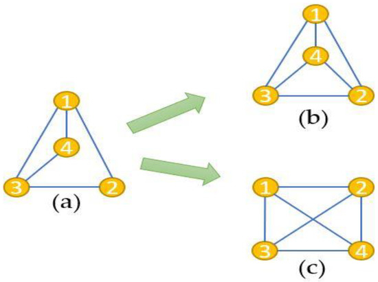
Figure 1.
The importance of mental map preservation ((a)—main shape, (b)—adding edge with mental map preservation, (c)—adding edge without mental map preservation).
Our current research focuses on drawing undirected graphs where each vertex is not restricted, and each edge is a straight line. To draw graphs nicely, and considering dynamic stability, we used a genetic algorithm (GA) with the fitness value based on the aforementioned requirements. This allows our system to adjust the relative weight accordingly, preserve a better mental map or get a better appearance. By creating a smooth animation of a precalculated undirected graph by preserving a user’s mental map, we developed a web-based application that can produce and show the smooth animation of multiple undirected graphs of video game data.
We made the following contributions. First, we proposed a mental map preserving algorithm for an undirected graph using the GA. Second, we developed a web-based application that allows users to create and control the animation of graphs. Third, our proposed system can be generalized and applied in various domains, such as archiving data from the work of Paszkiel et al. [12] or movie datasets or can be used to visualize word embedding or topic modeling.
The rest of the paper is organized as follows. In Section 2, we will explain the proposed system, including the system architecture design and methods used in this system. In Section 3, we will demonstrate the results of the experiment that we conducted. In the last two sections, we will discuss, conclude our research and point out some possibilities for future works.
2. Materials and Methods
2.1. System Overview
Our algorithm can be applied to every dataset, as long as the relationship between two entities can be calculated, and we used a video game dataset as our main dataset. Our graph is a pictorial representation of the vertices and edges of a graph, shown in Figure 2, where a vertex represents an item or entity, while an edge is used to represent the relationship or similarity between two objects. The main problem is how to arrange these vertices and edges that could affect the understandability, usability and aesthetics of a graph.
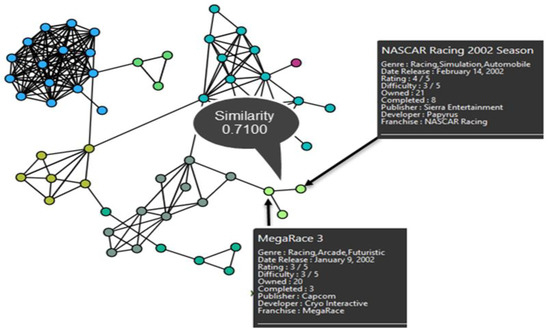
Figure 2.
Example of our graph.
2.2. System Architecture
The system architecture is shown in Figure 3. It is based on basic web application architecture, where it consists of the front end and back end. The front-end part handles a user’s input command and displays the result that was given by our web server.
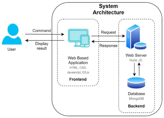
Figure 3.
System architecture.
Through the web application, a user can filter the data he/she wants to be drawn and fully control the animation, including play, pause and choice of the next or previous periods to be shown. Most of the calculation of the node positions is done on the server side, which will then be stored in our database. Figure 4 shows our front-end interface where a user can filter data, such as the number of displayed nodes; the threshold for similarity link and algorithm simplicity; the year of release; user ratings; difficulty ratings; number of people owning the game; number of people who completed the game, a text-based filter for the title, genre, publisher and developer of the game and, also, the set period window size and its step size on the animation set before performing the animation calculation. Smaller period window sizes mean lesser nodes in each period, while a smaller step size gives minor visual changes during the animation.
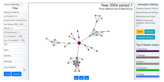
Figure 4.
Front-end interface.
The web server will receive an input filter as a request from the front end and retrieve the necessary data from the database during the calculations. The retrieved data will then be calculated using our algorithm to produce the best position for each node period by period and then stored in the database. Using GA, where it is slow to converge and needs much memory space, our experimental results concluded that a higher number of nodes (above 100) takes too much processing time, and the drawing of too many nodes could cause a user to be unable to comprehend any information. Therefore, we implemented a simplification algorithm to reduce the processing time and make the information easier to understand.
Our simplification algorithm works by combining several similar nodes (nodes of the same genre) into one larger node by checking it against a threshold. This threshold is based on a simplification threshold filter that can be adjusted in the filter area. The default threshold setting is auto, where aggregating nodes reduce the number of nodes for every group, starting from the largest group size until the total number of nodes is below 100. As a result, if a user wants to see more details during animation, he/she can pause the animation and click on a merged node to expand into several nodes based on its original filter. D3′s force-directed algorithm handles the movement of the expanded nodes. Table 1 shows the details of the hardware and software environments of our experiments.

Table 1.
System environment.
Once the calculation process is done and stored in the database, a user can play the animation. For every period, the front-end part requests the server for the data in that period and displays it accordingly, so each node moves to its previously calculated positions.
2.3. Dataset and Similarity Calculation
The dataset used for this research was collected from GameFAQs.com on 24 April 2019. It consists of 63,952 games with English titles from 1985 to 2019. We performed some preprocessing by removing the games that were not rated at all and were left with 36,696 games. Next, we defined the relationship between each data (node) using similarity calculations. Defining similarity is one of the important key points in graph drawing, as different similarities will provide different results for an undirected graph. The higher the value, the more similar the two nodes are. Equation (1) shows how we define our similarity function.
S (Oi, Oj) = ω1 f (A1i, A1j) + ω2 f (A2i, A2j) +...+ ωn f (Ani, Anj)
The similarity function is based on a simple linear equation with a manually determined weight for each attribute. S is our similarity value, and Oi and Oj are our pair of nodes. ωk is our weight for attribute k, and f (Aki and Akj) is a function to determine the difference between attribute k of nodes i and nodes j, and it returns a value between 0 and 1, where 0 means no similarity and 1 means the most similarity.
For the numerical value features (rating and difficulty), we first calculated the difference of their values and then normalized them with the max value, which was five. Table 2 shows how we defined our similarity weights for each attribute. We decided to give the highest weight to the “Genre” attribute, as we perceived it to be the most effective attribute in the similarities between games.
Table 2.
Similarity weight assignment.
2.4. Transition Animation
A bad transition technique of visualizing evolving graphs can cause distraction to the user’s mental map. When the movements of graph layout iterations are mixed with the additions and removals of nodes and edges simultaneously, the user may not be able to perceive the changes appropriately. We applied Walter’s work on visualizing evolving graphs [13], because without that, the changes will be difficult to recognize.
Figure 5 is an example to show our transition animation procedure from the first period to the next period. To avoid changing the layout simultaneously, Walter introduced a way of displaying the layout iteratively, which was modified to fit our system. Firstly, we removed all nodes and edges slowly; we then moved each node to its position and, finally, showed the rest of the nodes and edges. The user can see the removal and insertion changes much better than changing them simultaneously, thus preserving the user’s mental map.
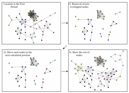
Figure 5.
Transition animation procedure.
2.5. Genetic Algorithm
2.5.1. Fitness Function
The input of our GA algorithm is a graph G = (V, E), where V is the set of nodes, and E is the set of edges. Each candidate solution is encoded as a vector containing coordinates (, ) and its previous position (’, ’), if it existed, to calculate the mental map preservation. We use several aesthetic criteria that will be minimized, and they are composed by a weighted sum. A user will define these weights to adjust the graph drawing.
Equation (2) is our fitness function f, where is our weight for each term, is the distance between node i and node j using the Euclidean distance, is the distance between node i and center c using the Euclidean distance and size is the number of nodes inside a merged node. Every term will be normalized by dividing it by its first calculated value; hence, a lower value will be below one.
By maximizing the distance among nodes, they can spread evenly. We added into consideration, so the larger a node size, the greater the distance between the node and the other nodes; then, a bigger size node can have enough space when a user wants to expand it to see more detail.
The next term is the uniform edge length, where all edges supposedly have a uniform length to achieve a better aesthetic result. A similarity value is also used between them so that the more similar two nodes are, the shorter the length is. We defined to be the shortest paths between node i and j based on its similarity value. Our third term is basically used to pull every node to the center of a screen instead of letting them stay along the screen’s boundary. The last criteria used is the greadability.js to measure our graph readability, where the input is our graph (V and E), and the output includes four global graph readability metrics [14]. All of these metrics are between [0, 1], and higher numbers indicate better layouts, so the average of all the metrics is our third term in the fitness function. We consider these three terms sufficient to draw a good layout, as they cover most of the aesthetic criteria.
2.5.2. Genetic Operator
The genetic operator in this paper consists of three methods: Crossover, Mutation and Inversion. Our Inversion and Mutation operators are based on the previous work of Zhang et al. [4] on a genetic algorithm graph drawing, as it was proven to help draw large cycles with no chords as convex polygons and can reach an optimum solution faster.
Choosing a desirable crossover operator in graph drawing is hard. Here, a desirable crossover should generate an offspring that is similar to its parent. Our crossover operator, called single-link crossover, will exchange a chain of connected points, thus inheriting characteristics much better than only exchanging a single point. As shown in Figure 6, both offsprings obtained a much better fitness value as they reduced the edge-crossing while still maintaining some characteristics from their parents.
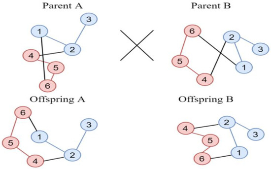
Figure 6.
Single-link crossover.
We have two types of mutation operators that will be sequentially applied. The first one, called a nonuniform mutation [4], is defined in Equation (3), where S = (,, …, , …, ) is a chromosome (a node is (, ), in this case), and element is selected to be mutated:
In Equation (3), is a random value between 0 or 1, is our current generation, [, ] is the lower and upper bounds for and function returns a value in the
range such that the probability of returning 0 increases when value increases. The equation for this function is shown with more detail in Equation (4):
where is our max number of generations, and is our learning parameter chosen by a user. This property of nonuniformity will search a broad area in the initial generation while moving on to the local one in later stages. It tunes the solutions in later stages of evolution.
The second one is called the single-vertex neighborhood mutation [4], which chooses a random node and moves it to a random point on a circle of decreasing radii, along with the generation. Suppose vertex is chosen; then, is the new coordinate of , defined in Equation (5):
where , and is a random number between . is the ideal edge length calculated based on the number of nodes, and our drawing size is shown in Equation (6):
where is the maximum length of a side of a square area display, and diameter is the diameter of the visible graph. In other words, the diameter is the distance between the farthest pair of nodes, and we set the value to be , where is the total number of nodes. This method also has the nonuniformity to make a broad search in the early stages and a more focused search on the later stages.
We also implemented a relinking path algorithm at each generation with a certain percentage. Path relinking is a search intensification strategy [15]. With this research, we want to verify if a path relinking could work with GA to get a better drawing result, just like Dib and Rodgers [10], on a graph drawing by combining Tabu search with path relinking. Figure 7 shows how our relinking path process works. The path relinking algorithm starts with two solutions, a source and a target solution, where the target solution usually has a better fitness value than the source solution. Based on Dib and Rodgers [10], here, the most distant solution is the one with the maximum summed distance of each node to the node of the best solution. We then start moving each node in source A towards each node position in target B, shown in Figure 7, with the movement size of a random value between 0 and PRstepsize, which is defined by the user. This PRstepsize starts with a large value and decreases at each iteration, so that, at later iterations, a minor movement is made to achieve better precision. At every iteration, after moving every node, we calculated its fitness value and stored the best solution. The best solution found during the moving process of source A to target B will be replaced by the worst solution in the current generation if it has a better value.
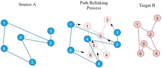
Figure 7.
Path relinking example.
2.6. Mental Map Preservation
This subsection describes how we tackle the preservation of a mental map by combining both the aesthetic criteria and mental map preservation criteria to be one energy function to be minimized. We define our mental map cost between the previous drawing and current drawing , defined in Equation (7). Note that means both drawings are the same; hence, a larger value means a higher degree of difference between two drawings. The position of an overlapped node is based on the previous drawing, so that the preservation is easier to do.
Our mental map cost is based on what Bridgeman and Tamassia [16] proposed, which is shown in Equations (8)–(10). Although there are many similarity measurements, we only use ranking, nearest neighbor within and nearest neighbor between. Using only these three measurements is good enough to preserve a mental map while not necessarily fixing the overlap node positions between two periods. As our main purpose is to create a smooth transition between two graphs—that is, between our previous graph and our current graph —we only measured based on the node that exists in both periods.
We used a similar method as our fitness function, where was our weight for each term. The first term is called ranking [16], used to measure the relative horizontal and vertical positions of a point. Equation (8) shows our ranking measurement:
where the upper bound is to normalize the value to be between 0 and 1; also noted here is that the upper bound is taken as instead of , where the actual maximum value occurs when a point moves from one corner of the drawing to the opposite corner. The motivation for this is simply that it scales the measurements more satisfactorily. Right and above are the numbers of nodes to the right and above of v (similarly, the ). This measures how many changes have happened on a node’s viewpoint between the previous drawing and the current drawing.
where is the upper bound for the normalization of the number of nodes that exist in both layouts, while is the nearest neighbor of node . Our second term, called nearest neighbor within [16], shown in Equation (9), is the idea that a node neighborhood in the previous layout should be its neighborhood as well in the current layout. This term calculates the number of nodes that have their nearest neighbor changed.
Our last term, called the nearest neighbor between [16], shown in Equation (10), is similar to the nearest neighbor within, except this term idea is that a node nearest neighbor in the current layout should be itself from the previous layout. This will make a node bound within its previous position but free to move as long as its nearest neighbor is itself. We used the unweighted version for both nearest-neighbor terms, where we did not count the number of nodes between and .
Multiple terms were not included in our mental map cost function. We also removed other terms that Lee et al. [14] used in their SA to make the computations faster, as, in general, GA needs much more resources than SA.
In the work of Lee et al. [14], for solving a problem of combining two cost functions with different scales, they considered the energy cost and mental map cost independently in their SA algorithm. Our research faced a similar problem, so instead of considering them independently, we gradually considered the mental map cost across generations.
We started with weight of the mental map cost on the initial generation and started considering a half-weight of the mental map cost when reaching of the generation and, finally, the full weight of the mental map cost after of the generation. In this way, our system prioritizes creating an excellent aesthetic drawing during the early generations and then considers the mental map cost during later generations.
3. Results
3.1. Experiments Parameter
This subsection shows our experimental parameters for evaluating the performance of our algorithm on minimizing both the aesthetic cost and mental map cost. All of our experimental parameter values are shown in Table 3. We experimented with multiple population sizes in the range of 1–100, and we concluded that a population size of 10 gives a much better performance in time and reaches roughly the same results compared with population sizes larger than 10.
Table 3.
GA parameter values of the experiment.
The generation count parameter needed to be tuned according to the total nodes drawn, where more generation gives better results on a larger number of nodes and edges. Additionally, we used a higher probability of the mutation operation, because we observed that a crossover operation is not good enough to transfer information from parents to their children.
Table 4 shows our fitness weight settings. Our first four fitness types are our aesthetic criteria, while the last three are our mental map preservation criteria. We concluded that giving the highest attention to the uniform edge length in aesthetic criteria gives the best results, because we have to prioritize the nodes that have the relationship to be drawn near each other. Additionally, note that we provided the lowest weight value to the distance to the center, because too much weight could cause all nodes to move toward the center while ignoring other fitness concerns. We gave a value of 1 for our mental map preservation, which was higher than the aesthetic criteria weight, so we could prioritize the preservation cost more than the aesthetic criteria.
Table 4.
Fitness weight settings.
3.2. Experimental Results
We started our experiment by using several methods to consider the weight of the mental maps. The first method was to consider the mental map weight at the initial generation. The second method was to consider the mental map weight when the current generation reached a certain point. The last method was to consider changing the mental map weight gradually across generations. In our experiment, we used the set of video game data from the year 2000. We defined our window size as 60 days or two months, with a moving step size of 30 days or a month. The first period was from January to March, while the second period was from February to April, and so on. We could get overlapped nodes in the second period, which means the games that were released between February to March and were used for getting the relations between nodes to preserve the mental map. We calculated them based on the total of 73 nodes with 34 overlapped nodes of games from the second period of the year 2000.
The results in Figure 8 are from several methods with different timings to start considering the mental map cost and are shown as the fitness values of the best solution in each generation. We can conclude that considering the mental map weight since the start of the generations gives the best preservation, as during the initial generation, every node was placed where they previously calculated. Additionally, there was not much aesthetic cost differences between all the methods, which indicates that our GA is better at preserving the mental maps by holding the nodes in their previous positions rather than generating a good aesthetic layout and then moving the nodes to their previous positions.
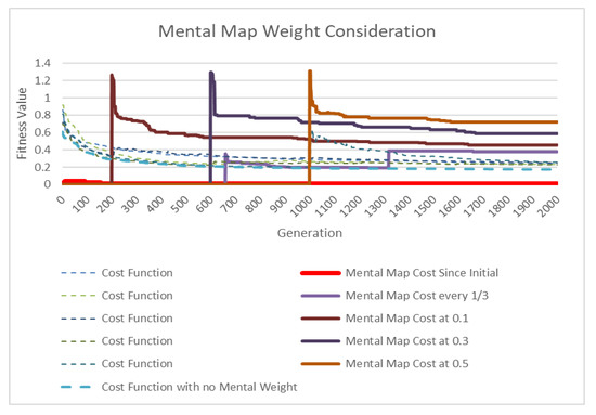
Figure 8.
Mental map weight consideration difference.
Our following experimental results were about implementing the Path Relinking (PR) algorithm in our system. We experimented on several dataset periods, including 2000, 2004 and 2013, and we only considered the first period for these years. The results are shown in Table 5, where is the size of the nodes, and is the total edges of that dataset.
Table 5.
Experiment results of various PR implementations.
Through Table 5, we can see that adding PR to our system indeed helps in finding a better fitness value, even if it is not that significant compared with the case without using PR, as shown in all our experiment results. We concluded that adding PR (both forward and backward) incurred some costs, as it roughly doubled our processing time in each dataset, as shown in Table 5. This proves that PR indeed works well with Tabu Search, but not with GA, where every worse solution found during Tabu Search can prevent PR from recalculating them, thus making the process faster. In our system, we did not record these worse solutions, and so, PR kept on calculating the exact solutions all over again. We did add a random movement so that the same solutions were unlikely to occur.
Figure 9 shows the best fitness value in each generation for datasets 2004 and 2013, respectively. In every experiment, those using PR always converged much earlier than those without PR, as we can see from the curves on both graphs. However, once they reached convergence, using PR gave no better results than the ones without PR, and all of the experiments reached roughly the same results. We concluded that using PR gives a considerably faster convergence rate but not better results from these experiments.
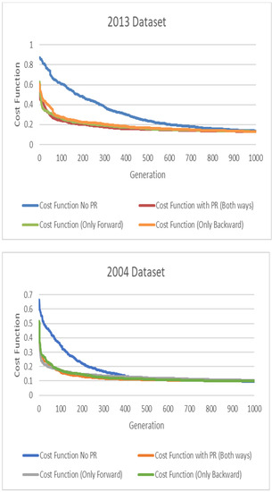
Figure 9.
Experimental results of the PR implementation per generation.
3.3. Mental Map Evaluation
We used the same experiment parameter as our mental weight consideration and the dataset, which included the games of the first to the third period of the year 2000. Figure 10 shows how the user’s mental map is destroyed if no algorithm is applied to preserve the mental map. We can see not only the changes in position, but, also, most of the shapes made by the nodes could destroy the user’s previous knowledge about each node group position, especially shape. Figure 11 shows how our algorithm preserves the mental map, so that the previous information is not completely lost.
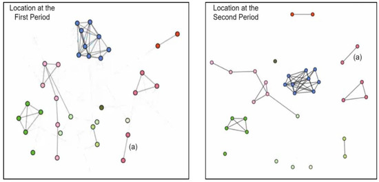
Figure 10.
Transition from the first to the second period without any mental map preservation.
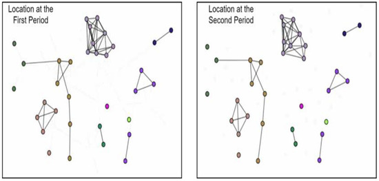
Figure 11.
Transition from the first to the second period with mental map preservation.
Next, our mental map evaluation involved the Generalized Procrustes Analysis (GPA) [17]. The general idea of the Procrustes analysis is to analyze the statistical shape variations [18]—that is, to find a degree of similarity between different shapes in a set. This fits the case of our undirected graph, as each node’s position does not have any reference shapes.
We used the Python SciPy Procrustes Analysis [19] library to test the similarities of the two graphs. Our first input was the coordinates of overlapped nodes in the previous layout, which were compared with the second input coordinates of the overlapped nodes in the new layout. Figure 12 shows our Procrustes analysis results, based on the same datasets as previously used (the year 2000 and periods 2 and 3). In this figure, means considering the mental map preservation, and we can see the differences of the Procrustes scores between those that consider the mental map cost and those that do not.
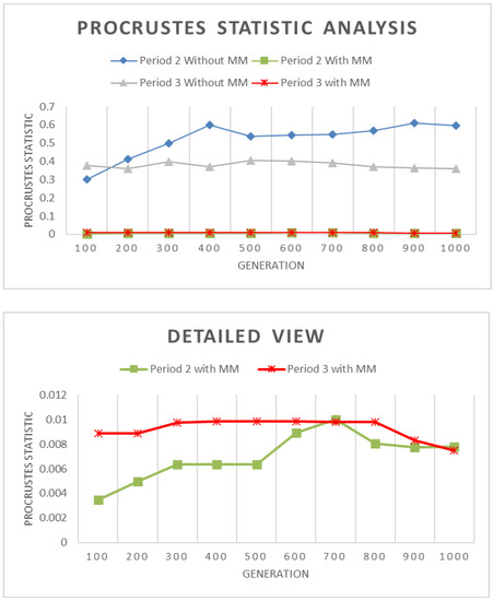
Figure 12.
Procrustes analysis results.
3.4. Further Optimization
In our experimental results, we found that, by considering all possible starting periods (by spending n times the time that starts from the first period, where n is the number of periods), the system can look for the best period to start with, i.e., it is not always needed to start with the first period. Figure 13 shows the score (cost) in each period (two months) in 2000, and as we can see, the best score with the backward method (i.e., to consider all the possible cases) is in the fourth period. Figure 14 shows the comparisons in three different years (2000, 2004 and 2008) with and without the backward approach to explain how the best score is essential to get the best period to start with.
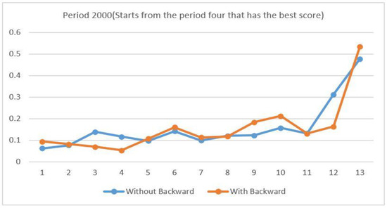
Figure 13.
The scores with and without backward to find the best period to start with.
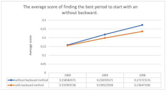
Figure 14.
Comparison of an average score with and without backward in three different years.
4. Discussion
Through our generated animation, we observed that, throughout the years, adventure and action games have never ceased to be released. They dominate most of the time, even until 2019. We observed that most of the adventure games are Japanese titles, and Japan seems to contribute to most of the video game development and, thus, why adventure games are always released each month. In early 1998, most of the released games were action and fighting games like Street Fighter and Mortal Kombat, as they were popular in arcades. There were also a lot of miscellaneous games released, such as chess or a compilation of games. During the period from 2000 to 2008, adventure and action games dominated where action games were mostly first-person shooter, such as Counter Strike, Doom and the Call of Duty series. From 2007 to 2011, there was a rise in puzzle games, and they were mostly of hidden object games by developers such as PopCap studios, BigFish games or GameHouse, which also led the trend of puzzle games such as Mystery Case File, Zuma, Diner Dash and Bejeweled becoming popular among PC users. During 2010–2012, role playing games also seemed to rise with the hype of famous role playing game titles such as Diablo III, The Witcher 2 and the Assassin Creed series. Lastly, during 2015–2018, action games kept rising and dominated most of the time. Although our dataset did not include neurogaming, it seems as though it may be more popular in the future, because a potential user, a player, may interfere with the world of the game without using traditional peripheral devices such as a keyboard, mouse or a joystick [20].
Based on the experiment results, we can also conclude that considering the mental map weight since the start of the GA generations gives the best preservation, as our GA is better at preserving the mental map by constraining the nodes to their previous positions. We also proved that combining Path Relinking (PR) with GA is not as good as combining PR with Tabu Search through our experiments. However, using PR indeed gives a considerably faster convergence rate but not a better result. As our implementations are web-based systems using the usual front-end and back-end approaches, most of the calculations are done in Node.js. However, Node.js is not optimized for this kind of processing like C++ or python is, resulting in a slow calculation process and computing time. Another solution is to find a way to process them in parallel through the GPU, similar to the works of Qu et al. [9], to reduce the calculation time needed. It is also hard to tinker with too many nodes, even with our simplification algorithm, because most of the results are not informative enough. Compared with the cases of lesser nodes, more nodes means more edges, and D3.js cannot handle drawing too many edges. We also observed a slow computing time calculating our proposed fitness value, because the Greadability.js library calculates edge crossing and angular resolution for our system. With more edges, the processing times increase exponentially, and this is a problem that every graph-drawing algorithm encounters. Graph features such as the node’s color and size may also affect a user’s mental map.
5. Conclusions
In this research, we developed a web-based application that can produce and show the smooth animation of multiple undirected graphs. We proposed a mental map-preserving algorithm for an undirected graph using a GA that can be applied to all datasets as long as the relationship can be calculated and develop a web-based application for users to control and create the animation of graphs. Our research concluded that a smoother animation can be achieved by preserving a user’s mental map, and the information was indeed better preserved throughout the animation. Future research could be done to reduce the calculation time and to use more efficient programming languages such as Python to help improve the mental map preservation, especially when too many nodes are involved.
Author Contributions
Conceptualization, M.D. and C.-K.Y.; methodology, M.D.; software, E.A.; validation, M.D., C.-K.Y. and E.A.; formal analysis, M.D.; investigation, M.D.; resources, M.D.; data curation, M.D.; writing—original draft preparation, E.A. and M.D.; writing—review and editing, C.-K.Y.; visualization, M.D. and E.A.; supervision, C.-K.Y.; project administration, M.D. and C.-K.Y. and funding acquisition, C.-K.Y. All authors have read and agreed to the published version of the manuscript.
Funding
This research was funded by the Ministry of Science and Technology, Taiwan, with grant numbers MOST 106-2221-E-0110148-MY3, MOST 107-2218-E-011-012, MOST 108-2218-E-011-021, MOST 109-2221-E-011-133 and MOST 109-2218-E-011-007.
Conflicts of Interest
The authors declare no conflict of interest.
References
- Kamada, T.; Kawai, S. An algorithm for drawing general undirected graphs. Inf. Process. Lett. 1989, 31, 7–15. [Google Scholar] [CrossRef]
- Fruchterman, T.M.J.; Reingold, E.M. Graph drawing by force-directed placement. Softw. Pract. Exp. 1991, 21, 1129–1164. [Google Scholar] [CrossRef]
- Davidson, R.; Harel, D. Drawing graphs nicely using simulated annealing. ACM Trans. Graph. 1996, 15, 301–331. [Google Scholar] [CrossRef]
- Zhang, Q.-G.; Liu, H.-Y.; Zhang, W.; Guo, Y.-J. Drawing Undirected Graphs with Genetic Algorithms. In International Conference on Natural Computation; Springer: Berlin/Heidelberg, Germany, 2005; pp. 28–36. [Google Scholar]
- Rosete-Suárez, A.; Ochoa-Rodríguez, A.; Sebag, M. Automatic graph drawing and Stochastic Hill Climbing. In Proceedings of the 1st Annual Conference on Genetic and Evolutionary Computation, Orlando, FL, USA, 13–17 July 1999; Volume 2, pp. 1699–1706. [Google Scholar]
- Pinaud, B.; Kuntz, P.; Lehn, R. Dynamic Graph Drawing with a Hybridized Genetic Algorithm. In Adaptive Computing in Design and Manufacture VI; Springer: London, UK, 2004; pp. 365–375. [Google Scholar]
- Barreto, A.M.S.; Barbosa, H.J.C. Graph layout using a genetic algorithm. In Proceedings of the Sixth Brazilian Symposium on Neural Networks, Rio de Janeiro, Brazil, 22–25 November 2000; Volume 1, pp. 179–184. [Google Scholar]
- Branke, J.; Bucher, F.; Schmeck, H. Using Genetic Algorithms for Drawing Undirected Graphs. In Proceedings of the Third Nordic Workshop on Genetic Algorithms and their Applications, Helsinki, Finland, 18–22 August 1997. [Google Scholar]
- Qu, J.; Liu, X.; Sun, M.; Qi, F. GPU-Based Parallel Particle Swarm Optimization Methods for Graph Drawing. Discret. Dyn. Nat. Soc. 2017, 2017, 1–15. [Google Scholar] [CrossRef]
- Dib, F.K.; Rodgers, P. Graph drawing using tabu search coupled with path relinking. PLoS ONE 2018, 13, e0197103. [Google Scholar] [CrossRef] [PubMed]
- Eades, P.; Lai, W.; Misue, K.; Sugiyama, K. Preserving the mental map of a diagram. In Proceedings of the Compugraphics ’91, Sesimbra, Portugal, 16–20 September 1991; pp. 24–33. [Google Scholar]
- Paszkiel, S.; Szpulak, P. Methods of Acquisition, Archiving and Biomedical Data Analysis of Brain Functioning, Biomedical Engineering and Neuroscience; Book Series: Advances in Intelligent Systems and Computing; Springer: Cham, Switzerland, 2018; pp. 158–171. [Google Scholar]
- Rafelsberger, W.M. Interactive Visualization of Evolving Force-Directed Graphs. In International Conference of Design, User Experience, and Usability; Springer: Berlin/Heidelberg, Germany, 2013; pp. 553–559. [Google Scholar]
- Lee, Y.-Y.; Lin, C.-C.; Yen, H.-C. Mental map preserving graph drawing using simulated annealing. In Proceedings of the 2006 Asia-Pacific Symposium on Information Visualisation, Tokyo, Japan, 1–3 February 2006; Volume 60, pp. 179–188. [Google Scholar]
- Resende, M.G.C.; Ribeiro, C.C. Path-relinking. In Optimization by GRASP: Greedy Randomized Adaptive Search Procedures; Springer: New York, NY, USA, 2016; pp. 167–188. [Google Scholar]
- Bridgeman, S.; Tamassia, R. A User Study in Similarity Measures for Graph Drawing. In Graph Algorithms and Applications 3; World Scientific: Singapore, 2004; pp. 225–254. [Google Scholar]
- Gower, J.C. Generalized procrustes analysis. Psychometrika 1975, 40, 33–51. [Google Scholar] [CrossRef]
- Kravchenko, O. (Generalized) Procrustes Analysis with Python/NumPy. Available online: https://medium.com/@olga_kravchenko/generalized-procrustes-analysis-with-python-numpy-c571e8e8a421 (accessed on 1 December 2020).
- Sphinx. Scipy.Spatial.Procrustes. Available online: https://docs.scipy.org/doc/scipy/reference/generated/scipy.spatial.procrustes.html (accessed on 1 November 2020).
- Paszkiel, S. Computer Game in UNITY Environment for BCI Technology, Analysis and Classification of Eeg Signals for Brain-Computer Interfaces; Book Series: Studies in Computational Intelligence; Springer: Cham, Switzerland, 2020; pp. 101–110. [Google Scholar]


Publisher’s Note: MDPI stays neutral with regard to jurisdictional claims in published maps and institutional affiliations. |
© 2021 by the authors. Licensee MDPI, Basel, Switzerland. This article is an open access article distributed under the terms and conditions of the Creative Commons Attribution (CC BY) license (https://creativecommons.org/licenses/by/4.0/).