Abstract
This paper proposes a method to detect the defects in the region of interest (ROI) based on a convolutional neural network (CNN) after alignment (position and rotation calibration) of a manufacturer’s headlights to determine whether the vehicle headlights are defective. The results were compared with an existing method for distinguishing defects among the previously proposed methods. One hundred original headlight images were acquired for each of the two vehicle types for the purpose of this experiment, and 20,000 high quality images and 20,000 defective images were obtained by applying the position and rotation transformation to the original images. It was found that the method proposed in this paper demonstrated a performance improvement of more than 0.1569 (15.69% on average) as compared to the existing method.
1. Introduction
Manufacturing systems are progressing with the advancements in the industry. The core technologies used in manufacturing systems can be classified into machine vision technology, industrial robot control technology, industrial PC technology, programmable logic controller (PLC) technology, and sensor technology. Among them, machine vision technology is thought to be an important technology, able to either reduce production costs or improve productivity [1,2,3,4,5,6]. In this paper, we adopt machine vision technology to detect incorrect parts (called defects) occurring during the assembly process.
The parts assembly process is an important factor in lowering the defect rate of finished products because, if a defective part is used in a finished product, it is seen as a defect of the finished product rather than as a defect of the part itself. The defect rate may be affected by a worker’s ability and work environment since the worker determines the inputs and assembles the components of the part. Consequently, the defect rate may decrease if the product is assembled by a skilled worker. As such, automation is also a crucial factor in reducing the defect rate of finished products during the assembly process [7,8].
Machine vision technology can be classified into two categories based on “after” and “before” parts production. The first is a technology to detect defects after parts production, and the second is a technology to classify components of production parts for the purpose of improving the work efficiency of workers before parts production. One of the technologies used in both categories is alignment calibration technology. Although it is a technology that senses the angle and position of a product by using a mark engraved on it or a unique pattern on the product itself, there are cases in which unique patterns and marks cannot be used, owing to the structural characteristics of the production parts (such as automotive parts).
Accuracy and processing speed are important factors in the process of automotive parts classification. Accuracy refers to a metric showing how well the system distinguishes the vehicle type by extracting features after calibrating the alignment of the input parts. The processing speed is the time required to distinguish the vehicle type. In this context, this paper proposes a method for classifying vehicle types by measuring the size of the parts after calibrating their alignment and after improving the processing speed of vehicle classification by applying CPU-based parallel processing. In addition, this paper proposes a method to distinguish defects based on a convolutional neural network (CNN) for accuracy.
Conventional alignment calibration techniques include a line detection method [9], an integral histogram method [10,11], and a projection-based integral histogram method [1]. The line detection method calibrates the alignment of a part by detecting a line, which is a characteristic of the part. Although alignment can be quickly calibrated using a line of the part when there is a straight line in a section of an image, there may be alignment errors in the case of vehicle headlights because they are configured with curved surfaces. Consequently, processing time and costs may increase. The integral histogram method detects marks, such as circles and crosses, by applying integral, histogram-based template matching. In this method, good detection performance cannot be expected if there is no mark on the part. Although improved integral histogram methods incorporate a projection-based integral histogram method, a unique pattern cannot be used because of the characteristics of vehicle headlight parts. These conventional techniques are difficult to apply for vehicle headlights and, thus, in this paper, a new alignment calibration technique using a major axis of an object is used.
To detect incorrect parts of an input headlight, after calibrating their alignment, the system distinguishes the vehicle type, which requires a quick processing time. To complete this, in this paper, a method for distinguishing vehicle types by the size of the parts is proposed, where its processing speed is improved by applying CPU-based parallel processing. In addition, this paper proposes a method to determine defect or not based on a convolutional neural network (CNN) for accuracy improvement. The proposed method is similar to the method of [12] where the existence of a defect or lack thereof is judged by the similarity (correlation coefficient, etc.) of an inspection target with the template image. The criteria for determining defect or not is defined by the operator in [12]. However, in this paper, the classification model is automatically illustrated from raw images by VGG19, which is a convolutional neural network. This means the system does not need to define a similar measurement and its threshold manually.
The structure of this paper is as follows. Section 2 explains the overall system structure of the technology applied. Section 3 describes the proposed vehicle part alignment calibration and the CNN-based defect detection method. Section 4 discusses the experimental results on the defect detection performance between the proposed method and the existing method, and Section 5 concludes this paper.
2. System Configuration
The traditional work environment for manufacturing a conventional vehicle headlight is shown in Figure 1a. It is an environment in which several workers assemble two or more headlight parts in one conveyor system. The worker determines the vehicle type of the headlight and selects the parts to be assembled. However, in the case of some parts, the structure of the headlights is similar, as shown in Figure 1b,c, which may result in errors in the assembly process.
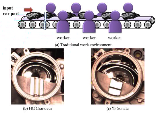
Figure 1.
Traditional work environment and headlight images.
The method proposed in this paper automatically determines the defects for different types of parts, as shown in Figure 2. The alignment is calibrated by extracting the features of the vehicle headlight when the vehicle headlight is first input to the system, and whether the headlight is defective or not is determined based on the CNN after detecting the region of interest (ROI).
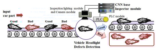
Figure 2.
CNN-based vehicle headlight defects of the detection system structure.
The classifier system for different part types consists of an inspector module, PLC module, inspection lighting module, and camera module. The functions of each part type are as follows.
- Inspection lighting module: This module controls the amount of light for image shooting when a vehicle headlight is input into the inspection region. It is controlled by the inspector module.
- Camera module: When a vehicle headlight is input into the inspection region for detecting defects, the part is photographed by the camera module and the captured image is transmitted to the inspector module.
- Inspector module: The inspector module receives vehicle headlight images from the camera module, detects defects in the headlight area of the received images, and transmits information on the presence of defects to the PLC.
- PLC module: The PLC module receives information regarding the presence of defective vehicle headlights from the inspector module and classifies vehicle headlights as superior or inferir based on the presence of defects.
3. Method for Detecting Defective Vehicle Headlight Parts
In order to judge the defect, the recipe must be saved by executing the system first. The recipe (information on inspection regions, camera settings, lighting brightness settings, and so on) of a vehicle type is saved by the recipe save module in Figure 3 after executing the start module, which checks the status of the equipment in terms of system operation and sets the motor’s default position. After saving the recipe, the system is run again to perform the defect determination process. In this process, the start module is executed first through which a vehicle model (or type) for inspection is determined and then the motor is moved to the inspection position of the vehicle type. Then, some values for the camera and the light settings are loaded from the recipe load module and transferred. Afterward, the defect is judged by the normal operation module. The normal operation module is a module related to the actual model classification and inspection, which returns the inspection result and stores it for a history search in the database.
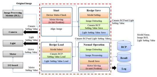
Figure 3.
Program structure.
The proposed method for detecting whether headlight components are defective is comprised of two processes. The first process is the inspection reference information setting process, which sets the inspection region (ROI) after position calibration of the acquired image. The structure of a vehicle headlight is different for each vehicle type, and the position, number, and size of the inspection regions are different. Therefore, in the first process, the worker designates the position and size of the part to be inspected and saves the position and size of the inspected region in the database. The second process determines the presence of defects within ROIs based on the CNN after position calibration of the acquired image, as shown in Figure 4.
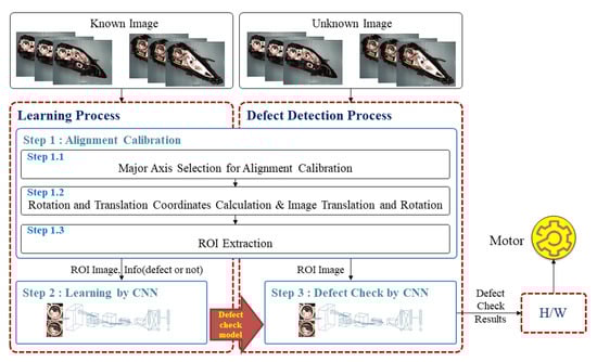
Figure 4.
Structure of the defect checker module.
3.1. Alignment Calibration Using Major Axis Coordinates (Step 1)
The processing of the major axis coordinate search step for alignment calibration consists of a total of four steps. The first step is the likelihood-based color model transformation used in the particle filter [13,14,15]. The second step is the object acquisition, object hole removal, and object major axis coordinate search. The third step is the translation and rotation transformation. Finally, the fourth step is the obtainment of ROIs using the major axis of the object.
3.1.1. Likelihood-Based Color Model Transformation
When a vehicle headlight image is captured using the inspection lighting (Figure 5a), there is a shadow due to the structure of the headlight. Thus, the color distribution in the histogram is skewed to one side (Figure 5d) when binarization is performed based on the gray-scale image [16]. Consequently, the interval to be set as the threshold value narrows (Figure 5d ①). Moreover, three threshold values need to be selected when using the hue-saturation-value (HSV) model in order to minimize the influence of light. Only one threshold can be used instead of three since the likelihood and normalization are applied after changing the red-green-blue (RGB) model to the HSV model to minimize the influence of light. As such, a wider threshold setting interval than the gray-scale, image-based setting interval should be used in the proposed method.
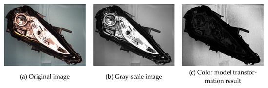
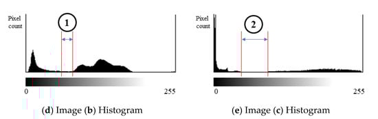
Figure 5.
Comparison of a likelihood-based color model image with a gray-scale color model image.
The applied likelihood is shown in Equation (1). The likelihood value is calculated using the HSV value of the sampling coordinate and the HSV value of the input image. Normalization is applied by employing Equation (2) after calculating the likelihood value. The result of this step is shown in Figure 5c, and the threshold setting interval is shown in Figure 5e ②.
where denotes the likelihood result value of the pixel, denotes the hue value of the sampling coordinate , denotes the hue value of the image coordinate , denotes the normalized value of the image coordinate , and denotes the height and width of the input image.
3.1.2. Object Acquisition and Object Major Axis Coordinate Search
After binarization, the object is acquired—as shown in Figure 6b—by applying a flood fill [17] to remove the noise in the background, as shown in Figure 6a. The reference coordinates of the inspection target are required in order to apply the flood fill, and the worker inputs these directly when setting the recipe. There is an internal hole in a headlight, which needs to be removed since it may affect feature extraction. To this end, the internal hole is removed using the same method as extracting the background, and OpenMP is used to shorten the operating time.
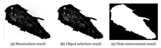
Figure 6.
Object detection.
The hole removement process is as follows, of which the result is shown in Figure 6c.
① Object acquisition using flood fill.
② Change the value of the image border to any value other than 0 and 1.
③,④ Initiate parallel processing for the top and bottom. Each processor changes the current pixel value to the border value if the current pixel value is 1 and the previous pixel value is the border value. No changes are made to the pixel value if the current pixel value is 0.
⑤ Change the pixel value to 1 if the current pixel value is 0 or 1.
⑥ Obtain the final result.
In terms of the major axis coordinate search of the object, the distance from the center of the object to the coordinate of the object with left and right pixel values of 1 is calculated, as shown in Figure 7a, after calculating the center coordinate of the object using its upper left (e.g., ⓐ) and lower right (e.g., ⓑ) coordinates, as shown in Figure 7b. The left and right major axis coordinates of the object are obtained by finding the coordinates with the greatest distance value, among the calculated distances, to the left and right pixels. This process is expressed by Equations (3) and (4).
where and denote the left border ()/right border () coordinates of the object, and denote the coordinates of the center of the object : , , and denote the coordinates of a pixel with a value of 1 among the left-end and the right-end pixels of the object, respectively.
Figure 7.
Major axis coordinate search.
3.1.3. Image Translation and Rotation
The image translation and rotation method comprise a total of three steps. The first step is the calculation of the rotation angle and the translation coordinate. The second step is the image translation transformation, and the last step is the image rotation transformation. In the first step, the translation coordinate is the distance from the center of the major axis to the image center coordinate, and the rotation angle is the angle at which the major axis will rotate. The translation coordinates are calculated by first obtaining the center coordinates (()/2, (where and are the coordinates of the left and right end points of the major axis—and then finding the difference between this central coordinate and the image central coordinate, as shown in Figure 8a. The angle at which the image is to be rotated is calculated using the following equation , as shown in Figure 8b.
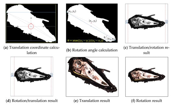
Figure 8.
Image translation and rotation.
In the second step, image translation and rotation are applied by using the rotation angle and the translation coordinate obtained in the calculation step. The image translation transformation is applied first, since—although the translation coordinate calculated earlier is affected by the image rotation when the image rotation transformation is initially applied—the rotation angle calculated earlier is not affected by the image translation when the image translation transformation is first applied. In other words, although the rotation transformation leaves the distance to the left and right unchanged after the image translation transformation, as shown in Figure 8c ① and ②, the rotation transformation is applied (as shown in Figure 8f) after employing the translation transformation (as shown in Figure 8e). This is because the distance to the left and right of the translation transformation after image rotation transformation is different (as shown in Figure 8d ① and ②).
3.1.4. ROI Designation and Acquisition
The image provided to the worker for the purpose of setting the coordinates of the ROI is not the raw image acquired from the camera, but an image from which holes have been removed after completion of the normalization process of position calibration. If an image that has not completed the normalization process is used, the position and angle may change depending on the environment in which the image is acquired, and there may be false detection problems when determining defects. To this end, this paper provides the worker with an image processed with normalization to set the inspection region.
The image from which the surrounding background has been removed is provided to the worker, as shown in Figure 9a, and the coordinates are set to the coordinates with the surrounding background removed. The ROI information is managed by grouping the start coordinates of the inspection region, the size information of the region, and the reference image into one set.
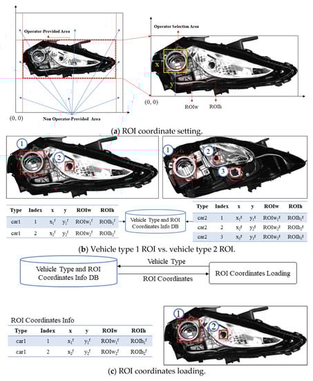
Figure 9.
ROI coordinates setting and loading.
Since the structure of the headlights for each vehicle type is different, the location of the inspection region, the number of inspection targets, and the size of the inspection region are configured differently, as shown in Figure 9b. Therefore, the size or the number of the region and position coordinates cannot be designated identically when setting and storing the inspection region. In this study, the database and input screen are configured to individually designate and manage the inspection region information and reference images for each model.
For the purpose of detecting defects, the inspection region information for an ROI is searched and loaded from the database based on the model classification information, as shown in Figure 9c. The inspection region information contains inspection region coordinates, of which each set has a reference image, index, start coordinate, and inspection region size, and is transmitted to detect the presence of defects, where n denotes the number of inspection regions set by the worker in the inspection region coordinate setting step.
3.2. CNN-Based Training for Detecting Defects (Step 2)
The size of the ROI for detecting defects is different for each inspection region, as shown in Figure 9. Therefore, an image size conversion process is required to apply the previously proposed CNNs of various structures (ReNet-5, AlexNet, GooLeNet, REsNet, VGG19, etc. [18,19]) to an ROI image. The feature map size of the input layer of ReNet-5 is 32 × 32 of which the depth is 1. In the case of AlexNet, the feature map size is 227 × 227, and the depth is 3. In the cases of GooLeNett, REsNet, and VGG19, the feature map size is 224 × 224, and the depth is 3. Therefore, the image size of the ROI needs to be changed to fit the input layer. In this study, VGG19 was used, and the image size of the ROI was changed to fit the input layer of VGG19, as shown in Figure 10. Among the verified CNNs, the VGG19 has the advantage of a simple structure and good performance for classification. In addition, it can be easily applied to field applications. Therefore, the VGG19 was used in this paper.
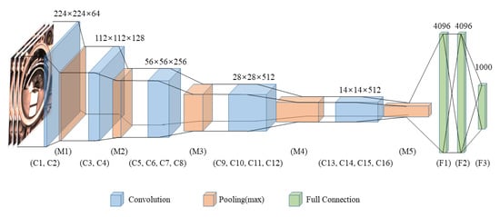
Figure 10.
VGGNet-19 structure.
The detailed structure of VGG19 includes a feature size and stride of the convolution layer of 3 × 3 and 1, respectively, and the padding is configured to be the same as shown in Table 1, in which a CNN model for detecting defects is built, and used to detect defects in parts.

Table 1.
VGGNet-19 structure details (ReLu(Rectified Linear Unit)).
3.3. CNN-Based Defect Detection (Step 3)
It was found that the ROI position and size to be detected for defects were different depending on the vehicle type, and the ROI size was different for the same vehicle type. Therefore, the CNN model was constructed for each ROI of the vehicle type, and the presence of defects (Good = 0, NG = 1) was detected for each model, as shown in Figure 11. Finally, the vehicle headlight was determined to be good after tallying the result of each model if the sum is zero, and, as NG, if the result’s sum did not equal zero.
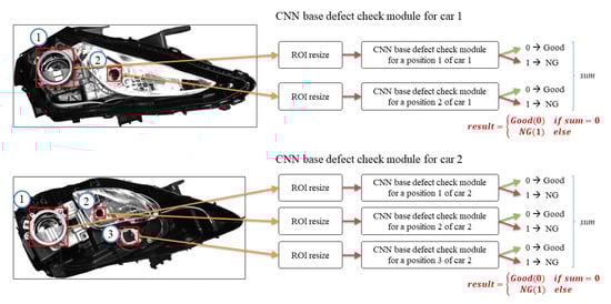
Figure 11.
CNN-based defects check module structure.
4. Experimental Section
4.1. Experimental Environment and Data Acquisition
For the purpose of this experiment, the hardware for detecting defects was constructed, as shown in Figure 12. The lighting used for image shooting was a flat LED light with a diffuser plate attached to the camera and mounted in the center. The images were acquired by placing the camera, lens, and light vertically, and shooting from above. The camera and lens specifications are summarized in Table 2. One sample was used for each of the two vehicle types during image acquisition, and 100 images were acquired for each, thereby, acquiring a total of 200 images.
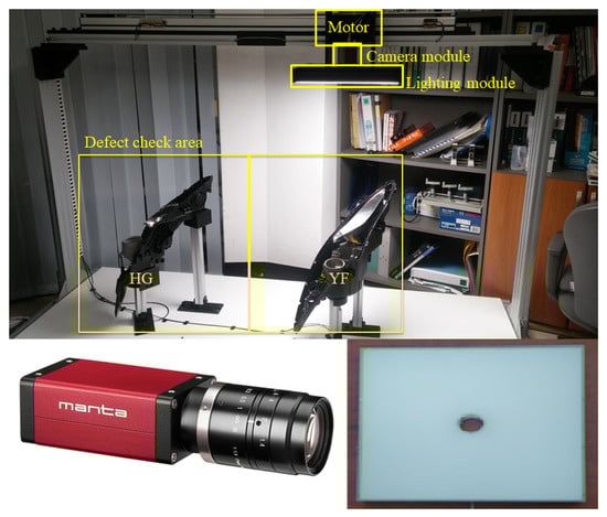
Figure 12.
Image shooting environment.
Table 2.
Camera and lens specifications.
The 100 images used to train the CNN could be said to be a small quantity of data. Hence, the ROI image for training was obtained by applying rotation and translation transformation to the image that had been aligned in step 1. The image rotation and translation transformation methods were randomly applied in the range of −5° to +5°, and −10 pixels to +10 pixels up, down, left, and right. A total of 200 high quality images and 200 defective images were secured based on one image. In other words, there were a total of 40,000 images for each vehicle type, of which 20,000 images could be said to be of high quality (Table 3). The criterion for defective and high quality was defined as high quality when the position was close to the ROI, as shown in Figure 13a, and, as a defect, when it was far from the ROI, as shown in Figure 13b.
Table 3.
Total data set.
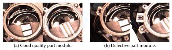
Figure 13.
Sample of high vs. defective parts module.
4.2. CNN-Based Defect Detection Experiment and Results
The defect detection experiment based on the CNN was divided into three experiments. The first was a two-class detection experiment, the second was a three-class detection experiment, and the last was a four-class detection experiment. The two-class detection experiment was divided into three sub-experiments in which the first was a two-class classification for high quality and defects of the YF model, the second sub-experiment was a two-class classification for high quality and defects of the HG model, and the last sub-experiment was a two-class classification for the detection of HG and YF models. The three-class detection experiment was divided into two sub-experiments, in which the first sub-experiment was a three-class classification including YF defects in the HG and YF model classification, and the second sub-experiment was a three-class classification including HG defects in the HG and YF model classification. Finally, the four-class detection experiment was a four-class classification including both high quality images and defective images of the YF model as well as high quality images and defective images of the HG model as a single experiment.
As for the performance verification method for each experiment, 80% of the data were randomly used as training data and 20% of the data were used as test data (Table 4).
Table 4.
Test and training dataset for the experiment.
In the E. 1 (two-class) detection experiment, which was the first experiment, the result of Sub E. 1 showed an accuracy of 0.97(=97%) or higher (after 500 Step), regardless of the training steps for both the training set and the test set, as shown in Figure 14a. The highest accuracy in the training step was 1.00 for both the training set and the test set, and the lowest accuracy was 0.9797 for the training set and 0.9995 for the test set. The results of Sub E. 2 showed an accuracy of 0.98 or higher, as shown in Figure 14b. The highest accuracy in the training step was 1.00 for the training set and 1.00 for the test set, and the lowest accuracy was 0.9818 for the training set and 0.9946 for the test set. Finally, the result of Sub E. 3 showed an accuracy of 0.98 or higher, as shown in Figure 14c. The highest accuracy in the training step was 1.00 for the training set and 1.00 for the test set, and the lowest accuracy was 0.9848 for the training set and 1.00 for the test set.
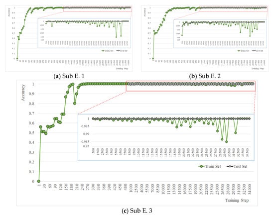
Figure 14.
Accuracy of experiment 1 (two-class).
In the E. 2 (three-class) detection experiment, which was the second experiment, the result of Sub E. 1 showed an accuracy of 0.97 or higher (after 500 steps) regardless of the training step for both the training set and the test set, as shown in Figure 15a. The highest accuracy in the training step was 1.00 for both the training set and the test set, and the lowest accuracy was 0.9717 for the training set and 0.9978 for the test set. In addition, the results of Sub E. 2 showed an accuracy of 0.9894 or higher, as shown in Figure 15b. The highest accuracy in the training step was 1.00 for the training set and 0.9999 for the test set, and the lowest accuracy was 0.9894 for the training set and 0.998 for the test set.
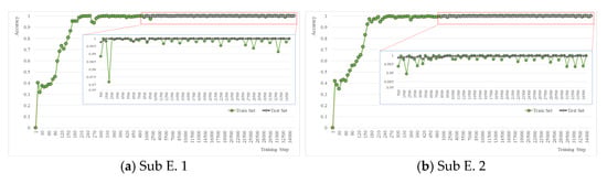
Figure 15.
Accuracy of experiment 2 (three-class).
The result of E. 3 (4-class), which was the third experiment, showed an accuracy of 0.98 or higher (after 500 steps) regardless of the training step for both the training set and the test set, as shown in Figure 16. The highest accuracy in the training step was 1.00 for both the training set and the test set, and the lowest accuracy was 0.9909 for the training set and 0.9856 for the test set.
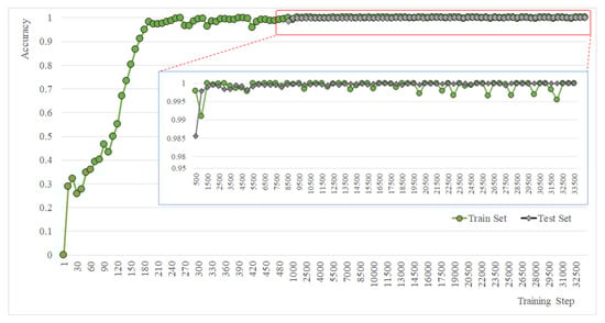
Figure 16.
Accuracy of experiment 3 (four-class).
4.3. Performance Comparison between the Proposed Method and the Existing Method
To measure the objective performance of the proposed method, it was compared with the existing method [12], with the reference image being randomly set in the same way as the existing method to compare performance. The reference value to classify high quality images and defects required for the existing method was set to “less defects.” In addition, because the existing method was a two-class classification for good quality and defects, it was compared with the performance of E. 1 (2-class), a two-class classification experiment of the proposed method (Table 4).
For the YF model, which was the first experiment, the results of detecting high quality images and defective images are shown in Figure 17 E1S1. The proposed method showed a classification performance of 1.00, whereas the existing method showed a classification performance of 0.9948 (TM_SQDIFF_NORMED). For the HG model, which was the second experiment, the results of detecting high quality images and defective images are shown in Figure 17 E1S2. The proposed method showed a classification performance of 1.00, whereas the existing method showed a classification performance of 0.9363 (TM_CCORR). For the HG and YF model detection, which was the final experiment, the results are shown in Figure 17 E1S3 (by YF and HG). The proposed method showed a classification performance of 1.00, whereas the existing method showed a classification performance of 0.6731 (by YF, TM_CCORR) and 0.7683 (by HG, TM_CCORR). As shown in the results of this experiment, it was found that the performance of the method proposed in this paper exhibited an improvement of 0.1569 (average) when compared with the existing method.
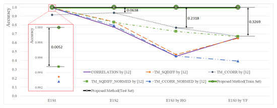
Figure 17.
Classification performance (proposed method vs. existing method).
5. Conclusions
A method to detect defects in products was proposed in this paper based on a CNN after calibrating the alignment, in order to reduce the defects depending on the workers’ ability and work environment when manually assembling the components. The defect detection performance was compared with the existing defect detection method to analyze objective performance. It was found that the proposed method showed a performance improvement of more than 0.1569 (15.69% on average) as compared to the existing method.
In this paper, the hardware was a beta version, which is an environment for algorithm and system development. Thus, the performance of the proposed method will need to be verified in a real hardware system of the Smart Factory.
Author Contributions
Conceptualization, B.-M.K. and C.-B.M.; Formal analysis, B.-M.K.; Design and implementation, C.-B.M. and J.-Y.L.; experiment, C.-B.M.; writing—review and editing, D.-S.K. and B.-M.K. All authors have read and agreed to the published version of the manuscript.
Funding
This research was supported by the Basic Science Research Program through the National Research Foundation of Korea (NRF) funded by the Ministry of Education (NRF-2020R1F1A104833611). This research was supported by the MSIT (Ministry of Science and ICT), Korea, under the Grand Information Technology Research Center support program (IITP-2021-2020-0-01612) and supervised by the IITP (Institute for Information & communications Technology Planning & Evaluation).
Institutional Review Board Statement
Not applicable.
Informed Consent Statement
Not applicable.
Data Availability Statement
The data presented in this study are available on request from the corresponding author.
Conflicts of Interest
The authors declare no conflict of interest.
References
- Moon, C.B.; Kim, H.S.; Kim, H.-Y.; Lee, D.W.; Kim, T.-H.; Chung, H.; Kim, B.M. A Fast Way for Alignment Marker Detection and Position Calibration. KIPS Trans. Softw. Data Eng. 2016, 5, 35–42. [Google Scholar] [CrossRef]
- Viola, P.; Jones, M.J.; Snow, D. Detecting Pedestrians using Patterns of Motion and Appearance. Int. J. Comput. Vis. 2005, 63, 153–161. [Google Scholar] [CrossRef]
- Felzenszwalb, P.F.; Girshick, R.B.; McAllester, D.; Ramanan, D. Object Detection with Discriminatively Trained Part-based Models. IEEE Trans. Pattern Anal. Mach. Intell. 2010, 32, 1627–1645. [Google Scholar] [CrossRef] [PubMed]
- Stauffer, C.; Grimson, W.E.L. Learning Patterns of Activity using Real-time Tracking. IEEE Trans. Pattern Anal. Mach. Intell. 2000, 22, 747–757. [Google Scholar] [CrossRef]
- Krizhevsky, A.; Sutskever, I.; Hinton, G.E. Imagenet Classification with Deep Convolutional Neural Networks. Adv. Neural Inf. Process. Syst. 2012, 25, 1097–1105. [Google Scholar] [CrossRef]
- Lu, C.-C.; Juang, J.-G. Robotic-Based Touch Panel Test System Using Pattern Recognition Methods. Appl. Sci. 2020, 10, 8339. [Google Scholar] [CrossRef]
- Moon, C.B.; Ahn, Y.H.; Lee, H.-Y.; Kim, B.M.; Oh, D.-W. Implementation of Automatic Detection System for CCFL’s Defects based on Combined Lighting. J. Korea Soc. Ind. Inf. Syst. 2010, 15, 69–81. [Google Scholar]
- Matuszek, J.; Seneta, T.; Moczała, A. Assessment of the Design for Manufacturability Using Fuzzy Logic. Appl. Sci. 2020, 10, 3935. [Google Scholar] [CrossRef]
- Kwon, S.J.; Park, C.; Lee, S.M. Kinematics and control of a visual alignment system for flat panel displays. J. Inst. Control Robot. Syst. 2008, 14, 369–375. [Google Scholar]
- Park, C.S.; Kwon, S.J. An efficient vision algorithm for fast and fine mask-panel alignment. In Proceedings of the 2006 SICEICASE International Joint Conference (SICE-ICCAS 2006), Busan, Korea, 18–21 October 2006; pp. 1461–1465. [Google Scholar]
- Jung, U.-K.; Moon, C.B.; Lee, H.-Y.; Kim, B.M.; Yang, H.S. Preprocessing Algorithm for Detecting CCFL Defects. In Proceedings of the 2009 Conference on Korean Institute of Information Scientists and Engineers, Seoul, Korea, 27 November 2009; Volume 36, pp. 359–362. [Google Scholar]
- Kim, K.H.; Moon, C.B.; Kim, B.M.; Oh, D.H. Inspection of Vehicle Headlight Defects. J. Korea Ind. Inf. Syst. Res. 2018, 23, 87–96. [Google Scholar]
- Condensation. Available online: http://opencv.jp/sample/estimators.html (accessed on 4 January 2021).
- Particle Filter Tracking in Python. Available online: https://www.slideshare.net/kohta/particle-filter-tracking-in-python (accessed on 4 January 2021).
- Pulli, K.; Baksheev, A.; Kornyakov, K.; Eruhimov, V. Realtime Computer Vision with OpenCV; ACM Queue: New York, NY, USA, 2012. [Google Scholar]
- Hwang, S. Image Processing Programming by Visual C++; Hanbit Publishing Network: Seoul, Korea, 2007. [Google Scholar]
- Shane, T. Applied Computer Science, 2nd ed.; Springer: Berlin/Heidelberg, Germany, 2016; p. 158. [Google Scholar]
- Kim, B.M.; Lee, J.Y.; Moon, C.B. Deep Learning in Practice; Hongreung Publishing Company: Seoul, Korea, 2020. [Google Scholar]
- Szegedy, C.; Liu, W.; Jia, Y.; Sermanet, P.; Reed, S.; Anguelov, D.; Rabinovich, A. Going Deeper with Convolutions. In Proceedings of the IEEE Conference on Computer Vision and Pattern Recognition, Columbus, OH, USA, 23–28 June 2014; pp. 1–9. [Google Scholar]


Publisher’s Note: MDPI stays neutral with regard to jurisdictional claims in published maps and institutional affiliations. |
© 2021 by the authors. Licensee MDPI, Basel, Switzerland. This article is an open access article distributed under the terms and conditions of the Creative Commons Attribution (CC BY) license (https://creativecommons.org/licenses/by/4.0/).