Abstract
In this study, the post-yield load-displacement relationships of precast composite beams with various boundary conditions were predicted based on strength degradation data. The aim of this study was to explore the post-yield hysteretic structural behavior of precast composite concrete beams based on stiffness degradation, which was calculated by normalizing effective stiffness with respect to stiffness at the yield limit state. The influence of degradation of the effective stiffness on the post-yield behavior of the specimens was investigated with extensive test data gathered using gauge measurements. The hysteresis behavior, determined from cyclic tests of full-scale composite specimens under the various boundary conditions, was used to predict the post-yield deflection of the composite beams. This paper collected post-yield test data for 13 specimens, including five pre-stressed specimens, to investigate the influence of pre-stressing forces on the post-yield characteristics of steel-concrete composite beams. The prediction of post-yield load-displacement relationships of the composite beams was based on six steps and matched well with test data, verifying the proposed analytical procedures for estimating post-yield performance. The post-yield load-displacement relationships of precast composite concrete beams were satisfactorily predicted by the simplified but convenient method.
1. Introduction
Steel-reinforced precast concrete frames (SRCs) have been widely used in the construction industry due to their favorable characteristics, which include high load-bearing capacity, energy dissipation, stiffness, and ductility [1,2,3]. However, the use of cast-in-place steel-concrete members has been limited in conventional residential buildings because of the complexity of the construction process. The use of precast steel-concrete components has increased recently for various reasons, including the efficiency and high quality of these structural members and the reduction in wasted resources for on-site activities [4]. In addition, the use of precast frames offers significant advantages, such as reduction of on-site labor cost and quality control.
A significant number of analytical and numerical investigations have been undertaken to assess the flexural behavior of steel-concrete composite beams under various types of loading [5,6,7]. Hong et al. [5] presented an analytical method for predicting the ductility and post-yield deflection of four steel-concrete precast beams based on the stiffness degradation obtained from hysteretic load–displacement relationships. In their paper, the stiffness degradation was analytically derived as a function of normalized mid-span deflection for limited specimens. It was found that the proposed analytical method accurately predicted the post-yield behavior of the tested specimens. Nie et al. [8] performed an analytical investigation on the stiffness and capacity of steel-concrete composite beams. In their analytical method, a formula for the ultimate flexural capacity of steel-concrete beams was developed and verified by experimental investigations of five test specimens. Later, [9] studied the bending resistance of composite beams with openings, and their analytical calculations included a reduced rigidity method that was used in calculating the first yield limit state of the composite beam. The calculated deflections agreed well with the test results, and their proposed method contributed to the design practice of steel-concrete composite members. The deflection of composite beams based on numerical simulations has also been investigated elsewhere [6,10]. Experimental investigations have also been performed to uncover the failure modes of steel-concrete beams, [11,12,13,14] studied the flexural load capacity of composite beams. In their work, the effects of steel flanges on beam stiffness, ultimate load, and the associated failure mechanism of the concrete slab were also investigated. Four groups of pre-stressed steel-concrete composite beams were tested with external tendons in the negative moment regions. The aim of the experiment was to analyze the cracking behavior and the ultimate negative moment resistance of the specimens [15]. Saadatmanesh et al. [16] conducted an experimental study to verify the values that were predicted by the analytical investigation of a pre-stressed beam subjected to a negative bending moment. It was shown in [17] that pre-stressing composite beams with external tendons can significantly increase the ultimate resistance capacity of the beams. Other investigations regarding the structural performance of pre-stressed composite beams have also been conducted [18,19,20].
Although several investigations have been conducted on the structural behavior of composite beams, understanding of the overall post-yield structural behavior of different types of steel-concrete beams loaded under various boundary conditions has been limited. This study provided a simplified, but accurate strength degradation-based inelastic structural behavior analysis of steel-concrete composite beams loaded under various boundary conditions. This study sought to predict the post-yield hysteretic behavior of the precast steel-concrete composite beams listed in Table 1 based on stiffness degradation, which was calculated by normalizing effective stiffness with respect to stiffness at the yield limit. The hysteresis behavior obtained from 13 full-scale test specimens [7,21,22,23,24,25] under the various boundary conditions was used to predict the post-yield deflection of the steel-concrete composite beams. Of the 13 specimens, five were pre-stressed steel-concrete beams, while the remaining eight were not pre-stressed. The pre-stressing forces were introduced to five specimens to explore the influence of pre-stressing forces on the post-yield characteristics of the steel-concrete composite beams. The results of analytical calculations matched experimental results, indicating that the proposed analytical approach could contribute to design guidelines for the ductility of composite structures. Importantly, the proposed method was a straight-forward but convenient method with regard to the post-yield hysteretic behavior of the pre-stressed precast steel-concrete beams. The complicated post-yield deflections and corresponding inelastic energy dissipation were explored by the proposed method. The steel sections were installed either at both ends of the precast beams or throughout the entire length of the beams in order to increase flexural strength and to expedite the erection of the frame, in a manner similar to that of steel frames, for modular construction.

Table 1.
Summary of specimens for estimation of post-yield deflection.
2. Materials and Methods
2.1. Descriptions of Specimens
Thirteen beams were fabricated, including five pre-stressed specimens and eight specimens that were not pre-stressed. Steel sections were installed throughout the entire length of seven beams, while the other six were manufactured with steel sections at the ends of the beams. Details of the specimens are presented in Figure 1 and Table 2 [5,7,21,22,23,24,25,26], which also shows the boundary conditions and the types of steel sections used. Figure 1a [24] and Table 2 [5,7,21,22,23,24,25,26] illustrate three non-pre-stressed cantilever specimens, Specimens #1 to #3 (CS1, CS2, and CP), with fixed beam-column joints. Specimens CS1 and CS2, in which the beam-column joints were connected via sleeves, were identical. Pressure welding was used to connect Specimen CP. Four pre-stressed composite beams (Specimens #4 through #7) with simply supported ends and different orientations of T-steel sections at the beam ends are also depicted in Figure 1b [21,22] and Table 2. Two beams (Specimens #4 and #5) had no sleeves, and the other two beams (Specimens #6 and #7) had sleeves to accommodate the pipes. Figure 1c [7] presents the cross-sections of fixed-end composite beams with (Specimen #8) and without (Specimen #9) pre-stressing forces. The steel-concrete composite beams with wide steel flange sections throughout the entire length of the beam span, Specimens #10 to #13, are shown in Figure 1d [5] with design details proposed to reduce floor depth. Pre-stressed beams with a length of 6500 mm and a pin joint at both ends were considered with and without sleeve openings to compare the behavior of the two types at a loading of 2000 kN. Description of the specimens with more details can be found in the references shown in Table 1. Test set up for test specimens shown in Figure 1b,c can be found in [21,27].
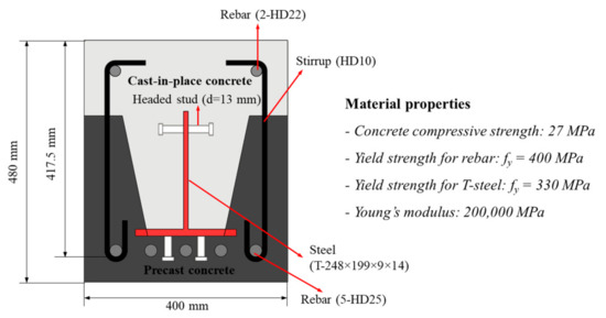
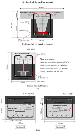
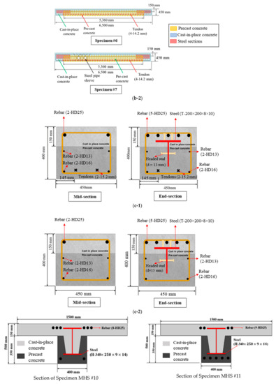
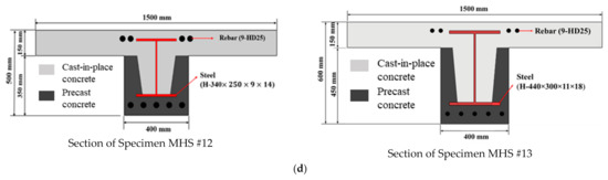
Figure 1.
Specimen details. (a) Cantilever Specimens #1, #2, and #3 (non-pre-stressed, CS1, CS2, and CP) [24]. (b-1) Specimens #4, #5 (pre-stressed); cross-sections of the test specimens with pinned joints [21,22]. (b-2) Specimens #6, #7 (pre-stressed); side views of the test specimens with pinned joints [21,22]. (c-1) Specimen #8 (pre-stressed); end and mid-section of a pre-stressed composite beam with fixed ends [7]. (c-2) Specimen #9 (non-pre-stressed); end and mid-section of a non-pre-stressed composite beam with fixed ends [7]. (d) Specimens #10 to #13; Steel-concrete composite beams with fixed ends (yield strength of concrete: 27 MPa, yield strength of rebar: 400 MPa; yield strength of steel: 240 MPa) [5].
Table 2.
Material properties of specimens for estimation of post-yield deflection [5,7,21,22,23,24,25,26].
2.2. Material Properties
Table 2 [5,7,21,22,23,24,25,26] presents material properties of Specimens #1 to #3 [24] and of Specimens #4 to #7 [21,22,25,26]. For Specimens #4 to #7, the cross-sections of the composite beams were reinforced with a 4-D25 mm top reinforcement, a 2-D25 mm bottom reinforcement, a 2-D13 mm reinforcement in the middle, and a D10 mm dowel bar. The compressive strength of the concrete (f’c) was 38.8 MPa, and the yield stress (fy) of the top and bottom reinforcement was 548.9 MPa. The yield stress (fy) of the D13 mm bar and dowel bar was 400 MPa. Tension bars were used for reinforcement in the middle prior to the placement of the concrete for the slab. A 2026.8 mm2 area of top steel reinforcement was placed at the ends, while four pre-stressed strands were installed at mid-span with a smaller steel area (1013.4 mm2), as shown in Figure 1b [21,22,25,26]. Four pieces of rebars with 25 mm diameter were used at each end to prevent unexpected support degradation during loading. Steel sections with a length of 970 mm were installed only at the ends. Four pre-stressing strands with diameter of 15.2 mm were installed 60.75 mm from the lower face of the specimens to provide additional flexural strength. Two steel pipe sleeve openings with diameter of 125 mm were located 1,200 mm and 1,650 mm from the center, as shown in Figure 1b. Diagonal reinforcements of D13 were installed to reinforce the opening loss. Figure 1c and Table 2 shows cross-sections of the fixed-end composite beams with (Specimen #8) and without (Specimen #9) pre-stressing forces. Two 15.2-mm-diameter pre-stressing tendons were introduced. In addition, 500 mm × 500 mm columns were installed 5 m apart to provide fixed conditions for Specimens #8 and #9. A column post with considerable reinforcements was placed to provide fixed-end conditions to the specimens during testing. A laboratory test was performed on Specimens #1 to #3 and #4 to #7 to determine the material properties. Coupon test results for Specimens #8 to #9 were also conducted. The compressive strength of the concrete (f’c) was 38.8 MPa, and the yield stress (fy) of the top and bottom reinforcements was 548.9 MPa. The yield stress (fy) of the D13 mm bar and dowel bar was 400 MPa for Specimens #4 to #9. The designed compressive strength of the concrete was 35 MPa.
3. Analytical Prediction of Post-Yield Deflection
3.1. Stiffness at Yield Limit State
In Figure 2 proposed by [28], the post-yield hysteretic structural behavior was estimated using the stiffness degradation in terms of normalized effective stiffness, which was calculated by dividing the effective stiffness of the hysteretic cycles by the stiffness at the yield limit state. The drift was also normalized by dividing the deflection of the hysteretic cycles by the deflection at the yield limit [28]. A quadratic equation was derived for the location of the neutral axis (c) relative to the top of Specimen MHS #10 after iteration, given by Equation (1) [23]. Force at the first yield state shown in Figure 3 was then estimated using Equation (2). Equation (4) was used to calculate deflection. The location of the neutral axis relative to the top of the beam was found to be 128.3 mm. Using the location of the neutral axis (c) and Equation (2), the moment of the Specimen MHS #10 at yield limit state was calculated to be 760.8 kN-m [23].
where,
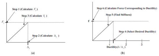
Figure 2.
Estimation of post-yield deflection based on stiffness degradation [28]: (a) stiffness at the yield limit state, (b) stiffness degradation.
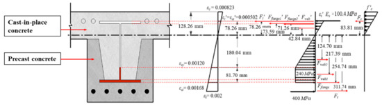
Figure 3.
Strain and stress (εc = 0.000823) at the yield limit state for Specimen #10 [23].
Symbols used in Equations (1) and (2) are explained as follow: : Stress factor, : concrete compresssive strength, b: beam width, c: depth of concrete compressive zone, d: beam effective depth, : area of rebar in compression, : area of rebar in tension, : yield stress of rebar, : yield stress of steel, : area of steel web, ; area of steel flange, : yield strain of steel, : concrete strain of 0.003, : centroid factor, : distance from tensile rebar to tensile flange, : distance from extreme compressive layer of concrete to compressive rebar, : distance from extreme compressive layer of concrete to compressive steel flange, : thickness of steel flange in compression, : thickness of steel flange in tension, : thickness of steel web in tension, : width of steel flange, y: yield, ny: not yield, p: plastic, and : Young’s modulus of steel.
The deflection was calculated based on the curvature–strain relationship of the beam section at the first yield of the rebar, as given by Equations (4) and (5) for fixed-end beams and cantilevers, respectively. The curvature (ϕy = M/EI= εy/(d − c)) can be used to calculate deflections.
The stiffness at the first yield of the rebar was eventually calculated based on force and deflection at yield limit state. In Figure 4d, forces and deflections at yields limit state are calculated for the Specimens #8 and #9 based on strain-compatibility, which were implemented to calculate stiffness at yields limit state.
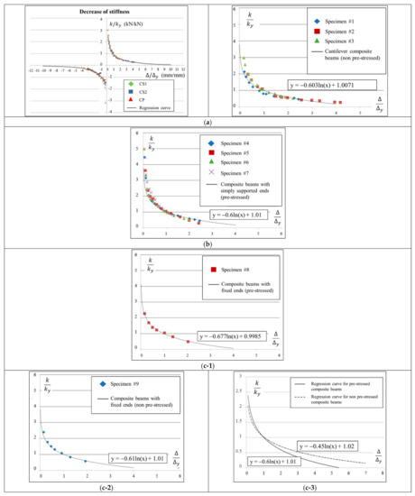
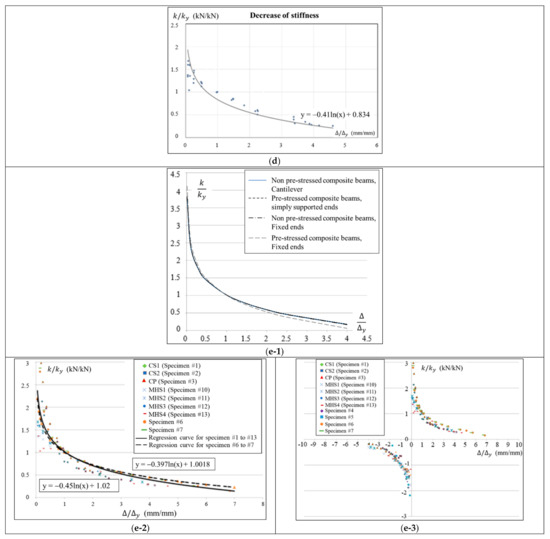
Figure 4.
Stiffness degradation tendencies (Specimens #1 to #13). (a) Non-pre-stressed cantilever beams (Specimens #1 to #3) for both loading directions [7,26]. (b) pre-stressed simply supported beams. (Specimens #4 to #7) [7]. (c-1) pre-stressed fixed-end beams (Specimens #8) [7]. (c-2) non-pre-stressed fixed-end beams (Specimens #9) [7]. (c-3) non-pre-stressed fixed-end beams (Specimens #8 and #9). (d) non-pre-stressed composite beams (Specimens #10 to #13) [5]. (e-1) Specimens #1 to #9 [7]. (e-2) All specimens (#1 to #13) vs. Specimens #6 and #7 [25]. (e-3) all specimens [25].
3.2. Stiffness Degradation
Stiffness degradation tendencies of all composite beam specimens are illustrated in Figure 4a–d. Regression analysis was performed to derive an equation representing degradation tendency. Regression results for all specimens are shown in Figure 4. The stiffness of the fixed end precast beams that were pre-stressed degraded more rapidly than those that were not pre-stressed, as shown in Figure 4c-3. It was observed that the post-yield deflection increased rapidly when pre-tensioned forces started to decrease, resulting in more rapid stiffness degradation in the pre-stressed section than in the non-pre-stressed section. In Figure 4e-3, degradation tendencies for the post-yield behavior of the precast composite beams are clearly shown based on normalized stiffness and deflection. Table 3 summarizes the regression results for Specimens #1 to #13.
Table 3.
Summary of stiffness degradation [7]
3.3. Prediction of Post-Yield Behavior
The loads (Fy, My) at the first yield of the rebar were calculated by iterating neutral axes and the corresponding concrete strain until equilibrium was found [23]. Table 4 [23] presents the post-yield behavior of pre-stressed Composite beam #8 with fixed-end, and Figure 5 compares the analytically calculated and experimental post-yield deflections. The post-yield load-displacement relationships for the composite beams were predicted using the following six-step procedure described below and in Figure 2, which was introduced in the authors’ previous studies [5,28].
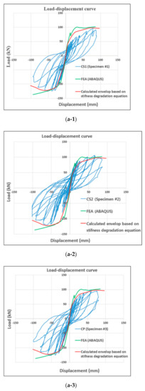
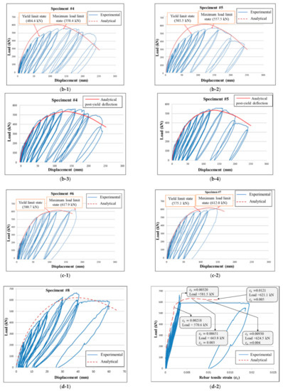
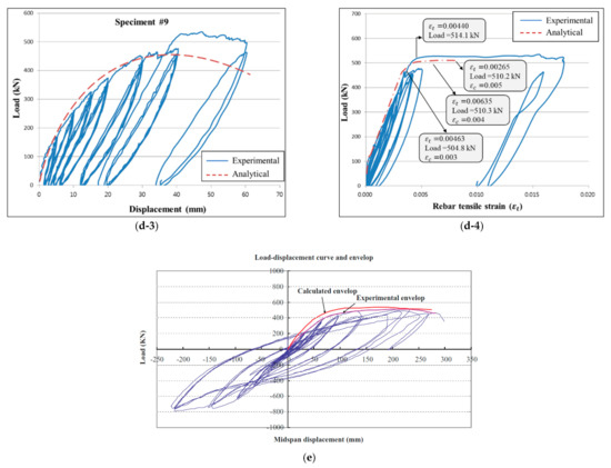
Figure 5.
Analytically calculated post-yield deflections vs. experimental post-yield deflections. (a) Post-yield deflection of pre-stressed Specimens #1 to #3, calculated using the degradation equation from Table 3 and Figure 4a (Specimens #1 to #3 compared with finite element analysis) [25,29]: (a-1) Specimen #1, (a-2) Specimen #2, (a-3) Specimen #3. (b-1) Specimen #4 (with no sleeve openings), Table 3, Figure 4b [25]. (b-2) Specimen #4 (with no sleeve openings), Table 3, Figure 4b [25]. (b) Post-yield deflection of pre-stressed Specimens #4 to #5, calculated using the degradation equation for simply supported beams from Figure 4b,e-2. (b-3) Specimen #4 (with no sleeve openings), Figure 4e-2 [24]; (b-4) Specimen #5 (with no sleeve openings), Figure 4e-2 [24]. (c) Post-yield deflection of pre-stressed Specimens #6 to #7, calculated using the degradation equation for simply supported beams from Figure 4b. (c-1) Specimen #6 (with sleeve openings), Table 3, Figure 4b [22]; (c-2) Specimens #7 (with sleeve openings), Table 3, Figure 4b [22]. (d) Post-yield deflection of Specimens #8 and #9. (d-1) Specimen #8, based on the degradation equation of Table 3, Figure 4c-1 [7]. (d-2) Load-strain relationship for Specimen #8 [7]. (d-3) Specimen #9, based on the degradation equation of Table 3, Figure 4c-2 [7]. (d-4) Load-strain relationship for Specimen #9 [7]. (e) Post-yield deflection of pre-stressed Specimens #10 using the degradation tendency of non-pre-stressed beams from Table 3 and Figure 4d [5].
- Calculate the load () on the composite beams at the yield limit, as shown in Figure 2 [23].
- Calculate the displacement () from Equations (4) and (5).
- Calculate the stiffness of the composite beams at the yield limit state from Figure 2a.
- Select the desired ductility from the load-displacement curve ( from Figure 2b.
- Find corresponding to the selected ductility from Figure 2b.
- Calculate and from Figure 2b in order to determine .
Forces at the yield load limit state were calculated using the strain compatibility-based approach. Deflections of 57.8 mm and 61.5 mm at the yield load limit state were calculated elastically for Specimens #4, 5 and #6, 7, respectively. Table 4 [23] describes the overall procedure for calculating the post-yield load-displacement relationship of precast composite beams. The first three columns in Table 4 [23] show the calculated values for load (Fy), deflection at the yield limit state (Δy), and stiffness (ky). The stiffness degradation tendency, obtained by normalizing the effective stiffness of the specimens with respect to the stiffness at first yield of the rebar, is presented in Figure 4. The stiffness degradation regression for non-pre-stressed cantilever beams (Specimens #1 to #3), shown as in Table 3, was used to obtain the post-yield load-displacement relationship for both positive and negative directions, as shown in Figure 5a-1–a3. In Table 4, a ductility between 1 and 5 was selected from the load-displacement curve shown in Figure 4. The post-yield deflection of pre-stressed Specimens #4, #5 and #6, #7 (Figure 5b-1,b-2,c-1,c-2) was calculated based on the stiffness degradation, , provided in Table 3 and Figure 4b. The post-yield deflection of pre-stressed Specimens #8 and #9 (Figure 5d-1,d-3) based on the stiffness degradation regressions, , found in Table 3 and Figure 4c-1,c-2, respectively. Figure 5e provide the post-yield deflection of Specimen #10 based on the stiffness degradation regression, shown in Figure 4d. A ductility between 1 and 5 was selected from the load-displacement curve. It was interesting to note that the post-yield deflection of pre-stressed Specimens #4 and #5, shown in Figure 5b-3,b-4, matched the test data better when it was calculated based on the global stiffness degradation tendency provided in Figure 4e-2, , which represented the stiffness degradation tendency of the thirteen specimens. The post-yield load-displacement relationships based on degradation tendencies (refer to Figure 4) were relatively well correlated with the test data, as shown in Figure 5. However, the use of an inappropriate beam degradation tendency can cause mismatches between test data and estimation. It should be noted that more consistent prediction of the post-yield load-displacement relationships for precast composite beams with various boundary conditions is possible when the predictions are based on big strength degradation data.
3.4. Verification Based on Finite Element Analysis
In Figure 6 [29], full-scale specimens (#1 to #3) [24] were modeled using a nonlinear finite element package to verify the proposed procedure predicting the post-yield behavior of the precast composite beams. Modeling techniques introduced in this study included symmetrical modeling, choice of elements, and modeling of embedded elements.
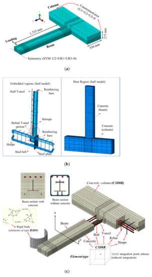
Figure 6.
Numerical model for Specimens #1 to #3 (CS1, CS2, and CP) [24,29]. (a) Symmetrical model with boundary conditions. (b) Mesh and element types. (c) Modeling of embedded elements.
3.4.1. Symmetrical Modeling
The important feature of symmetrical modeling is that it provides accurate results because the system of equations becomes much smaller, and computational errors are significantly reduced. The boundary conditions at the plane of symmetry were defined based on two general rules summarized by [30]. These two rules constrain both (1) translational displacement components normal to the plane of symmetry and (2) rotational displacement components with respect to the axis parallel to the plane of symmetry [31].
3.4.2. Choice of Elements
In this study, elements of type C3D8R and R3D4 were selected from the ABAQUS library [31] to predict the structural behavior of the tested specimens (CS1, CS2, and CP) [24]. C3D8R elements are three-dimensional elements known as reduced integration elements. These elements were preferred because they reduce the running time due to the fact that the integration was performed on a single integration point, as illustrated in Figure 6b. C3D8R elements were also suitable for nonlinear static analysis. Additionally, elements of type R3D4 were used to model a rigid body, as illustrated in Figure 6b. The rigid body employed in this study located a reference point at which a lateral displacement was applied.
3.4.3. Modeling of Embedded Elements
Modeling of embedded elements was carried out by assigning “embedded” and “host” elements. The embedded elements, which were embedded in the host elements, included T-steel, rebar, bolts, headed studs, stirrups, and hoops. ABAQUS checks the nodes of the embedded elements and host elements in a way that restrains the possible translational degrees of freedom of the embedded elements. Thus, a perfect bond between the embedded and host elements is fully achieved. The material properties of the embedded and host elements were obtained from test samples during testing of the full-scale specimens (CS1, CS2, and CP) [24]. The material properties used in the FE models are summarized in Table 5 [24,31]. The accuracy of the method predicting post-yield load-displacement relationships based on stiffness degradation proposed in this study was verified by non-linear finite element analysis, as shown in Figure 5a-1–a-3.
Table 5.
Material properties used in finite element analysis (Specimens #1 to #3 by [28]).
4. Results, Discussion and Conclusions
4.1. Contribution to the Understanding of the Post-Yield Structural Behavior of Pre-Stressed Precast Composite Beams Based on Proposed Degradation Equations
The post-yield structural behavior of pre-stressed precast composite beams was derived based on stiffness degradation, which reflected the hysteretic structural behavior obtained from test data collected from extensive experiments that included pre-stressed beams with both fixed and pinned boundary conditions. The regression results (Table 3) for stiffness degradation based on the effective stiffness and drift normalized by the stiffness and drift at the yield limit state were clustered for all 13 specimens with fixed and simply-supported ends. Equations derived separately with the presence of pre-stressing forces were also used to correlate and match the test data. The flexural moment capacity and post-yield deflection of the beams were more influenced by the bottom rebar in pre-stressed Specimen #8 than in non-pre-stressed Specimen #9, with strains of about 0.02 and 0.017 in the mid-section, respectively, demonstrating that lower ductility by 28% with pre-stressing forces was observed between the ductility of 5.3 and that 6.9 with non pre-stressed beams, as shown in Figure 4c-3. The stiffness degradation of both pre-stressed and non pre-stressed beams shows similar trends until a ductility of 1.0, as shown in Figure 4c-3. However, from a ductility of 1.0, a stiffness of fixed-end precast beams with pre-stressing degraded rapidly compared to those of beams that were not pre-stressed. Specifically, a stiffness degradation of pre-stressed beams decreased from 1.0 to 0.35, while that of non pre-stressed beams dropped 1.0 to 0.5 for the ductility range between 1.0 to 3.0.
4.2. Validated by Numerical Investigation
The post yield load-displacement relationships for steel-concrete composite beams in both positive and negative directions were verified numerically using nonlinear finite element analysis based on damaged concrete plasticity, showing that the complicated post-yield deflections related to ductility can be conveniently calculated using a simplified stiffness degradation tendency.
4.3. Further Refinement of the Degradation Model; The Applicability and Limitations of the Proposed Equations
The post-yield load-displacement relationships of precast composite beams with various boundary conditions were predicted with equations to predict the ultimate load limit of composite beams and their corresponding post-yield deflections. However, significantly different and inaccurate post-yield structural behavior was observed when an inappropriate beam degradation tendency was used. More degradation data for the effective stiffness under various boundary conditions need to be collected in order to increase the applicability of this prediction.
Author Contributions
Conceived and designed the experiments: W.-K.H.; performed the experiments: W.-K.H. and G.-T.L.; analyzed the experimental data: W.-K.H. and G.-T.L.; writing—original draft preparation: W.-K.H. and G.-T.L. All authors have read and agreed to the published version of the manuscript.
Funding
This research was supported by the Ministry of Education (NRF-2016R1D1A1A02937558) and the National Research Foundation of Korea (NRF) grant funded by the Korea government (MSIT) (No. 2019R1A2C2004965).
Institutional Review Board Statement
Not applicable.
Informed Consent Statement
Not applicable.
Acknowledgments
The above financial support is greatly appreciated.
Conflicts of Interest
The authors have no conflicts of interest to declare.
References
- Yang, Y.; Xue, Y.; Yu, Y.; Ma, N.; Shao, Y. Experimental study on flexural performance of partially precast steel reinforced concrete beams. J. Constr. Steel Res. 2017, 133, 192–201. [Google Scholar] [CrossRef]
- Nie, J.; Fan, J.; Cai, C.S. Stiffness and deflection of steel-concrete composite beams under negative bending. J. Struct. Eng. 2004, 130, 1842–1851. [Google Scholar] [CrossRef]
- Uy, B.; Bradford, M.A. Ductility of profiled composite beams. Part I: Experimental study. J. Struct. Eng. 1995, 121, 876–882. [Google Scholar] [CrossRef]
- Hajjar, J.F. Composite steel and concrete structural systems for seismic engineering. J. Constr. Steel Res. 2002, 58, 703–723. [Google Scholar] [CrossRef]
- Hong, W.K.; Kim, J.M.; Park, S.C.; Kim, S.I.; Lee, S.G.; Lee, H.C.; Yoon, K.J. Composite beam composed of steel and pre-cast concrete (modularized hybrid system, MHS) Part II: Analytical investigation. Struct. Des. Tall Spec. Build. 2009, 18, 891–905. [Google Scholar] [CrossRef]
- Faella, C.; Martinelli, E.; Nigro, E. Shear connection nonlinearity and deflections of steel-concrete composite beams: A simplified method. J. Struct. Eng. 2003, 129, 12–20. [Google Scholar] [CrossRef]
- Lim, G.T. An Investigation of Hybrid Pre-Stressed Composite Beam Flexural Capacity and Tendon Loss. Master’s Thesis, Kyung Hee University, Seoul, Korea, 2013. [Google Scholar]
- Nie, J.; Cai, C.S.; Wang, T. Stiffness and capacity of steel-concrete composite beams with profiled sheeting. Eng. Struct. 2005, 27, 1074–1085. [Google Scholar] [CrossRef]
- Nie, J.G.; Cai, C.S.; Wu, H.; Fan, J.S. Experimental and theoretical study of steel-concrete composite beams with openings in concrete flange. Eng. Struct. 2006, 28, 992–1000. [Google Scholar] [CrossRef]
- Wang, C.; Shen, Y.; Yang, R.; Wen, Z. Ductility and Ultimate Capacity of Prestressed Steel Reinforced Concrete Beams. Math. Probl. Eng. 2017, 2017, 1467940. [Google Scholar] [CrossRef]
- Nie, J.G.; Tian, C.Y.; Cai, C.S. Effective width of steel-concrete composite beam at ultimate strength state. Eng. Struct. 2008, 30, 1396–1407. [Google Scholar] [CrossRef]
- Liu, X.; Bradford, M.A.; Ataei, A. Flexural performance of innovative sustainable composite steel-concrete beams. Eng. Struct. 2017, 130, 282–296. [Google Scholar] [CrossRef]
- Liu, Y.; Guo, L.; Qu, B.; Zhang, S. Experimental investigation on the flexural behavior of steel-concrete composite beams with U-shaped steel girders and angle connectors. Eng. Struct. 2017, 131, 492–502. [Google Scholar] [CrossRef]
- Elamary, A.; Ahmed, M.M.; Mohmoud, A.M. Flexural behaviour and capacity of reinforced concrete-steel composite beams with corrugated web and top steel flange. Eng. Struct. 2017, 135, 136–148. [Google Scholar] [CrossRef]
- Chen, S. Experimental study of prestressed steel-concrete composite beams with external tendons for negative moments. J. Constr. Steel Res. 2005, 61, 1613–1630. [Google Scholar] [CrossRef]
- Saadatmanesh, H.; Albrecht, P.; Ayyub, B.M. Experimental study of prestressed composite beams. J. Struct. Eng. 1989, 115, 2348–2363. [Google Scholar] [CrossRef]
- Chen, S.; Gu, P. Load carrying capacity of composite beams prestressed with external tendons under positive moment. J. Constr. Steel Res. 2005, 61, 515–530. [Google Scholar] [CrossRef]
- Ayyub, B.M.; Sohn, Y.G.; Saadatamanesh, H. Prestressed composite girders I: Experimental study for negative moment. J. Struct. Eng. 1992, 118, 2743–2762. [Google Scholar] [CrossRef]
- Galvez, J.C.; Benitez, J.M.; Tork, B.; Casati, M.J.; Cendon, D.A. Splitting failure of precast prestressed concrete during the release of the prestressing force. Eng. Fail. Anal. 2009, 16, 2618–2634. [Google Scholar] [CrossRef]
- Ghallab, A. Calculating ultimate tendon stress in externally prestressed continuous concrete beams using simplified formulas. Eng. Struct. 2013, 46, 417–430. [Google Scholar] [CrossRef]
- Yoon, T.H. An Analytical and Experimental Investigation of Flexural Capacity for Steel-Pre-Stressed Composite Beam during Construction Phase. Master’s Thesis, Kyung Hee University, Seoul, Korea, 2011. [Google Scholar]
- Jeong, S.Y. Experimental and Analytical Investigation of Pre-Stressed Composite Beam Having Sleeves for Steel Pipes. Master’s Thesis, Kyung Hee University, Seoul, Korea, 2012. [Google Scholar]
- Hong, W.K.; Lee, Y.; Kim, S.; Kim, S.I.; Yun, Y.J. Analytical investigation of hybrid composite precast beams with modified strain compatibility for entire history of nominal flexural capacity. Struct. Des. Tall. Spec. Build. 2015, 24, 835–852. [Google Scholar] [CrossRef]
- Hong, W.K.; Jeong, S.Y.; Park, S.C.; Kim, J.T. Experimental investigation of an energy-efficient hybrid composite beam during the construction phase. Energy Build. 2012, 46, 37–47. [Google Scholar] [CrossRef]
- Yoon, D.Y. An Analytical and Experimental Investigation of Deflection for Steel Pre-Stressed Composite Beam during Construction Phase. Master’s Thesis, Kyung Hee University, Seoul, Korea, 2011. [Google Scholar]
- Park, S.C. Study of Steel-Reinforced Concrete Composite Beam Based on Strain Compatibility. Ph.D. Thesis, Kyung Hee University, Seoul, Korea, 2010. [Google Scholar]
- Kim, J.; Hong, W.K.; Lim, G.T. Losses of prestressed forces of pre-tensioned precast composite beams. Spec. Des. Tall Spec. Build. 2017, 26, e1339. [Google Scholar] [CrossRef]
- Hong, W.K. Development of Analytical Models for Reinforced Concrete Masonry Flexural Walls. Ph.D. Thesis, University of California, Los Angeles, CA, USA, 1989. [Google Scholar]
- Nzabonimpa, J.D.; Hong, W.K.; Kim, J. Strength and post-yield behavior of T section steel encased by structural concrete. Spec. Des. Tall Spec. Build. 2018, 27, e1447. [Google Scholar] [CrossRef]
- Liu, G.R.; Quek, S.S. Finite Element Method: A Practical Course, 1st ed.; Butterworth-Heinemann: Oxford, UK, 2003. [Google Scholar]
- Systemes, D. Abaqus Analysis User’s Guide; Dassault Systemes: Waltham, MA, USA, 2015; Volume 6.14-2. [Google Scholar]


Publisher’s Note: MDPI stays neutral with regard to jurisdictional claims in published maps and institutional affiliations. |
© 2021 by the authors. Licensee MDPI, Basel, Switzerland. This article is an open access article distributed under the terms and conditions of the Creative Commons Attribution (CC BY) license (https://creativecommons.org/licenses/by/4.0/).