2.1. Continuous Flow Problem
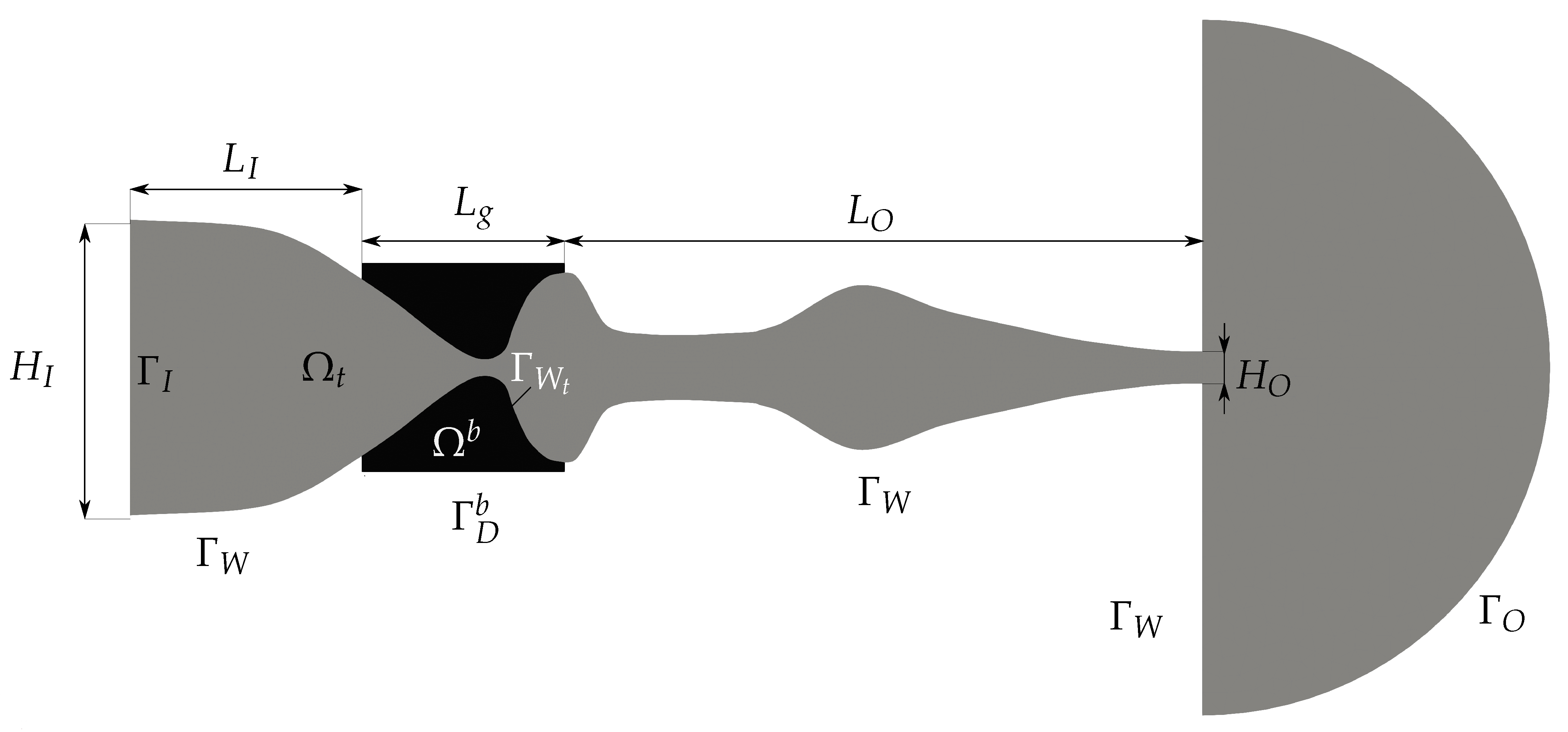
We consider compressible flow in a bounded domain for The boundary of consists of four disjointed parts: where represents the inlet, is the outlet and boundaries and denote impermeable fixed and moving walls, respectively.
The time dependence of the domain
is taken into account by using a regular one-to-one ALE mapping of the reference domain
onto the current configuration
. Next, we define the domain velocity
,
and the ALE derivative of the vector function
, where
and
:
, where
. Then the continuity equation, the N-S equations and the energy equation can be written in the ALE form
where
,
,
,
,
.
We have
, where
are
matrices depending on
w, and
with
, see [
11].
We use the following notation: p—pressure, —fluid density, E—total energy, —velocity vector, —absolute temperature, —specific heat at constant volume, —Poisson adiabatic constant, —dynamic viscosity, —second viscosity coefficients, —heat conduction coefficient, —components of the viscous part of the stress tensor.
Equation (
1) is completed by the following thermodynamical relations for pressure and absolute temperature
and equipped with initial and boundary conditions
with prescribed data
is the velocity of a moving wall and
denotes the unit outer normal.
2.2. Discrete Flow Problem
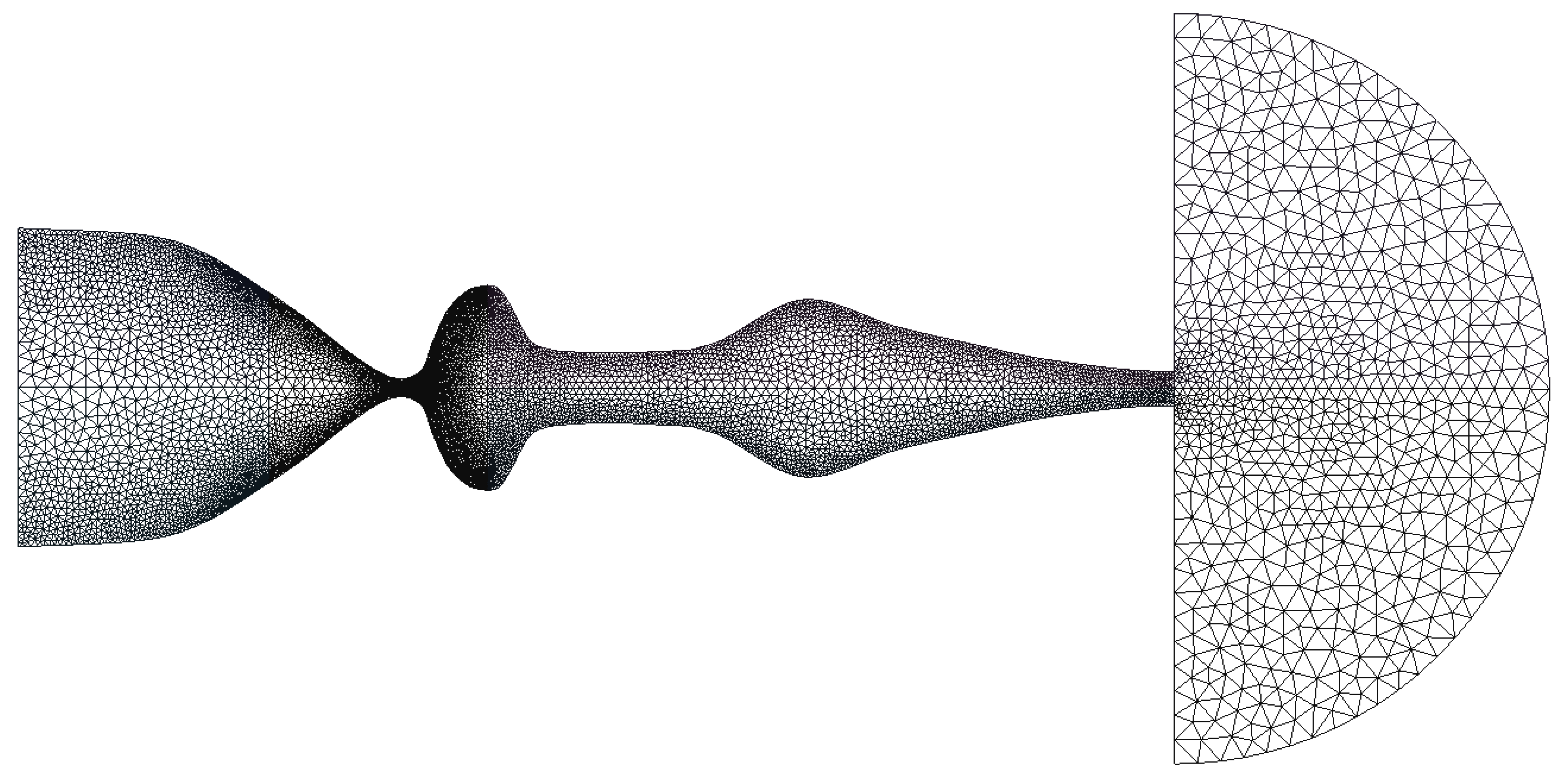
We describe the discretization, which is used in our in-house solver. We assume that
is a polygonal domain for every
. We denote by
a partition of the closure
into a finite number of closed triangles with disjoint interiors satisfying standard properties (see [
29]). We suppose that
is an image of
under the regular mapping
. Moreover, we assume that the ALE mapping
is continuous and affine in
.
By , we denote the system of all faces of all elements . Moreover, we introduce the sets of boundary faces “Dirichlet” boundary faces a Dirichlet condition is prescribed on and inner faces . Each is associated with a unit normal vector to . For , the normal has the same orientation as the outer normal to . For denotes the average of K and denotes the length of .
For each , there exist two neighboring elements such that . We use the convention that lies in the direction of , and lies in the opposite direction to . If , then the element adjacent to will be denoted by .
Now we introduce the space of piecewise polynomial functions
with
where
is an integer and
denotes the space of all polynomials on
K of degree
. It is possible to see that
. A function
is, in general, discontinuous on interfaces
. If
is a function defined on
, then by
and
, we denote the values of
on
considered from the interior of
and
respectively, (if these values make sense) and set
.
Thanks to properties of the expressions in the N-S equations, similarly as in [
11], the following forms are derived:
We set
,
or
and get the so-called symmetric (SIPG), incomplete (IIPG) or nonsymmetric (NIPG) version, respectively, of the discretization of viscous terms. In (
7) and (
8),
denotes a positive sufficiently large constant and
is the transposed matrix to
.
In the form (
9), symbols
and
denote the “positive” and “negative” parts of the matrix
defined in the following way. By [
30], this matrix is diagonalizable. It means that there exists a nonsingular matrix
such that
where
are eigenvalues of the matrix
. Now we define the “positive” and “negative” parts of the matrix
by
where
.
The boundary state
is defined on the basis of the Dirichlet boundary conditions (
3) and extrapolation:
In order to avoid spurious oscillations in the approximate solution in the vicinity of discontinuities or steep gradients, we apply artificial viscosity forms. They are based on the discontinuity indicator
By
, we denote the jump of the function
on the boundary
, and
denotes the area of the element
K. Then, we define the discrete discontinuity indicator
, and the artificial viscosity forms (see [
31])
with parameters
.
Because of the time discretization, we consider a partition
of the time interval
and denote
for
. We define the space
, where
with integers
. Here,
denotes the space of all polynomials in
t on
of degree
and the space
is defined in (
4). For
, we introduce the following notation:
In order to bind the solution on intervals
and
, we augment the resulting identity by the penalty expression
. The initial state
is defined as the
-projection of
on
, i.e.,
Furthermore, we define the prolongation of on the interval .
In what follows, we introduce the notation
for functions
defined in a set
.
Now, the
space-time DG approximate solution is defined as a function
satisfying (
20) and the following relation for
:
Remark 1. In the derivation of the discrete problem, the approximate solution and the test functions are considered as elements of the space . In practical computations, integrals appearing in the definitions of the forms and and also the time integrals over are evaluated with the aid of quadrature formulas using values of the approximate solution at discrete points of intervals . Therefore, the space is finite-dimensional, and the discrete problem is equivalent with a finite algebraic system for every .


