The Effect of Principal Component Analysis Parameters on Solar-Induced Chlorophyll Fluorescence Signal Extraction

Abstract

Solar-induced chlorophyll fluorescence (SIF), one of the three main releasing pathways of vegetation-absorbed photosynthetic active radiation, has been proven as an effective monitoring implementation of leaf photosynthesis, canopy growth, and ecological diversity. There exist three categories of SIF retrieval methods, and the principal component analysis (PCA) retrieval method is obtrusively eye-catching due to its brief, data-driven characteristics. However, we still lack a lucid understanding of PCA’s parameter settings. In this study, we examined if principal component numbers and retrieval band regions could have effects on the accuracy of SIF inversion under two controlled experiments. The results revealed that the near-infrared region could remarkably boost SIF’s retrieval accuracy, whereas red and near-infrared bands caused anomalous values, which subverted a traditional view that more retrieval regions might provide more photosynthetic information. Furthermore, the results demonstrated that three principal components would benefit more in PCA-based SIF retrieval. These arguments further help elucidate the more in-depth influence of the parameters on the PCA retrieval method, which unveil the potential effects of different parameters and give a parameter-setting foundation for the PCA retrieval method, in addition to assisting retrieval achievements.

1. Introduction

Solar-induced chlorophyll fluorescence (SIF), stimulated by vegetation-absorbed sunlight, is one of the three primary sun-releasing paths, along with photosynthesis and non-photochemical quenching (NPQ) [1]. As an effective proxy of vegetation photosynthetic functions, SIF has been proven to be more efficiently related to the gross primary productivity (GPP) compared with traditional reflectance vegetation indexes [2]. To illustrate this, SIF signals cover the 650–800 nm spectra and have two emission peaks: red light bands (around 685 nm) and near-infrared bands (around 740 nm). The former is mainly stimulated during photosystem II (PSII), whereas the latter is emitted by both photosystem I (PSI) and PSII [3].

SIF, as signals emitted actively by vegetation themselves, can also be detected by remote-sensing sensors, like reflectance spectra. To illustrate this, SIF signal retrieval refers to inverting atmospheric transference through known solar irradiances and surface radiances, thus reconstructing biochemical actions at the foliage level, including photosynthesis, fluorescence emission, and reflectance. Among the present sensors, there are several satellites with the potential to be utilized for SIF extraction: the Greenhouse Gases Observing Satellite (GOSAT), Global Ozone Monitoring Experiment-2 (GOME-2), SCIAMACHY, TanSat, and Orbiting Carbon Observatory 2 (OCO-2) [2,4,5,6]. Furthermore, the European Space Agency’s Fluorescence Explorer (FLEX) project is on schedule, and with the development of hyperspectral technology, computer technology, and their further applications in remote sensing, researchers have obtained information on the field, airborne, and satellite platforms. Thus, SIF has been successfully retrieved from remote sensing data and utilized in the real world [2,7,8,9].

There exist three main application categories of SIF: exploring vegetation photosynthesis, detecting vegetation growth stress effects, and other innovative applications [3,10]. First, numerous studies have shown that SIF can be used as one of the indicators to directly measure photosynthesis [11,12,13,14], and it can also be used to investigate the presently ambiguous relationships between SIF and many other photosynthesis factors (shown in

Table 1. Main applications of SIF in studies.

Applications	Variables	References
Photosynthesis estimation	Absorbed photosynthetic active radiation	[17,18]
	Gross primary productivity	[15,16]
	Light use efficiency	[14,17,19]
	Seasonal dynamics	[17,20,21]
	Vegetation type	[22,23]
	Chlorophyll content	[24,25]
Stress detection	Water deficit or drought	[27]
	Nitrogen deficit	[26]
	Heat	[28]
Creative applications	Extreme accidents	[30,31,32]
	Temperature of canopy	[29]

). To be specific, significant progress has been made in unearthing the relationships between factors, such as the GPP [15,16], absorbed photosynthetic active radiation (APAR) [17,18], light use efficiency (LUE) [14,17,19], seasonal dynamics [17,20,21], vegetation type [22,23], and chlorophyll content [24,25]. Secondly, using SIF to reveal the stress effects of water, nitrogen, and other factors is also an important research field [26,27,28]. Furthermore, there are also some novel applications, such as canopy temperature detection [29], extreme events analysis [30,31,32], and so on. Those prosperous prospects promise a future for SIF applications.

At present, SIF retrieval methods fall into three categories: algorithms based on atmospheric radiative transmission, simplified physically based model algorithms, and data-driven algorithms [33]. Based on atmospheric radiation transmission and simulating the absorption and scattering of solar radiation, the atmospheric radiation transmission methods were established to simultaneously solve SIF signals. The Fraunhofer line discrimination (FLD) algorithms, spectral fitting method (SFM), and their derivative methods are representative examples. These algorithms have an excellent physical basis, whereas the disadvantage is that the accuracy could interfere with the exactitude of the solar radiation, input as parameters. Fortunately, the SFM algorithms have been adopted as the SIF inversion algorithm of the FLEX project [18]. There are also two families of algorithms: the simplified physically based model methods and the data-driven statistical approaches. The latter always involve some traditional statistical methods, like principal component analysis (PCA), or singular value decomposition (SVD) analysis. Through these classic tools, signals received by the sensors could be seen as the co-production of the non-fluorescent signals and fluorescent signals, thus constructing a training set of non-fluorescent spectra and extracting features. Using these features to represent non-fluorescent signals, thus escaping complex expressions of atmospheric situations and transmissions, data-driven algorithms seek to compromise between both physical models and simple experimental methods. The PCA retrieval algorithm considers whole radiance signals as the sum of non-fluorescence and fluorescence and then uses principal components (PCs) [34] to represent complex and hard-to-calculate variables. At the same time, facing massive data volumes, the PCA algorithm could eliminate redundant information and obtain vital features. Thus, the advantage of this method is that it avoids the complex calculation of radiation transmission and improves efficiency, while the disadvantage is that the parameter setting would affect the inversion results. However, there currently exists a lack of in-depth discussion on the parameter selection: the effect of different principal component numbers and band regions on the accuracy of SIF retrieval.

Thus, the main target of this research is to analyze the effect of the PC numbers and spectral band regions on the accuracy of SIF retrieval, especially in our study region. Then, PCA methods would benefit and provide a more reliable basis for PCA algorithm parameter settings in SIF retrieval.

2. Materials and Methods

2.1. Research Region

The research area, Danzhou City, located in Hainan Province, China, has abundant vegetation resources and thus is extremely valuable for SIF retrieval.

Table 2. An introduction of the study area and data.

	Hyperspectral Data
Study area	Danzhou, Hainan Province, China
Spatial resolution	1 m × 1 m
Spectral resolution	0.11 nm
Spectral band number	1004
Spectral regions	669.84 nm~780.32 nm
Acquiring time	25 May 2020
Data format	BIL
Data unit	Radiance (mW/cm2·str·um) × 1000.00

is a brief introduction of the experimental data. Since previous SIF retrievals and applications were mostly based on satellite data, the research area focused on the intercontinental and global scales [3], and since most of their performances were restricted by spatial and spectral resolutions, vegetation fluorescence in small scales and in small areas for monitoring and applications are thus demanding.

To illustrate this, the research area was covered by vegetation (mainly forest and cultivated fields) to a large extent, mainly in the northern and southeastern areas. There were a set of buildings and other human-made infrastructures that were situated in the middle and southwestern areas, showing extremely bright radiances in Figure 1.

2.2. Method

The data-driven PCA algorithm regards the radiance signals ($L_{TOA}$) as the sum of non-fluorescence and fluorescence as follows:

$$L_{TOA}=I_{sol}·\frac{{\mu }_0}{\pi }·\left[{\rho }_0+\frac{{\rho }_s·T_{\uparrow \downarrow }}{1-S·{\rho }_s}\right]+\frac{F_s·T_{\uparrow }}{1-S·{\rho }_s}$$

(1)

where $I_{sol}$ is the sun irradiance from the top of the atmosphere (TOA), ${\mu }_0$ is the cosine of the sun’s zenith angle, ${\rho }_0$ refers to the atmospheric backscattering, $S$ is the reflection from the hemisphere, ${\rho }_s$ is the surface reflectance, $T_{\uparrow }$ is the atmospheric upward transmittance, and $F_s$ is the fluorescence signals, which are our final demands. The first term on the right side in Equation (1) is the non-fluorescent spectra, and the second term is the fluorescent spectra.

The non-fluorescence can be decomposed into high-frequency signals (the absorption of Earth’s atmosphere through solar radiation’s descent) and low-frequency signals (including ${\rho }_0$, $S$, and ${\rho }_s$). The low-frequency signals can be characterized as a low-order polynomial function of the wavelength (λ), while the high-frequency term can be regarded as a linear formula of the non-fluorescent characteristics. Therefore, the PCA retrieval method was used to extract features from the training samples, which means that the first term of Equation (1) can be expressed as

$$I_{sol}·\frac{{\mu }_0}{\pi }·\left[{\rho }_0+\frac{{\rho }_s·T_{\uparrow \downarrow }}{1-S·{\rho }_s}\right]\approx I_{sol}·\frac{{\mu }_0}{\pi }·{\displaystyle \sum }_{i=0}^{n_p}\left({\alpha }_i·{\lambda }^i\right)·{\displaystyle \sum }_{j=1}^{n_{pc}}\left({\beta }_j·P{C}_j\right)$$

(2)

where $P{C}_j$ is the principal component vectors, ${\beta }_j$ is the coefficient of the principal component, $n_p$ is the order of the polynomial, and $n_{pc}$ is the number of PCs.

On the other hand, the fluorescence spectra could be composed of the $F_s$ fluorescence signals and the high-frequency signals in the atmospheric upstream. The latter can be further represented by PCs as well. Therefore, the second term in Equation (1) can be expressed as

$$\frac{F_s·T_{\uparrow }}{1-S·{\rho }_s}\approx F_s·exp\left[\ln \left({\displaystyle \sum }_{j=1}^{n_{pc}}\left({\beta }_j·P{C}_j\right)\right)\frac{\sec {\theta }_v}{\sec {\theta }_v+\sec {\theta }_0}\right]$$

(3)

where ${\theta }_v$ and ${\theta }_0$ are the view zenith angle and the solar zenith angle, respectively, and the upward atmospheric radiation is ignored in the calculations. At the same time, assuming that within the selected fitting window, fluorescence spectra obey the Gaussian distribution. Thus, Equation (3) can be simplified as

$$\frac{F_s·T_{\uparrow }}{1-S·{\rho }_s}\approx F_s·h_f$$

(4)

where $h_f$ is an SIF spectral function.

In summary, the final on-plane radiance on the fluorescent surface can be simplified as follows:

$$L_{TOA}\left(\mathsf{\alpha },\mathsf{\beta },F_s\right)=I_{sol}·\frac{{\mu }_0}{\pi }·{\displaystyle \sum }_{i=0}^{n_p}\left({\alpha }_i·{\lambda }^i\right)·{\displaystyle \sum }_{j=1}^{n_{pc}}\left({\beta }_j·P{C}_j\right)+F_s·h_f$$

(5)

where $h_f$ is as follows:

$${\mathrm{h}}_{\mathrm{F}}=\exp \left(\frac{-{\left(\mathsf{\lambda }-{\mathrm{u}}_{\mathrm{h}}\right)}^2}{2·{\mathsf{\sigma }}_{\mathrm{h}}^2}\right)$$

(6)

Therefore, this linear least squares problem paves the way for solving SIF signals. In this study, the steps of the PCA algorithm for parameter analysis are as follows:

(1)

Training sample selection: We first select red and near-infrared band regions to calculate the normalized difference vegetation index (NDVI). Then, this study uses 0.1 as the NDVI threshold to extract non-vegetation pixels in the whole image and extracts the corresponding radiance spectra as input samples for PCA.

(2)

Conduct two control variate experiments:

Since the band numbers could cause different results, in the first experiment, we set one, two, three, and four PCs and then analyze their influence toward the final SIF retrieval results.

On the other hand, there are two well-known Fraunhofer dark lines near the red band (around 687 nm) and near-infrared band (around 760 nm) that can be used for SIF inversion. In this way, the second part of the study uses the two regions to conduct a control variable experiment. Group A uses the radiance spectra at 680–690 nm and 750–780 nm for SIF inversion (referring to R-NIR inversion), whereas group B only uses the radiance spectra at 750–780 nm (referring to NIR inversion). The reason why only red band inversion is not applied is that, in the red band regions, SIF signals are severely affected by scattering and reabsorption in the vegetation canopy, which causes unignorable difficulties in retrieving SIF. Nevertheless, the near-infrared bands are more suitable and widely used for SIF inversion [35,36,37,38,39].

2.3. Evaluation

The current SIF verification methods include two main categories: site-measured data and existing SIF products. Since the experimental area was covered by dense forests, it was difficult to measure the variables directly. Furthermore, most current SIF datasets have limited temporal and spatial resolutions to meet the needs of accurate evaluation, and thus there remains the problem of obtaining instantaneous, high-resolution SIF maps [3]. Thus, to verify our results, the SFM algorithm was also used to retrieve SIF in this study.

The core of the SFM algorithm involves using broader spectral regions to fit the least squares formula and then obtaining the SIF and reflectance curves simultaneously. The least squares function is shown in Equation (7):

$$min{{\displaystyle \sum }}^{ }{\left(L_{TOC}\left(\mathsf{\lambda }\right)-\rho \left(\mathsf{\lambda }\right)L_{WLR}\left(\mathsf{\lambda }\right)-F_s\left(\mathsf{\lambda }\right)\right)}^2$$

(7)

where $\mathsf{\lambda }$ is the corresponding wavelength in the fitting windows, $L_{TOC}$ is the radiance signals, $L_{WLR}$ is the radiance of the standard plate, $\rho$ is the surface reflectance, and $F_s$ is the SIF signal function from the top of the canopy (TOC). The SIF and reflectance signal curves could be obtained by least squares fitting through the radiance and irradiance signals. In all, this research jointly compared and certificated the inversion results of the SFM and PCA algorithms.

3. Results

The inversion results of the PCA data-driven algorithm might have had some ambiguous relationships with the characteristics of different training samples, wavelength regions, and the number of PCs with simultaneously changing polynomial orders. Due to the restriction of the amount of our data volumes, we selected all pixels with NDVI values less than 0.1 as non-fluorescent signals. What is more, the PC numbers and the polynomial orders were changing together, and thus this study mainly aimed to elucidate the influence of the PC numbers and spectral band regions on the accuracy of the SIF inversion.

3.1. The Analysis of the Principal Component Numbers

In this study, 1–4 PCs were selected for the analysis of SIF retrieval, and the results are shown in Figure 2. According to Figure 2, the PCs were inevitably affecting the accuracy of SIF inversion. As the previous literature has illustrated, the global spatial SIF maps from OCO-2 products show that SIF values had a range from −4 $\mathsf{mW}{\mathsf{m}}^{-2}\mathsf{s}{\mathsf{r}}^{-1}\mathsf{n}{\mathsf{m}}^{-1}$ to 4 $\mathsf{mW}{\mathsf{m}}^{-2}\mathsf{s}{\mathsf{r}}^{-1}\mathsf{n}{\mathsf{m}}^{-1}$ [40]. Furthermore, when probing the moist tropical or subtropical forests, the researchers found out that even the lowest SIF value was larger than 0.2 $\mathsf{mW}{\mathsf{m}}^{-2}\mathsf{s}{\mathsf{r}}^{-1}\mathsf{n}{\mathsf{m}}^{-1}$ [32]. Thus, when inverted from one or two PCs, the SIF intensity values easily fell into invalidity, showing either too many negative values (Figure 2a) or extremely miniscule values (Figure 2b). Another obtrusive interference was that in this approach, as shown in Equation (5), the SIF values were derived partly by ${\lambda }^i$, which means that the SIF values were anomalously high when considering a higher polynomial order (magnitude of four or higher), which are illustrated in Figure 2d. Above all, three PCs would be apropos for PCA-based SIF retrieval. In comparison, the spectral band regions would have a greater and analytical influence on the results of SIF inversion.

3.2. The Analysis of the Spectral Band Regions

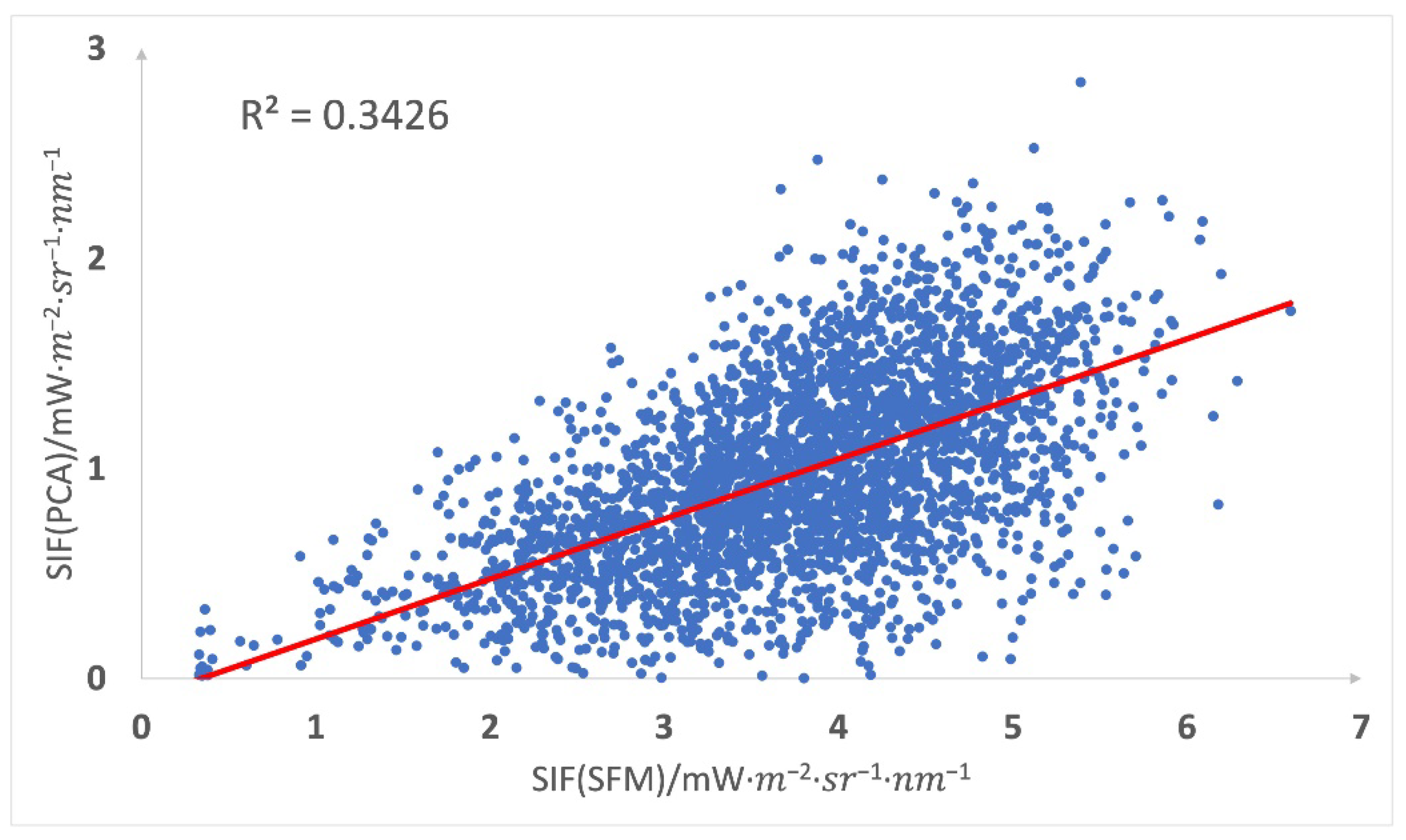
In this set of control experiments, we aimed at exploring the influence of the spectral band regions on SIF inversion. Thus, we first set the number of PCs to three when using the PCA and the polynomial as third order to ensure a normal SIF value range.

Figure 3 shows the data-driven algorithm inversion results of groups A and B. From a qualitative point of view, the SIF value distributions were both consistent with the surface radiance images (shown in Figure 1), and the SIF value results all showed obvious directional effects: the northern side of the picture showed significantly higher SIF values than the southern side. To illustrate this, the high vegetation area in the north determined the more significant SIF signals, whereas the texture of the lower SIF area in the middle and east revealed that these areas were covered by buildings or roads, where there was no vegetation emitting fluorescence at all. One main difference between Figure 3a,b is the square building structure in southwestern area, showing obtrusively high and relatively moderate values using R-NIR and sole NIR regions, respectively. Due to the rationality of SIF, all human-made structures do not emit chlorophyll fluorescence, which indicates that the values in Figure 3a are invalid, while the NIR bands are enough to retrieve SIF.

From a numerical point of view, the calculated SIF value ranges of group A and group B were 0–3.108 and 0–17.846 $\mathsf{mW}{\mathsf{m}}^{-2}\mathsf{s}{\mathsf{r}}^{-1}\mathsf{n}{\mathsf{m}}^{-1}$, respectively, within the normal range of SIF (0–20 $\mathsf{mW}{\mathsf{m}}^{-2}\mathsf{s}{\mathsf{r}}^{-1}\mathsf{n}{\mathsf{m}}^{-1}$), but there was an obvious difference in the magnitudes. In further comparing the SIF frequency distribution maps through Figure 4, the SIF value map obtained by using the R-NIR regions was concentrated around 0.7 $\mathsf{mW}{\mathsf{m}}^{-2}\mathsf{s}{\mathsf{r}}^{-1}\mathsf{n}{\mathsf{m}}^{-1}$, while the SIF values obtained by the NIR only region was focused around 5 $\mathsf{mW}{\mathsf{m}}^{-2}\mathsf{s}{\mathsf{r}}^{-1}\mathsf{n}{\mathsf{m}}^{-1}$. This indicates that R-NIR inversion is obviously less superior. Existing studies have shown that the near-infrared band can better retrieve SIF, since the influence of vegetation canopy scattering and reabsorption would be lower in this region [37]. The results of our experiment also confirm this position; that is, the NIR region retrieval is closer to the normal range of SIF values and also SFM verification, which will be stated in the following section.

3.3. Verification

To verify the retrieval results of our experiments, SFM algorithm inversion was used in this study. Figure 5 shows the results of the SFM algorithm and the corresponding SIF frequency distribution diagram in NIR, whereas Figure 6 shows the SIF correlation analysis of both the SFM and PCA algorithms.

In terms of numerical verification (as shown in Figure 5), the SIF values of the SFM algorithm fell around 4 $\mathsf{mW}{\mathsf{m}}^{-2}\mathsf{s}{\mathsf{r}}^{-1}\mathsf{n}{\mathsf{m}}^{-1}$, which was close to the NIR retrieval values in Figure 4. It is worth pointing out that the SFM approach combines both the characteristics of the physical model and the data-driven algorithm, leading to more reliable results. However, the calculation process used the same irradiance data, and thus errors might still accrete to some extent that cannot be ruled out.

Besides that, this study also randomly selected 3000 pixels in the image and performed a least squares fitting analysis of the corresponding SFM algorithm and PCA algorithm values. The diagram is shown in Figure 6. It is clear that the results had a certain correlation ($R^2$ = 0.3426), which proves that the SIF trends of the two algorithms were consistent, although the actual values in the corresponding pixels were different.

This research also raises three questions worthy of further discussion. First, the band regions can be further refined. In this study, through controlled band regions, NIR band inversion performed better than the results of R-NIR inversion by the comparison of SIF value distribution. However, the spatial resolution of the hyperspectral data was 1 nm, whereas the near-infrared band selected in the study covered 30 bands. Neighboring bands may still cause information redundancy. Therefore, more in-depth research on band selection needs to be further explored. Another question is how to improve the verification method, which is necessary. The verification method in this study can only be determined from a comparison perspective and not an exact measurement of SIF values. This also gives further difficulties for determining the band regions. Finally, after uncovering the PCA parameters’ influence toward the SIF retrieval results in this study, it is indispensable to confirm its transferability to a broader spatial and dataset extent.

4. Conclusions

The PCA data-driven algorithm takes advantage of PCA to eliminate data redundancy and represent complex atmospheric information in a succinct way thus simplifying the cumbersome retrieval process. In this study, two main parameters required in the implementation of the PCA retrieval algorithm—PC numbers and band regions—were analyzed, and the results of SFM algorithm inversion were utilized for cross-verification. The results demonstrated that three PCs could best illustrate information for SIF retrieval, and that the number of PCs severely interferes with the accuracy of SIF extraction, causing anomalously high values when encountering higher polynomial orders, and the NIR bands could boost the accuracy for fluorescence extraction better than the R-NIR regions. Thus, this study can provide a reference for the application of PCA algorithms in SIF retrieval. In addition, the reliability of PCA algorithms needs to be further researched by using more datasets in the future.

References

1. Pfündel, E. Estimating the contribution of photosystem I to total leaf chlorophyll fluorescence. Photosynth. Res. 1998, 56, 185–195. [Google Scholar] [CrossRef]
2. Frankenberg, C.; Butz, A.; Toon, G. Disentangling chlorophyll fluorescence from atmospheric scattering effects in O2 A-band spectra of reflected sun-light. Geophys. Res. Lett. 2011, 38. [Google Scholar] [CrossRef]
3. Mohammed, G.H.; Colombo, R.; Middleton, E.M.; Rascher, U.; van der Tol, C.; Nedbal, L.; Goulas, Y.; Pérez-Priego, O.; Damm, A.; Meroni, M. Remote sensing of solar-induced chlorophyll fluorescence (SIF) in vegetation: 50 years of progress. Remote Sens. Environ. 2019, 231, 111177. [Google Scholar] [CrossRef]
4. Du, S.; Liu, L.; Liu, X.; Zhang, X.; Zhang, X.; Bi, Y.; Zhang, L. Retrieval of global terrestrial solar-induced chlorophyll fluorescence from TanSat satellite. Sci. Bull. 2018, 63, 1502–1512. [Google Scholar] [CrossRef] [Green Version]
5. Joiner, J.; Guanter, L.; Lindstrot, R.; Voigt, M.; Vasilkov, A.; Middleton, E.; Huemmrich, K.; Yoshida, Y.; Frankenberg, C. Global monitoring of terrestrial chlorophyll fluorescence from moderate spectral resolution near-infrared satellite measurements: Methodology, simulations, and application to GOME-2. Atmos. Meas. Tech. 2013, 6, 2803–2823. [Google Scholar] [CrossRef] [Green Version]
6. Guanter, L.; Zhang, Y.; Jung, M.; Joiner, J.; Voigt, M.; Berry, J.A.; Frankenberg, C.; Huete, A.R.; Zarco-Tejada, P.; Lee, J.-E. Global and time-resolved monitoring of crop photosynthesis with chlorophyll fluorescence. Proc. Natl. Acad. Sci. USA 2014, 111, E1327–E1333. [Google Scholar] [CrossRef] [Green Version]
7. Moya, I.; Guyot, G.; Goulas, Y. Remotely sensed blue and red fluorescence emission for monitoring vegetation. ISPRS J. Photogramm. Remote Sens. 1992, 47, 205–231. [Google Scholar] [CrossRef]
8. Joiner, J.; Yoshida, Y.; Vasilkov, A.; Middleton, E. First observations of global and seasonal terrestrial chlorophyll fluorescence from space. Biogeosciences 2011, 8, 637–651. [Google Scholar] [CrossRef] [Green Version]
9. Köhler, P.; Guanter, L.; Joiner, J. A linear method for the retrieval of sun-induced chlorophyll fluorescence from GOME-2 and SCIAMACHY data. Atmos. Meas. Tech. 2015. [Google Scholar] [CrossRef] [Green Version]
10. Frankenberg, C.; Berry, J. Solar induced chlorophyll fluorescence: Origins, relation to photosynthesis and retrieval. In Reference Module in Earth Systems and Environmental Sciences; Elsevier: Amsterdam, The Netherlands, 2018. [Google Scholar]
11. Li, J.; Zhang, Y.; Gu, L.; Li, Z.; Li, J.; Zhang, Q.; Zhang, Z.; Song, L. Seasonal variations in the relationship between sun-induced chlorophyll fluorescence and photosynthetic capacity from the leaf to canopy level in a rice crop. J. Exp. Bot. 2020, 71, 7179–7197. [Google Scholar] [CrossRef]
12. Maguire, A.J.; Eitel, J.U.; Griffin, K.L.; Magney, T.S.; Long, R.A.; Vierling, L.A.; Schmiege, S.C.; Jennewein, J.S.; Weygint, W.A.; Boelman, N.T. On the Functional Relationship between Fluorescence and Photochemical Yields in Complex Evergreen Needleleaf Canopies. Geophys. Res. Lett. 2020, 47, e2020GL087858. [Google Scholar] [CrossRef]
13. Yang, J.; Yang, S.; Zhang, Y.; Shi, S.; Du, L. Improving characteristic band selection in leaf biochemical property estimation considering interrelations among biochemical parameters based on the PROSPECT-D model. Opt. Express 2021, 29, 400–414. [Google Scholar] [CrossRef] [PubMed]
14. Dechant, B.; Ryu, Y.; Badgley, G.; Zeng, Y.; Berry, J.A.; Zhang, Y.; Goulas, Y.; Li, Z.; Zhang, Q.; Kang, M. Canopy structure explains the relationship between photosynthesis and sun-induced chlorophyll fluorescence in crops. Remote Sens. Environ. 2020, 241, 111733. [Google Scholar] [CrossRef] [Green Version]
15. Perez-Priego, O.; Guan, J.; Rossini, M.; Fava, F.; Wutzler, T.; Moreno, G.; Carvalhais, N.; Carrara, A.; Kolle, O.; Julitta, T. Sun-induced chlorophyll fluorescence and photochemical reflectance index improve remote-sensing gross primary production estimates under varying nutrient availability in a typical Mediterranean savanna ecosystem. Biogeosciences 2015, 12, 6351–6367. [Google Scholar] [CrossRef] [Green Version]
16. Goulas, Y.; Fournier, A.; Daumard, F.; Champagne, S.; Ounis, A.; Marloie, O.; Moya, I. Gross primary production of a wheat canopy relates stronger to far red than to red solar-induced chlorophyll fluorescence. Remote Sens. 2017, 9, 97. [Google Scholar] [CrossRef] [Green Version]
17. Wieneke, S.; Burkart, A.; Cendrero-Mateo, M.; Julitta, T.; Rossini, M.; Schickling, A.; Schmidt, M.; Rascher, U. Linking photosynthesis and sun-induced fluorescence at sub-daily to seasonal scales. Remote Sens. Environ. 2018, 219, 247–258. [Google Scholar] [CrossRef]
18. De Grave, C.; Verrelst, J.; Morcillo-Pallarés, P.; Pipia, L.; Rivera-Caicedo, J.P.; Amin, E.; Belda, S.; Moreno, J. Quantifying vegetation biophysical variables from the Sentinel-3/FLEX tandem mission: Evaluation of the synergy of OLCI and FLORIS data sources. Remote Sens. Environ. 2020, 251, 112101. [Google Scholar] [CrossRef]
19. Cheng, Y.-B.; Middleton, E.M.; Zhang, Q.; Huemmrich, K.F.; Campbell, P.K.; Cook, B.D.; Kustas, W.P.; Daughtry, C.S. Integrating solar induced fluorescence and the photochemical reflectance index for estimating gross primary production in a cornfield. Remote Sens. 2013, 5, 6857–6879. [Google Scholar] [CrossRef] [Green Version]
20. Campbell, P.K.; Huemmrich, K.F.; Middleton, E.M.; Ward, L.A.; Julitta, T.; Daughtry, C.S.; Kustas, W.P. Diurnal and seasonal variations in chlorophyll fluorescence associated with photosynthesis at leaf and canopy scales. Remote Sens. 2019, 11, 488. [Google Scholar] [CrossRef] [Green Version]
21. Zhang, Y.; Commane, R.; Zhou, S.; Williams, A.P.; Gentine, P. Light limitation regulates the response of autumn terrestrial carbon uptake to warming. Nat. Clim. Chang. 2020, 10, 739–743. [Google Scholar] [CrossRef]
22. Damm, A.; Guanter, L.; Paul-Limoges, E.; Van der Tol, C.; Hueni, A.; Buchmann, N.; Eugster, W.; Ammann, C.; Schaepman, M.E. Far-red sun-induced chlorophyll fluorescence shows ecosystem-specific relationships to gross primary production: An assessment based on observational and modeling approaches. Remote Sens. Environ. 2015, 166, 91–105. [Google Scholar] [CrossRef]
23. Malenovský, Z.; Lucieer, A.; King, D.H.; Turnbull, J.D.; Robinson, S.A. Unmanned aircraft system advances health mapping of fragile polar vegetation. Methods Ecol. Evol. 2017, 8, 1842–1857. [Google Scholar] [CrossRef] [Green Version]
24. Pacheco-Labrador, J.; Perez-Priego, O.; El-Madany, T.S.; Julitta, T.; Rossini, M.; Guan, J.; Moreno, G.; Carvalhais, N.; Martín, M.P.; Gonzalez-Cascon, R. Multiple-constraint inversion of SCOPE. Evaluating the potential of GPP and SIF for the retrieval of plant functional traits. Remote Sens. Environ. 2019, 234, 111362. [Google Scholar] [CrossRef]
25. Camino, C.; Gonzalez-Dugo, V.; Hernandez, P.; Zarco-Tejada, P.J. Radiative transfer Vcmax estimation from hyperspectral imagery and SIF retrievals to assess photosynthetic performance in rainfed and irrigated plant phenotyping trials. Remote Sens. Environ. 2019, 231, 111186. [Google Scholar] [CrossRef]
26. Jia, M.; Colombo, R.; Rossini, M.; Celesti, M.; Zhu, J.; Cogliati, S.; Cheng, T.; Tian, Y.; Zhu, Y.; Cao, W. Estimation of leaf nitrogen content and photosynthetic nitrogen use efficiency in wheat using sun-induced chlorophyll fluorescence at the leaf and canopy scales. Eur. J. Agron. 2021, 122, 126192. [Google Scholar] [CrossRef]
27. Chen, A.; Mao, J.; Ricciuto, D.; Xiao, J.; Frankenberg, C.; Li, X.; Thornton, P.E.; Gu, L.; Knapp, A.K. Moisture availability mediates the relationship between terrestrial gross primary production and solar-induced chlorophyll fluorescence: Insights from global-scale variations. Glob. Chang. Biol. 2020. [Google Scholar] [CrossRef] [PubMed]
28. Song, L.; Guanter, L.; Guan, K.; You, L.; Huete, A.; Ju, W.; Zhang, Y. Satellite sun-induced chlorophyll fluorescence detects early response of winter wheat to heat stress in the Indian Indo-Gangetic Plains. Glob. Chang. Biol. 2018, 24, 4023–4037. [Google Scholar] [CrossRef] [Green Version]
29. Zarco-Tejada, P.J.; González-Dugo, V.; Berni, J.A. Fluorescence, temperature and narrow-band indices acquired from a UAV platform for water stress detection using a micro-hyperspectral imager and a thermal camera. Remote Sens. Environ. 2012, 117, 322–337. [Google Scholar] [CrossRef]
30. Wang, S.; Zhang, Y.; Ju, W.; Porcar-Castell, A.; Ye, S.; Zhang, Z.; Brümmer, C.; Urbaniak, M.; Mammarella, I.; Juszczak, R. Warmer spring alleviated the impacts of 2018 European summer heatwave and drought on vegetation photosynthesis. Agric. For. Meteorol. 2020, 295, 108195. [Google Scholar] [CrossRef]
31. Li, X.; Xiao, J.; Kimball, J.S.; Reichle, R.H.; Scott, R.L.; Litvak, M.E.; Bohrer, G.; Frankenberg, C. Synergistic use of SMAP and OCO-2 data in assessing the responses of ecosystem productivity to the 2018 US drought. Remote Sens. Environ. 2020, 251, 112062. [Google Scholar] [CrossRef]
32. Doughty, R.; Xiao, X.; Qin, Y.; Wu, X.; Zhang, Y.; Moore III, B. Small anomalies in dry-season greenness and chlorophyll fluorescence for Amazon moist tropical forests during El Niño and La Niña. Remote Sens. Environ. 2021, 253, 112196. [Google Scholar] [CrossRef]
33. Meroni, M.; Rossini, M.; Guanter, L.; Alonso, L.; Rascher, U.; Colombo, R.; Moreno, J. Remote sensing of solar-induced chlorophyll fluorescence: Review of methods and applications. Remote Sens. Environ. 2009, 113, 2037–2051. [Google Scholar] [CrossRef]
34. Karamizadeh, S.; Abdullah, S.M.; Manaf, A.A.; Zamani, M.; Hooman, A. An overview of principal component analysis. J. Signal Inf. Process. 2013, 4, 173. [Google Scholar] [CrossRef] [Green Version]
35. Chang, C.Y.; Guanter, L.; Frankenberg, C.; Köhler, P.; Gu, L.; Magney, T.S.; Grossmann, K.; Sun, Y. Systematic assessment of retrieval methods for canopy far-red solar-induced chlorophyll fluorescence (SIF) using high-frequency automated field spectroscopy. J. Geophys. Res. Biogeosci. 2020, e2019JG005533. [Google Scholar] [CrossRef]
36. Qiu, B.; Chen, J.M.; Ju, W.; Zhang, Q.; Zhang, Y. Simulating emission and scattering of solar-induced chlorophyll fluorescence at far-red band in global vegetation with different canopy structures. Remote Sens. Environ. 2019, 233, 111373. [Google Scholar] [CrossRef]
37. Zeng, Y.; Badgley, G.; Dechant, B.; Ryu, Y.; Chen, M.; Berry, J.A. A practical approach for estimating the escape ratio of near-infrared solar-induced chlorophyll fluorescence. Remote Sens. Environ. 2019, 232, 111209. [Google Scholar] [CrossRef] [Green Version]
38. Yang, P.; van der Tol, C. Linking canopy scattering of far-red sun-induced chlorophyll fluorescence with reflectance. Remote Sens. Environ. 2018, 209, 456–467. [Google Scholar] [CrossRef]
39. Zhang, Z.; Chen, J.M.; Guanter, L.; He, L.; Zhang, Y. From canopy-leaving to total canopy far-red fluorescence emission for remote sensing of photosynthesis: First results from TROPOMI. Geophys. Res. Lett. 2019, 46, 12030–12040. [Google Scholar] [CrossRef]
40. Sun, Y.; Frankenberg, C.; Wood, J.D.; Schimel, D.S.; Jung, M.; Guanter, L.; Yuen, K. OCO-2 advances photosynthesis observation from space via solar-induced chlorophyll fluorescence. Science 2017, 358, eaam5747. [Google Scholar] [CrossRef] [PubMed] [Green Version]
Figure 1. Location of the study area.
Applsci 11 04883 g001
Figure 2. SIF retrieval values based on principle component analysis with different PC numbers: (a) 1 PC; (b) 2 PCs; (c) 3 PCs; and (d) 4 PCs.
Applsci 11 04883 g002
Figure 3. PCA retrieval results with different spectral regions: (a) R-NIR and (b) NIR.
Applsci 11 04883 g003
Figure 4. The frequency distribution of SIF values in different spectral regions: (a) NIR and (b) R-NIR.
Applsci 11 04883 g004
Figure 5. SIF retrieval based on the SFM algorithm: (a) SFM retrieval results and (b) the frequency distribution of SIF values.
Applsci 11 04883 g005
Figure 6. The correlation between the values of SIF retrieval based on the SFM and PCA algorithms.
Applsci 11 04883 g006