Stochastic PCA-Based Bone Models from Inverse Transform Sampling: Proof of Concept for Mandibles and Proximal Femurs

Featured Application

Patient-specific, 3D CAD model of the mandible and of the proximal femur can be obtained from a limited set of measurements; these models can be used for custom-made designs or for pre-operative planning.

Abstract

Principal components analysis is a powerful technique which can be used to reduce data dimensionality. With reference to three-dimensional bone shape models, it can be used to generate an unlimited number of models, defined by thousands of nodes, from a limited (less than twenty) number of scalars. The full procedure has been here described in detail and tested. Two databases were used as input data: the first database comprised 40 mandibles, while the second one comprised 98 proximal femurs. The “average shape” and principal components that were required to cover at least 90% of the whole variance were identified for both bones, as well as the statistical distributions of the respective principal components weights. Fifteen principal components sufficed to describe the mandibular shape, while nine components sufficed to describe the proximal femur morphology. A routine has been set up to generate any number of mandible or proximal femur geometries, according to the actual statistical shape distributions. The set-up procedure can be generalized to any bone shape given a sufficiently large database of the respective 3D shapes.

1. Introduction

Great emphasis has been given in recent years to the possibility of producing patient-specific devices. In this context, the subject’s geometry is generally obtained through reconstruction from Computed Tomography (CT) scans or Magnetic Resonance (MR) scans [1]. In all these cases, the 3D geometry can be built with very good accuracy, especially when detailed technical guidelines are followed [2,3].

However, CT and MR exams are often confined to a limited number of applications on a restricted cluster of patients [4]. This is due to the limited availability of the respective scanners, high exam costs and the radiation considerations of X-ray. As such, since the 1980s’, attempts have been made in order to generate virtual 3D geometries from a limited number of physical measurements [5,6]. Noble and coworkers, for example, performed extensive studies on femoral bone geometry in order to correlate some key measurements [7], while some of the authors of this paper were involved in the creation of a 3D geometry given the only antero-posterior and or medio-lateral views [8]. More recently, a systematic and very efficient approach to study “similar” shapes (that is similar geometries) has become widespread: this is based on Principal Component Analysis (PCA). PCA is an extremely powerful tool, able to represent one specific shape as a linear combination of multiple modes of deformation such as stretching along a given direction, torsion, or more complex transformations defined as a set of points displacements. These modes are the same for any shape belonging to the same family of shapes (e.g., a given bone), while the respective coefficients (or weights) change from one sample to another one. In this way, measured geometries can be described with a limited set of parameters that are the coefficients (or weights) of the above mentioned PCA modes [9]. Once the PCA modes are known, one may apply new virtual weights to each mode to obtain new bone shapes by the linear combination of PCA modes and the corresponding virtual weights. Therein lies the power of this technique: once PCA modes have been identified, it is possible to generate an arbitrarily large number of shapes without further clinical images.

In this light, the impact of PCA on patient-specific design is twofold: on the one hand, it is possible to obtain an accurate 3D geometry from a limited set of measurements, taken on patients themselves or from one/two radiographs; on the other hand, the 3D design of medical devices can be easily parametrized to cover the specific patient’s need. In addition, new surgical techniques and new devices can be tested on a population virtually generated according to the actual statistical shape distribution.

In the following paper, the procedure regarding the construction of a PCA-based statistical model is described in detail using two databases of CTs. One database refers to the mandibular bone and the other refers to the proximal femur bone. These databases will be used as a benchmark to illustrate the whole procedure, and to illustrate how a limited set of parameters allowed to define a patient-specific geometry with good accuracy. In addition, a further application is presented, based on which new instances can be created. Here, the empirical statistical distributions of the PCA weights of the training databases are sampled. These new weights are multiplied to the previously identified PCA modes to produce the new instances. All data have been reported extensively and the tool to produce new instances is available to the whole scientific community.

2. Materials and Methods

Figure 1 presents a workflow which illustrates the full procedure which will be described in more detail in the following paper.

2.1. Reference Database

Collecting a wide database of anatomical morphologies is the first step when setting up a procedure to carry out PCA and define “Principal Components” (PCs) for a given bone. The database should be as wide as possible to cover the variability of the subset being analyzed as much as possible: this subset could cover the entire world population or could be confined to certain nations, age, gender, etc. In the present case, the mandibles database was limited to an adult population living in Italy, while the proximal femur database referred to an adult population, living in the UK. As such, it would not be possible to extend the respective results straightforwardly to populations living in different nations or having a different age.

The mandible database was made up of 40 CT scans, and the proximal femur database included 98 CT scans; all CT scans were provided anonymously, and had been performed in the ordinary clinical practice of hospitals. As for the mandible dataset, CT scans came from different hospitals, different machines, and were obtained with various set ups (input energy, slice thickness, etc.), as is likely to happen whenever the reference database is built from existing CT scans, without performing ad-hoc examinations. The proximal femurs CT scans instead, comprised of 98 Caucasian women who were at least 5 years post-menopause: 49 of them had suffered from a hip fracture, while the other 49 were selected to be pair-matched in terms of age, height and weight. The study was approved by the Sheffield Local Research Ethics Committee, and all subjects gave informed written consent. The patients underwent QCT scans (LightSpeed 64 VCT, GE Medical Systems at 120 KVp/150 mA), with the scanned region including from above the femoral head to 3.5 cm below the lesser trochanter. Details of the cohort are reported in [10], while the extraction of the geometries used as inputs for the PCA is described in [11].

For the two databases, CT scans of severely deformed bones (from congenital malformations or injuries) were discarded; details concerning the analyzed mandibles and proximal femurs are listed in

Table 1. Details of mandibles and femurs database.

	Mandibles Training Dataset	Femurs Training Dataset
Number of CT scans	40	98
Age	20–96	55–90
Gender	32.5% female	100% female

.

2.2. Iso-Topological Meshes: Mesh Morphing

As detailed in the next paragraph, PCA requires the identification of points of correspondence, called landmarks, among all the shapes in the training set. For 3D shapes the identification of these nodes is not trivial [12,13] and one solution is to create iso-topological meshes, which are meshes having the same number of nodes N, the same connectivity matrices, and where nodes having the same identifying number are located at the same positions on the given geometry [14]. For example, with reference to the mandible, node #851 is located on the left coronoid process for all geometries, node #1235 is located on the right condyle, and so on. The approach implemented for the definition of corresponding nodes on 3D shapes is based on the mesh morphing technique, which allows a mesh representing a shape (standard mesh) to adapt to another mesh representing a similar shape (target mesh); the standard mesh is built on a given shape which can be freely chosen among all the available ones, and it should possibly represent a geometry that does not include peculiar morphologies. This kind of approach overcomes the correspondence problem for three-dimensional shapes, especially for complex ones, because the morphing of a standard mesh to all the other shapes, defining the training dataset, guarantees the perfect correspondence between nodes and therefore facilitates the identification of landmarks for shape analysis. Moreover, due to the iso-topology among meshes, all nodes can potentially be considered as shape landmarks. The mathematical problem of mesh morphing can be reduced to an interpolation between nodes and in the present study this interpolation was performed using the so-called radial basis functions (RBF) [15,16]. The RBF approach, based on the known displacement of a limited number of nodes, called control points, allows to interpolate the displacement that the whole set of nodes has to undergo in order to obtain morphing. The basis function κ is “radial” in the sense that it depends on the Euclidean distance r between the set of nodes x, representing the nodes of a standard shape, and the set of control points x_c (c = 1, …, n), representing the centers of the function:

$$r=\left|\right|x-x_c\left|\right|{}_2$$

(1)

Many different radial basis functions exist and can be implemented for the displacement interpolation: both piecewise smooth (linear, cubic, thin plate spline) and infinitely smooth (i.e., Gaussian, inverse quadratic, multi-quadratic) functions can be implemented for morphing purposes.

Herein, after some preliminary comparison analysis involving different RBFs, a linear formulation has been found to provide the best response in terms of nodes deformation for the analyzed shapes; this RBF is defined as:

$$\kappa \left(r\right)=r$$

(2)

Nodes belonging to the standard mesh (x) are moved to a new position (x_new) following the interpolation provided by the RBF as follows:

$$x_{\mathrm{new}}=x+{\displaystyle \sum }_{c=1}^n\kappa \left(r\right)w_c=x+{\displaystyle \sum }_{c=1}^n||x-x_c||{}_2{w}_c$$

(3)

where the coefficients w_c are computed according to the constraint that the new position of the control points (x_c,new) on the standard mesh has to coincide with the corresponding control points on the target shape (x_c,target):

$$x_{c,\mathrm{new}}=x_{c,\mathrm{target}}$$

(4)

$$x_{c,\mathrm{target}}-x_c={\displaystyle \sum }_{c=1}^{n}r{w}_c$$

(5)

The implemented process for the generation of iso-topological meshes was built following the following steps:

• A set of control points, corresponding to relevant anatomical landmarks were identified on the standard mesh and on all the other shapes in the training set;
• The standard mesh was morphed onto the target geometry using routines developed for this aim in MATLAB (v. 17, The MathWorks, Inc., Natick, MA, USA), based on the mesh morphing process described above (Equation (3));
• As a result of the morphing procedure, the standard mesh was deformed, obtaining a mesh iso-topological to the original standard mesh and with a shape close to the target geometry. In order to achieve the best shape reproduction, nodes of the morphed standard mesh were projected perpendicularly to the closest triangle of the target mesh, along the triangle normal vector: in this way the morphed mesh was further adjusted to the target geometry;
• A Laplacian smoothing was then applied to the projected nodes [17], i.e., each node was replaced with the centroid of its neighboring nodes; this operation allowed to improve mesh quality;
• Node’s projections and Laplacian smoothing were applied iteratively until the iso-topological mesh replicated the target geometry well. In particular, the process was stopped when the maximum deviation between the morphed mesh and the target one was below 2 mm.

It is well known that Laplacian smoothing should be carefully used due to the possible loss of anatomical information arising from this mesh manipulation. Indeed, when a high number of iterations is required to obtain a satisfying smoothing level, other filter options should be considered (i.e., Taubin smoothing algorithm [18]). This aspect was considered within the morphing procedure. Specifically, an error distribution analysis between the morphed shape and the corresponding original geometry was performed for every bone in the training set. The average error settled below 2 mm, thanks also to the limited number of iterations (two or three) required to obtain a regular morphed geometry.

2.3. Creation of a PCA-Based Statistical Shape Model

A Statistical Shape Model (SSM) allows the prediction of a general shape as the sum of an average shape and a certain number of “‘transformations” (the so-called PCs, or modes), tuned by the respective weights:

$$G{\prime }_{\mathrm{CNR}}=G_{\mathrm{CNR},\mathrm{avg}}+{\displaystyle \sum }_{i=1}^M{W}_i·P{C}_i$$

(6)

where: G_CNR,avg is an average geometry, described by a vector of N × 3 components, where N is the total number of mesh nodes; PC_i is the ith principal component (or mode); W_i is a scalar which represents the weight to be assigned to the ith PC.

In this formulation, the average shape provides the mean anatomical information of the considered geometry (bones in the present case); the average shape can be obtained from all geometries belonging to the training set once they have all been scaled to be the same size, centred (i.e., their centres of mass are coincident) and aligned. The PCs represent the main (i.e., the most variable) directions of deviation from the average shape highlighted by the analyzed cohort. The linear combination of these PCs through properly computed weights generates a new shape, belonging to the same “family”, i.e., to the same statistical shape distribution.

The average shape (G_CNR,avg) can be evaluated through the Generalized Procrustes Analysis (GPA), while the variability model W_i∙PC_i is actually defined through PCA. Both procedures require: (1) the definition of landmarks able to describe the 3D shape (correspondence nodes) on all the shapes in the training set; (2) having obtained iso-topological meshes through the mesh morphing technique. In the following analyses, the whole node set of each mesh was used as the landmark set.

In the following, a 3D geometry G_i will be represented by a N × 3 matrix, where x_i,j, y_i,j, and z_i,j are the coordinates of node j (j = 1…N) belonging to shape i (i = 1…M).

As a first step, given a set of M geometries G_i (i = 1…M) representing the same shape (either the mandible or the proximal femur in this case), the data were pre-aligned and scaled in order to remove rotation, translation, and to achieve uniform scaling. This was performed using GPA [19], which consisted of finding the transformation T_i so that each shape G_i best aligned with a target mean shape (G_CNR,avg). The “best” alignment was defined in terms of the minimized sum of squared distances over the nodes in the coordinate frame between the aligned shape and the average shape.

Data translation could be performed straightforwardly calculating for each ith shape, the average of x, y, and z coordinates (that is the centre of gravity of the point cloud) and subtracting its value from the respective node coordinates:

$$\overline{x_i}={\displaystyle \sum }_{j=1}^N\frac{x_{i,j}}{N};\overline{y_i}={\displaystyle \sum }_{j=1}^N\frac{y_{i,j}}{N};\overline{z_i}={\displaystyle \sum }_{j=1}^N\frac{z_{i,j}}{N}$$

(7)

$${\left(x_{i,j},y_{i,j},z_{i,j}\right)}_C=\left(x_{i,j},y_{i,j},z_{i,j}\right)-\left(\overline{x_i},\overline{y_i},\overline{z_i}\right)$$

(8)

The new node coordinates were listed into a new centered matrix G_i,c whose centroid was located at (0, 0, 0).

As a second step, the matrices were scaled according to a scale factor S_i, obtained by dividing each matrix by the respective norm, and multiplying the result by the average norm Norm_avg:

$$Nor{m}_{\mathrm{avg}}={\displaystyle \sum }_{j=1}^N\frac{\mathrm{Norm}\left(G_{i,C}\right)}{N}; G_{i,CN}=\frac{G_{i,C}}{\mathrm{Norm}\left(G_{i,C}\right)}Nor{m}_{\mathrm{avg}}=S_i·G_{i,C}$$

(9)

Eventually, an iterative procedure was started:

All matrices were averaged:

$$G_{\mathrm{CN},\mathrm{avg}}={\displaystyle \sum }_{i=1}^M\frac{G_{CN}}{M}$$

(10)

in order to provide an initial estimate of the average shape.

Each shape G_i,CN was rotated to be aligned to G_CN,avg: the rotation matrix Q was obtained from the singular value decomposition of the product of shape G_i,CN by the average shape calculated in the previous step:

$$\left[U_i,V_i\right]=SVD\left(G_{\mathrm{CN},\mathrm{avg}}{}^T\times G_{i,\mathrm{CN}}\right)$$

(11)

$$Q_i=U_i\times V_i\prime$$

(12)

$$G_{i,\mathrm{CNR}}=G_{i,\mathrm{CN}}\times Q_i$$

(13)

New rotated matrices G_i,CNR were therefore obtained.

The distances between each shape G_i,CNR and the average shape G_CN,avg were summed over all nodes and all shapes, obtaining:

$$D={\displaystyle \sum }_{i=1}^M{\displaystyle \sum }_{j=1}^N\sqrt{{\left[{\left(x_{i,j}\right)}_{\mathrm{CNR}}-{\left(\overline{x_j}\right)}_{\mathrm{CN}}\right]}^2+{\left[{\left(y_{i,j}\right)}_{\mathrm{CNR}}-{\left(\overline{y_j}\right)}_{\mathrm{CN}}\right]}^2+{\left[{\left(z_{i,j}\right)}_{CNR}-{\left(\overline{z_j}\right)}_{\mathrm{CN}}\right]}^2}$$

(14)

If the distance value was greater than a threshold value, a new average shape was computed, and the process started again from point 2.

The iterative process ended when the sum of squared distances D had converged (deviations smaller than 0.001 mm²).

Eventually, a set of centred and aligned geometries, sharing the same norm, was obtained; they will be called G’_i (i = 1…M), in the following paragraphs.

PCA could be applied on this set of geometries in order to obtain the variability model.

The calculation of PCs required, first of all, that matrices G_i,CNR and G_CNR,avg were reshaped. These were organized in one single column vector, being composed of 3N elements, named V_i,CNR. and V_CNR,avg, respectively. Next, a new matrix M_CNR was built, whose ith column was made of (V_i,CNR-V_CNR,avg); M_CNR size was therefore N × M. Finally, PC_i sets were calculated as the eigenvectors of the covariance matrix COV given by:

$$COV={\mathrm{M}}_{\mathrm{CNR}}\times {\mathrm{M}}_{\mathrm{CNR}}\prime$$

(15)

PCs satisfy the following properties:

Whatever couple of eigenvectors PC_i, PC_j are orthogonal: in other words, the following equations holds for i = 1…M; j = 1…M; i ≠ j:

$$P{C}_i·P{C}_j=0$$

(16)

PC_i, PC_j are sorted according to the respective eigenvalue λ_i which represents the variability among vectors of M_CNR, captured by the ith PC.

2.4. Stochastic Shape Model

The first result of the whole procedure is related to the definition of the number of PCs which are required to explain at least 90% of the total variation among subjects. Given the size of database used here, it is obvious that 40 PCs would cover 100% of the whole variability in the case of the mandible and 98 PCs would do so in the case of the proximal femur. However, the procedure actually comes to be useful if the number of PCs needed to cover 90% variability is significantly smaller than the number of available subjects. Indeed, PCs represent the main possible shape variations present in the analyzed cohort and they are sorted starting from those explaining the largest variability. The goodness of fit resulting from using a limited set of PCs can be checked employing Equation (6) to fit the shapes of the training set, and calculating average distance between the actual node positions and the fitted node positions. In addition, the frequency distribution of the shapes scale factor S_i (Equation (9)) as well as the frequency distribution of the weight W_i assigned to each ith component (Equation (6)), can be estimated. Both these factors were evaluated here considering all bones belonging to a training set and the respective nodes.

One application of these stochastic distributions is setting up a procedure to generate new mandible and femur morphologies based on the respective distributions. This could be useful in order to test innovative surgical techniques and new prostheses on large samples (virtual population of 3D bone models).

The stochastic bone model can be developed recurring to the so-called “inverse transform sampling method”, as explained in the following:

• A random number ranging between 0 and 1 is generated for each component and for the scale factor;
• The random number is considered as a value of the cumulative density distribution of scale factors or weights and the respective inverse function is calculated. In this way, random weights (W_iR) and a random scale factor (S_R), are obtained, distributed according to the empirical cumulative density distribution function, recorded from each bone training set;
• A new bone is generated according to the following equation:

$$G{\prime }_{\mathrm{R},\mathrm{CNR}}=\left(G_{\mathrm{CNR}.\mathrm{avg}}+{\displaystyle \sum }_{i=1}^M{W}_{i\mathrm{R}}·P{C}_i\right)·S_{\mathrm{R}}$$

(17)

3. Results

Figure 2 displays the pattern of the cumulative explained variance versus the number of PCs. According to Figure 2, 15 components (out of 40 analyzed shapes) are sufficient to cover over 90% of the total variance in the case of the mandible, while only 9 components are able to cover over 90% of the variance in the case of the proximal femur.

The regression of each mandible versus the respective PCs has resulted in a root mean square error below 1.13 mm, while the same error has resulted to be below 1.09 mm for the proximal femurs.

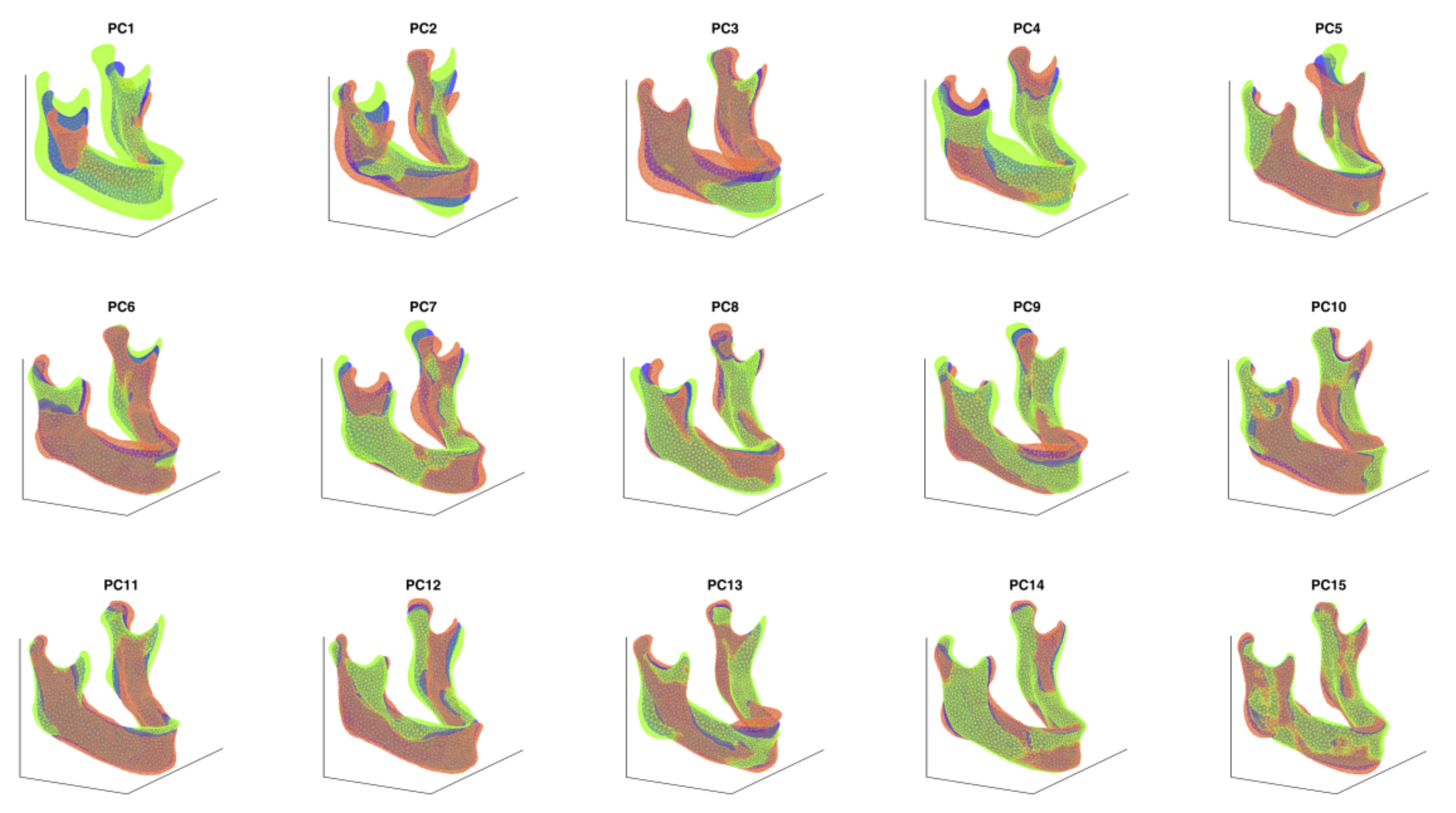
The different PCs describing the main shape variations with reference to the average shape are illustrated in Figure 3 and Figure 4 for the mandible and for the femur, respectively. The respective animations are reported as Supplementary Materials.

Following the definition of the SSM (Equation (6)), each ith PC contributes to determine the geometry of each bone sample with a certain weight W_i. Hence, the frequency distributions of these weights among the whole analyzed cohort can be considered. Figure 5a shows them with reference to the mandible’s dataset. It is evident that the normality of distributions is quite questionable. For this reason, the authors chose to develop a stochastic model based on empirical cumulative frequency distributions (Figure 5b).

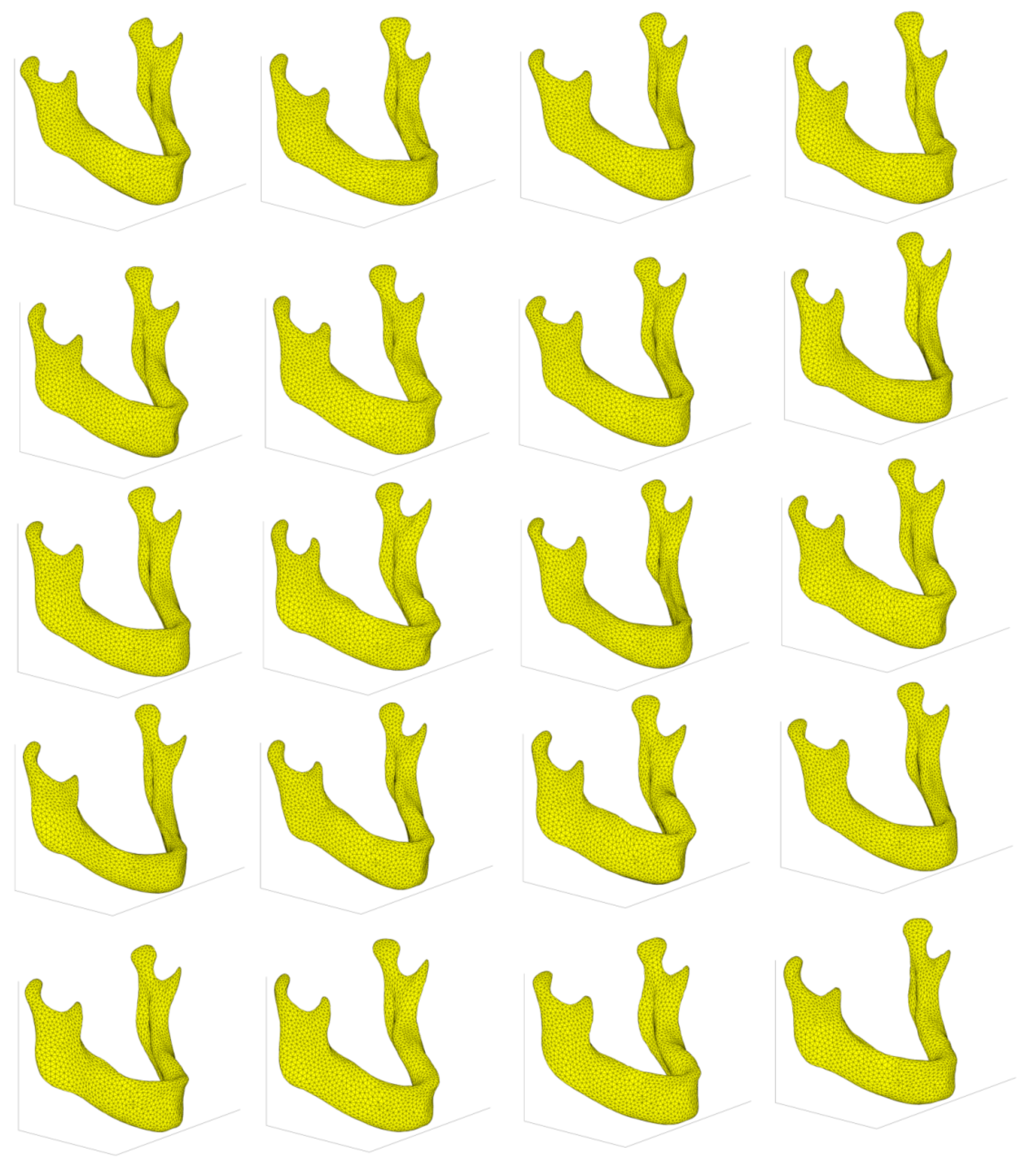
New sets of 20 bones, the size having been defined arbitrarily for example purposes, could therefore be generated applying inverse transform sampling for both the mandible and the proximal femur changing the PCs weights; the results are reported in Figure 6 and Figure 7.

4. Discussion

The here presented work was mainly aimed at illustrating the procedure to adopt in order to build an SSM. Two databases referring to two different bone sites were used to illustrate the procedure. The proximal femur database was definitely larger and could therefore be considered more exhaustive compared to the available mandible database, which was more limited. In both cases, PCA proved its efficiency in summarizing the main anatomical features: 40 mandibles were considered, and as a result of PCA, 15 components sufficed to generate a theoretically infinite set of different mandible shapes, able to cover 90% of the variability identified in the original database. As far as the 98 proximal femurs database is concerned, 90% of the shape variance could be covered by nine PCs. The geometry of the proximal femur is certainly simpler compared to a full mandible, and it is not therefore surprising that a smaller number of PCs was required to cover almost the whole variability present in the more numerous database; this aspect is also confirmed from the work of Taylor et al. [20]. From this perspective, the number of PCs is actually a measure of the geometric shape complexity [21].

The generation of new geometries must follow the empirically estimated frequency distributions of weight components, in order that the actual variability found in nature is reproduced. The hypothesis of a normal distribution is questionable according to the results that were obtained: therefore, the authors preferred to avoid fitting the cumulative frequency with a known statistical distribution. If statistical tests were performed to check weight distributions normality, this statistical hypothesis would not be rejected in most cases. However, it is well known that failure to reject statistical hypothesis does not mean, as assumed by some authors, that the normality of the distribution has been demonstrated [22]: the approach followed herein by the authors was therefore certainly considered more precautionary.

The possibility to create a statistically sound set of bones is a mandatory issue when, for instance, a prosthesis needs to be designed to cover the need of a whole population [23]. In addition, it can provide key information for the design of parametric [24] and modular [25] models. Three-dimensional models can also be used to create patient-specific finite element models [6,26] or multibody models in order to study the structural behaviour of a prosthesis or of a synthesis device [27,28]: in this whole context, working on iso-topological meshes allows straightforward applications in the setup of numerical procedures, without additional need for technical skills.

Statistical shape models might also be used for diagnostic purposes, in order to assess if a certain morphology could be considered as “normal”, checking if it falls inside a given probability range [29] as well as more deeply investigating relations between anatomy and a number of pathologies [30,31,32].

The application of the SSM method was presented here to also consider the possibility of predicting of new bone shapes. It must be said that CT scan data allows not only the three-dimensional reconstruction of external and internal anatomical structures, but also the extrapolation of information on material mechanical properties [30,33,34]. In this context, when dealing with bones, the possibility to generate new instances enables us to gather not only the shape but also the local density that may indeed be preferable, in order to have a full bone model for further investigations (i.e., static and dynamic analyses). To this end, the same approach presented here might be also adopted for carrying out PCA on the patient-specific local density values from the CT Hounsfield Units, so that the prediction of the mechanical properties of new mandible and femur bone instances would also be allowed. Thanks to the availability of CT images for the two bone districts analysed here, this will in fact represent the next step to be tackled, so that the generation of new bone instances gathering shape and density values will be made possible. The stochastic geometric models created within this study and presented here are available for the whole scientific community:

https://www.ing.unipg.it/en/research/industrial-bioengineering ‘Shared Files’ (accessed on 2 June 2021)

http://www.biomedlab.polito.it/en/research/biomechanics (accessed on 2 June 2021)

Geometrical models will be made available upon request, according to the experimental cumulative density functions.

References

1. Ambu, R.; Motta, A.; Calì, M. Design of a Customized Neck Orthosis for FDM Manufacturing with a New Sustainable Bio-composite. In Proceedings of the Design Tools and Methods in Industrial Engineering, Modena, Italy, 9–10 September 2019; Rizzi, C., Andrisano, A.O., Leali, F., Gherardini, F., Pini, F., Vergnano, A., Eds.; Springer International Publishing: Cham, Switzerland, 2020; pp. 707–718. [Google Scholar]
2. Stephen, J.M.; Calder, J.D.F.; Williams, A.; El Daou, H. Comparative accuracy of lower limb bone geometry determined using MRI, CT, and direct bone 3D models. J. Orthop. Res. 2020. [Google Scholar] [CrossRef]
3. Lalone, E.A.; Willing, R.T.; Shannon, H.L.; King, G.J.W.; Johnson, J.A. Accuracy assessment of 3D bone reconstructions using CT: An intro comparison. Med. Eng. Phys. 2015, 37, 729–738. [Google Scholar] [CrossRef] [PubMed]
4. Aldieri, A.; Terzini, M.; Osella, G.; Priola, A.M.; Angeli, A.; Veltri, A.; Audenino, A.L.; Bignardi, C. Osteoporotic Hip Fracture Prediction: Is T-Score-Based Criterion Enough? A Hip Structural Analysis-Based Model. J. Biomech. Eng. 2018, 140. [Google Scholar] [CrossRef]
5. Galibarov, P.E.; Prendergast, P.J.; Lennon, A.B. A method to reconstruct patient-specific proximal femur surface models from planar pre-operative radiographs. Med. Eng. Phys. 2010, 32, 1180–1188. [Google Scholar] [CrossRef] [PubMed]
6. Schmutz, B.; Reynolds, K.J.; Slavotinek, J.P. Customization of a generic 3D model of the distal femur using diagnostic radiographs. J. Med. Eng. Technol. 2008, 32, 156–161. [Google Scholar] [CrossRef] [Green Version]
7. Noble, P.C.; Alexander, J.W.; Lindahl, L.J.; Yew, D.T.; Granberry, W.M.; Tullos, H.S. The anatomic basis of femoral component design. Clin. Orthop. Relat. Res. 1988, 148–165. [Google Scholar] [CrossRef]
8. Zanetti, E.M.; Crupi, V.; Bignardi, C.; Calderale, P.M. Radiograph-based femur morphing method. Med. Biol. Eng. Comput. 2005, 43, 181–188. [Google Scholar] [CrossRef] [PubMed]
9. Brunton, A.; Salazar, A.; Bolkart, T.; Wuhrer, S. Review of statistical shape spaces for 3D data with comparative analysis for human faces. Comput. Vis. Image Underst. 2014, 128, 1–17. [Google Scholar] [CrossRef] [Green Version]
10. Yang, L.; Udall, W.J.M.; McCloskey, E.V.; Eastell, R. Distribution of bone density and cortical thickness in the proximal femur and their association with hip fracture in postmenopausal women: A quantitative computed tomography study. Osteoporos. Int. 2014, 25, 251–263. [Google Scholar] [CrossRef]
11. Qasim, M.; Farinella, G.; Zhang, J.; Li, X.; Yang, L.; Eastell, R.; Viceconti, M. Patient-specific finite element estimated femur strength as a predictor of the risk of hip fracture: The effect of methodological determinants. Osteoporos. Int. 2016, 27, 2815–2822. [Google Scholar] [CrossRef] [Green Version]
12. Hufnagel, H. A Probabilistic Framework for Point-Based Shape Modeling in Medical Image Analysis; Vieweg+Teubner Verlag: Wiesbaden, Germany, 2011; ISBN 9783834817228. [Google Scholar]
13. Zheng, G.; Li, S.; Székely, G. Statistical Shape and Deformation Analysis; Academic Press: New York, NY, USA, 2017; ISBN 9780128127315. [Google Scholar]
14. Pascoletti, G.; Calì, M.; Bignardi, C.; Conti, P.; Zanetti, E.M. Mandible Morphing through Principal Components Analysis. In Proceedings of the International Conference on Design Tools and Methods in Industrial Engineering, Modena, Italy, 9–10 September 2019; pp. 15–23. [Google Scholar]
15. Biancolini, M.E.; Chiappa, A.; Giorgetti, F.; Porziani, S.; Rochette, M. Radial basis functions mesh morphing for the analysis of cracks propagation. Procedia Struct. Integr. 2018, 8, 433–443. [Google Scholar]
16. Biancolini, M.E. Fast Radial Basis Functions for Engineering Applications; Springer International Publishing: Cham, Switzerland, 2018; ISBN 9783319750118. [Google Scholar]
17. Grassi, L.; Hraiech, N.; Schileo, E.; Ansaloni, M.; Rochette, M.; Viceconti, M. Evaluation of the generality and accuracy of a new mesh morphing procedure for the human femur. Med. Eng. Phys. 2011, 33, 112–120. [Google Scholar] [CrossRef] [Green Version]
18. Veneziano, A.; Landi, F.; Profico, A. Surface smoothing, decimation, and their effects on 3D biological specimens. Am. J. Phys. Anthropol. 2018, 166, 473–480. [Google Scholar] [CrossRef]
19. Gower, J.C. Generalized procrustes analysis. Psychometrika 1975, 40, 33–51. [Google Scholar] [CrossRef]
20. Taylor, M.; Viceconti, M.; Bhattacharya, P.; Li, X. Finite element analysis informed variable selection for femoral fracture risk prediction. J. Mech. Behav. Biomed. Mater. 2021, 118, 104434. [Google Scholar] [CrossRef] [PubMed]
21. Skaudickas, D.; Veikutis, V.; Vitkus, A.; Peciulytė, G.; Marciulionyte, D.; Sakalyte, G.; Krisciukaitis, A.; Vaitiekaitis, G. Evaluation of complexity of induced necrosis zone shape by means of principal component analysis. J. Vibroeng. 2014, 16, 4115–4125. [Google Scholar]
22. Morrison, S.J. Statistics for Engineers: An Introduction; Wiley: New York, NY, USA, 2009; ISBN 9780470745564. [Google Scholar]
23. Meynen, A.; Matthews, H.; Nauwelaers, N.; Claes, P.; Mulier, M.; Scheys, L. Accurate reconstructions of pelvic defects and discontinuities using statistical shape models. Comput. Methods Biomech. Biomed. Eng. 2020, 23, 1026–1033. [Google Scholar] [CrossRef] [PubMed]
24. Chen, X. Parametric design of patient-specific fixation plates for distal femur fractures. Proc. Inst. Mech. Eng. Part H J. Eng. Med. 2018, 232, 901–911. [Google Scholar] [CrossRef] [PubMed]
25. Voskuil, R.T.; Mayerson, J.L.; Scharschmidt, T.J. Management of Metastatic Disease of the Upper Extremity. J. Am. Acad. Orthop. Surg. 2021, 29, e116–e125. [Google Scholar] [CrossRef]
26. Xiao, D.; Lian, C.; Wang, L.; Deng, H.; Lin, H.Y.; Thung, K.H.; Zhu, J.; Yuan, P.; Perez, L.; Gateno, J.; et al. Estimating Reference Shape Model for Personalized Surgical Reconstruction of Craniomaxillofacial Defects. IEEE Trans. Biomed. Eng. 2021, 68, 362–373. [Google Scholar] [CrossRef]
27. Pascoletti, G.; Cianetti, F.; Putame, G.; Terzini, M.; Zanetti, E.M. Numerical simulation of an intramedullary Elastic Nail: Expansion phase and load-bearing behavior. Front. Bioeng. Biotechnol. 2018, 6, 174. [Google Scholar] [CrossRef] [Green Version]
28. Putame, G.; Pascoletti, G.; Terzini, M.; Zanetti, E.M.; Audenino, A.L. Mechanical Behavior of Elastic Self-Locking Nails for Intramedullary Fracture Fixation: A Numerical Analysis of Innovative Nail Designs. Front. Bioeng. Biotechnol. 2020, 8, 557. [Google Scholar] [CrossRef]
29. Heutinck, P.; Knoops, P.; Florez, N.R.; Biffi, B.; Breakey, W.; James, G.; Koudstaal, M.; Schievano, S.; Dunaway, D.; Jeelani, O.; et al. Statistical shape modelling for the analysis of head shape variations. J. Cranio-Maxillofac. Surg. 2021, 49, 449–455. [Google Scholar] [CrossRef]
30. Aldieri, A.; Terzini, M.; Audenino, A.L.; Bignardi, C.; Morbiducci, U. Combining shape and intensity dxa-based statistical approaches for osteoporotic HIP fracture risk assessment. Comput. Biol. Med. 2020, 127, 104093. [Google Scholar] [CrossRef] [PubMed]
31. Bredbenner, T.L.; Eliason, T.D.; Potter, R.S.; Mason, R.L.; Havill, L.M.; Nicolella, D.P. Statistical shape modeling describes variation in tibia and femur surface geometry between Control and Incidence groups from the Osteoarthritis Initiative database. J. Biomech. 2010, 43, 1780–1786. [Google Scholar] [CrossRef] [PubMed] [Green Version]
32. McLeod, K.; Mansi, T.; Sermesant, M.; Pongiglione, G.; Pennec, X. Statistical shape analysis of surfaces in medical images applied to the tetralogy of fallot heart. In Modeling in Computational Biology and Biomedicine: A Multidisciplinary Endeavor; Springer: Berlin/Heidelberg, Germany, 2013; ISBN 9783642312083. [Google Scholar]
33. Goda, I.; Rahouadj, R.; Ganghoffer, J.-F.; Kerdjoudj, H.; Siad, L. 3D couple-stress moduli of porous polymeric biomaterials using µCT image stack and FE characterization. Int. J. Eng. Sci. 2016, 100, 25–44. [Google Scholar] [CrossRef]
34. Louna, Z.; Goda, I.; Ganghoffer, J.-F. Homogenized strain gradient remodeling model for trabecular bone microstructures. Contin. Mech. Thermodyn. 2019, 31, 1339–1367. [Google Scholar] [CrossRef]
Figure 1. A schematic workflow gathering the steps of the whole procedure: mesh morphing, Generalized Procrustes Analysis (GPA), Principal Component Analysis (PCA), Statistical Shape Model (SSM) and stochastic model.
Applsci 11 05204 g001
Figure 2. Cumulative explained variance versus the number of principal components for the mandible (a) and for the proximal femur (b).
Applsci 11 05204 g002
Figure 3. The first 15 mandible principal components (PCs). The average mandible shape is represented in blue, while the deformations along the ith PC applying a weight equal to ± λ i are reported in green/brown.
Applsci 11 05204 g003
Figure 4. The first nine proximal femurs principal components (PCs). The average femur shape is represented in blue, while the deformations along the ith PC applying a weight equal to ± λ i are reported in green/brown.
Applsci 11 05204 g004
Figure 5. Empirical Frequency (a) and cumulative frequency (b) distributions of weights for each principal component, with reference to the 40 mandibles set.
Applsci 11 05204 g005
Figure 6. New set of 20 mandibles, generated through inverse transform sampling, applied on empirical cumulative weight distribution of weights for each component.
Applsci 11 05204 g006
Figure 7. New set of 20 femurs, generated through inverse transform sampling, applied on empirical cumulative weight distribution of weights for each component.
Applsci 11 05204 g007