Application Feature
Postoperative magnetic resonance imaging (MRI) evaluation of ACL graft maturity is a useful tool to predict graft insufficiency and may influence clinical decisions regarding patient return to full intensity sports activity.
Abstract
Background: Postoperative magnetic resonance imaging (MRI) evaluation of anterior cruciate ligament (ACL) graft maturity is a useful and practical tool that allows for assessment of graft status and remodeling stage. The purpose of this study was to evaluate and compare previously described methods of graft evaluation in MRI. We identify factors influencing the maturation and correlating graft appearance in MRI with indirect symptoms of graft insufficiency to identify patients at risk. Methods: Retrospective evaluation was performed in 44 patients who received bone patellar tendon bone (BPTB) ACL reconstruction with nine consecutive postoperative MRIs at 2, 6, 12, 18, 24, 36, 48, 72, and 96 weeks. Graft status was evaluated using signal-to-noise quotient (SNQ) methods in both sagittal and axial planes. We also assessed the homogeneity of the graft by standard deviation (SD) of signal intensity. SNQ was correlated with patient’s age, sex, postoperative weight-bearing, as well as indirect signs of graft insufficiency by MRI including graft appearance, posterior cruciate ligament (PCL) buckling, and measurement of anterior tibia subluxation. Results: We observed that the results of modelling SNQs from both sagittal and axial planes were similar. For both SNQs, the change over weeks quotient was nonlinear where the clinical parameter increased at week 36 and subsequently decreased. The SNQ at week 96 does not reach the levels from week 2. We observed that the model incorporating SNQ and relative SD (rSD) in the sagittal plane predicted the tibia anterior subluxation proportions better than the model with clinical parameters measured in the axial plane. Our results demonstrate that greater SD is associated with less graft homogeneity, which could indicate that this model is a good predictor of graft insufficiency. In addition, the proportion of PCL buckling increased over the course of the study. Conclusions: MRI graft evaluation is very useful for assessing graft ligamentization stage and to predict graft insufficiency.
1. Introduction
Anterior cruciate ligament (ACL) rupture causes knee instability, which affects sport activities and increases the risk of meniscal injury and early osteoarthrosis [1]. ACL reconstruction reduces anterior tibial laxity but does not fully restore normal tibiofemoral kinematics [2]. Despite efforts and significant advances in ACL reconstruction, clinical failures continue to occur [3]. It is still debated among researchers and clinicians on what processes are involved in ACL graft healing and remodeling and how long these processes take in patients [4]. This information is crucial for patients to return to sports activities.
Claes et al. [5] performed a systematic review of literature on the “ligamentization” process of human ACL graft. He showed that a free tendon graft used for ACL reconstruction undergoes a series of biologic processes called “ligamentization”. Ligamentization may be divided further into the early phase, remodeling, and maturation of the graft. The graft shows viability throughout the whole process. In histopathologic evaluation, the graft resembles a normal intact human ACL. However, specific differences exist between the phases. In addition, there is no consensus for the exact time frames for each stage of the ligamentization process.
Biercevicz et al. [6] proved that volume and greyscale values are predictive of the healing graft’s structural properties in his preclinical animal model studies. He also showed magnetic resonance imaging (MRI) parameters may predict biomechanical properties and outcome measurements in human patients after ACL reconstruction [7]. Weiler et al. [8] also showed in an animal model that quantitative evaluation of MRI might be a useful tool for following the graft remodeling. Dong et al. [4] proved that implanted grafts could transform into native ACL-like tissue with a similar ultrastructure and metabolism.
The aim of our study was to evaluate the bone-patellar tendon-bone (BPTB) ACL graft remodeling process in our group of patients. We used previously described techniques to evaluate their efficacy. Our results were correlated with variables including age, sex, and weight-bearing. Additionally, for the first time to our knowledge, we correlated the graft remodeling process not only with clinical outcome, but also with indirect MRI signs of ACL graft insufficiency. We also analyzed standard deviation of SI as a separate value.
2. Materials and Methods
Our retrospective analysis included 44 patients who underwent BPTB ACL reconstruction in our hospital between December 2011 and March 2015. There were 23 males and 21 females. The mean age of patients was 28 years old (range 13–73). There were 18 right and 26 left knees. At the time of final evaluation (96 weeks postoperatively), all patients, except one, were stable on clinical evaluation. This patient with ACL graft complete injury had a traumatic secondary graft failure.
The rehabilitation protocol was the same for all patients. The only difference was weight-bearing immediately after the surgery, and this factor was also evaluated separately in this study. One group of patients had full weight-bearing immediately after the surgery. The second group had no weight bearing for the first three weeks after the surgery. A brief description of the rehabilitation protocol is presented in Table 1.

Table 1.
Brief description of rehabilitation protocol.
MRI was performed in all patients postoperatively at 2, 6, 12, 18, 24, 36, 48, 72, and 96 weeks. MRI images were obtained using a 1.5 tesla GE Signa HDxt scanner with an 8-channel knee coil. Full, routine MRI protocol for ACL assessment included axial and sagittal PDWI (Proton Density Weighted Images), axial FSE STIR (Fast Spin Echo Short Tau Inversion Recovery), DWI (Diffusion Weighted Images), and T2 Mapping sequences.
Signal intensity was measured manually using the regions of interest (ROI) tool with a diameter of 3 mm on axial and sagittal PDWI sequences (Table 2).
Table 2.
Magnetic resonance imaging (MRI) parameters.
To measure ACL graft signal intensity, we used the method previously described by Howell et al. [9], Ahn et al. [10] and Vogl et al. [11], by calculating signal-to-noise quotient (SNQ, Equation (1)):
We wanted to evaluate which measurements (sagittal or axial plane) are more reliable for predicting ACL graft insufficiency. Therefore, we calculated separately for both planes.
We also evaluated age, sex, immediate postoperative weight-bearing, and intraoperative tensioning of the graft, which is the initial position of the tibia in relation to the femur.
The lower value of SNQ—the better graft appearance, the better mechanical properties of the graft and the more comparable ACL graft is to posterior cruciate ligament (PCL) healthy ligament.
2.1. Measurement on the Sagittal Plane
A sagittal plane in the PDWI sequence with the best visibility of the ACL graft was chosen for evaluation. We manually drew ROI (diameter of 3 mm) in 1/3 distal and 1/3 midsubstance of the graft graft, PCL, and the background (1 cm distal from the tip of the patella and 1 cm anterior to the skin) (Figure 1). The SNQ for this plane was calculated by averaging SNQs calculated separately from the two measurements.
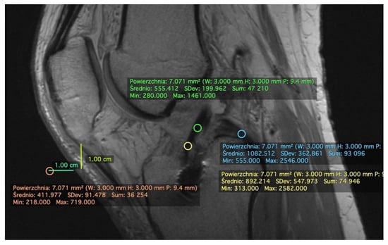
Figure 1.
Measurement of signal intensity on PDWI sagittal plane. Example measurements of patient #5 at 2 weeks postoperatively. We manually drew a region of interest (ROI) in 1/3 distal (yellow oval) and 1/3 midsubstance (green oval) of anterior cruciate ligament (ACL) graft, posterior cruciate ligament (PCL, blue oval), and the background (1 cm distal from the tip of the patella and 1 cm anterior to the skin) (orange oval). The mean values were later put to Equation (1) and used to calculate signal-to-noise quotient (SNQ). The standard deviation (SD) values were used to calculate relative SD (rSD) with Equation (2).
2.2. Measurement on the Axial Plane
The lowest most distal level of the intercondylar notch was chosen for measuring the axial plane. ROI (diameter of 3 mm) was drawn on ACL graft, PCL, and background (1 cm anterior to the skin on the knee’s anterior aspect) (Figure 2). SNQ was calculated using Equation (1).
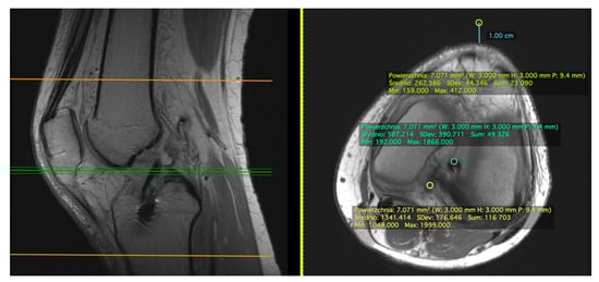
Figure 2.
Measurement of signal intensity on PDWI axial plane. Example measurements of patient #5 at 2 weeks postoperatively. We manually drew ROI (diameter of 3 mm) of ACL graft (green oval), PCL (yellow oval), and the background (1 cm anterior to the anterior aspect of the knee) (light green oval).
2.3. Standard Deviation (SD)
We evaluated the standard deviation (SD) of each measurement as a separate value. Since SD represents average difference from the mean value, lower SD indicates that the values within the ROI are more similar to the mean value, thus the graft is more homogenous. Similarly, higher SD indicates more heterogenous graft. To incorporate standard deviations of the ACL graft signal intensity, we computed relative SD index (rSD, Equation (2)):
For the measurements from the sagittal plane, a sum of the two measurements was used in the numerator.
2.4. Indirect Signs of Anterior Cruciate Ligament (ACL) Graft Insufficiency
We indirectly evaluated ACL graft insufficiency and correlated our findings with other parameters. Parameters taken into consideration were:
- −
- ACL graft appearance: normal/injured (Figure 3a,b)
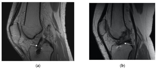 Figure 3. Appearance of the ACL graft (marked with with arrow). (a) Normal (b) injured.
 - −
- PCL appearance: normal buckling (Figure 4a,b)
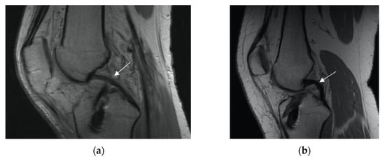 Figure 4. PCL appearance (marked with white arrow): (a) normal, (b) buckling.
 - −
- anterior tibia subluxation (Figure 5)
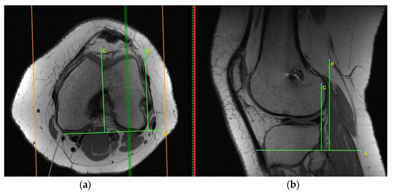 Figure 5. Anterior tibia subluxation. Axial and sagittal image are merged ((a) and the cortex adjacent to PCL in the femoral notch (b)). Measurement of anterior tibial subluxation was made in the sagittal plane (b) at a location midway between the cortex adjacent to PCL in the femoral notch and the most lateral slice containing the lateral femoral condyle (marked on axial plane, (a)). The degree of tibial subluxation was measured by the distance between those two lines in millimeters (between lines B and C, (b)).
Measurement of anterior tibial subluxation was made in the sagittal plane at a location midway between the cortex adjacent to PCL in the femoral notch and the most lateral slice containing the lateral femoral condyle. In Figure 5, two vertical lines were drawn tangential to the posterior cortical margin of the lateral femoral condyle and the lateral tibial condyle. Both lines were drawn parallel to the margin of the image frame. The degree of tibial subluxation was measured by the distance between the two lines in millimeters. Anterior tibia subluxation was evaluated as (+), and posterior tibia subluxation (in relation to femur position) as (−).
2.5. Data Analysis
Statistical Analyses
We used R 4.0.2 [12] for performing statistical analyses. To analyze changes in SNQs and indirect signs of ACL graft insufficiency over postoperative timepoints and their relationships to rSDs, sex, age, and weight bearing, a series of Bayesian multilevel regression was conducted with intercepts allowed to vary by patient. Details of the models are provided with the results. All continuous variables were entered into the models after transformation to Z-scale and categorical predictors were coded with orthogonal sum to zero contrasts. Change over weeks (week predictor) was modelled with orthogonal quadratic polynomial, which allowed us to capture non-linear trend in change of the parameters. For all categorical predictors, an interaction with week predictor was also investigated to test whether the change over weeks depended on these predictors. Each model was estimated separately for measurement made in sagittal and axial planes.
In Bayesian statistics, the inference is based on analyzing posterior probability distributions of model parameters (e.g., regression weight of week predictor), obtained by integrating likelihood with prior probability distributions of the model parameters. The model parameter is statistically credible when 95% of credible intervals (CI) of the posterior distribution exclude zero [13]. As a point estimate of the effect, medians of the posterior distributions are presented. As priors for all regression weights, non-informative, standard normal distributions were used (i.e., with M = 0 and SD = 1).
To present expected values of clinical parameters, we provide posterior predicted marginal means for SNQs and PCL subluxation and probabilities for overall graft state and PCL anterior subluxation. These values were computed from model parameters and can be thought of as better summary statistics than simple descriptive statistics, since they incorporate all the uncertainty in the data and model.
For models with continuous dependent variables, Bayesian R2 [14] was provided as a measure of model fit. Therefore, prediction accuracy was reported for models with categorical dependent variables. Both statistics are in the range zero to one, with one indicating perfect model fit.
To approximate posterior distributions of the models, a Markov Chain Monte Carlo (MCMC) sampling procedure was conducted using the brms (Bayesian Regression Models using ‘Stan’) package [15]. For each reported model, six parallel MCMC chains were used. Each chain consisted of 6000 samples, with 3000 samples used as warmup period and every 10th sample recorded, which resulted in a total of 1800 recorded samples. Efficient sampling procedures resulted in well-mixed and autocorrelation-free chains and unimodal posteriors.
3. Results
3.1. Remodeling Process of the ACL Graft
The Bayesian multilevel skew-normal regression was used to model SNQs. Skew-normal distribution was used to control for any skewness observed in the data. Multilevel structure was used to control for differences between patient average SNQ values and patient variability. Model coefficients are presented in Table 3. Selected predicted posterior means of SNQ measurements in the sagittal plane are presented on Figure 6.
Table 3.
Results of Bayesian multilevel skew-normal regressions of SNQs measured at sagittal and axial planes as dependent variables.
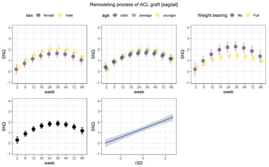
Figure 6.
Remodeling process of ACL graft. Note SNQ has a non-linear structure. SNQ increased until week 36, suggesting the worsening of the ACL graft. Later SNQ decreased until the final timepoint (week 96), but never was as low as the SNQ of week 2 There were no significant differences between males and females in any age groups. Posterior predicted marginal means (points or blue line) of the SNQ parameter measured at the sagittal plane. The vertical lines and shaded area show 95% credible interval. The y-axis limits span over the range of middle 95% of the data.
The results of modelling SNQs from both sagittal and axial planes were similar. For both SNQs, the change over weeks value had a nonlinear nature where the clinical parameter increased until week 36 and then decreased. Our results of predicted means demonstrated that the SNQ at week 96 does not reach the level from week 2 (Figure 6). In addition, both SNQs were moderately and positively correlated to the corresponding rSD indices, indicating that increase in rSD was associated with increase in SNQ. SD represents a measure of the amount of variation or dispersion of a set of values. Therefore, we assumed greater SD is associated with less graft homogeneity.
The change of SNQ over weeks was weakly dependent on weight bearing, for measurements in the sagittal plane. The initial increase in SNQ values was noticeably lower among patients who fully weighted their leg from the beginning. In addition, SNQ change was also related to age, where the increase in parameter values slightly higher among younger patients.
3.2. Indirect Signs of ACL Graft Insufficiency
Next, we modelled indirect signs of ACL graft insufficiency. The SNQ indices were constituted as predictors. We ran separate models with measurements from sagittal and axial planes. This allowed us to test which measurement constituted better proxy for indirect signs of insufficiency while controlling for possible associations with remaining factors included in the study. To test this, we compared models that included SNQ and rSD measured in the sagittal plane with a models in the axial plane using a logarithm of the Bayes factor (BF). The BF value range from –1 to 1 indicates no credible differences between the models. Values below −1 or above 1 indicate that the model in the denominator or in the numerator should be preferred, respectively.
3.2.1. Overall Graft State
To model overall graft state, Bayesian multilevel logistic regression with varying intercepts across patients was used. Model coefficients are presented in Table 4 and selected predicted posterior proportions are presented in Figure 7. Since the injured state was coded as the event, the posterior predicted probabilities in Figure 2 should be interpreted as predicted proportions of patients assessed with injured grafts.
Table 4.
Results of Bayesian multilevel logistic regressions with graft state as the dependent variable.
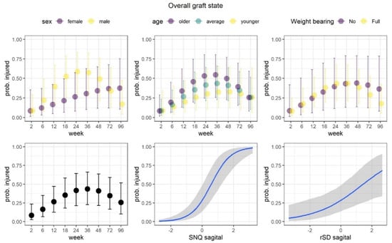
Figure 7.
Overall graft state. The proportion of injured grafts changed non-linearly over the course of the study, with the highest values at 36 weeks. The proportions steadily increased over the course of the study in female patients, while the proportions increased rapidly up to week 24 and then rapidly decreased in male patients. At week 96, the proportions came close to the level observed at week 2 in male patients. Posterior predicted marginal proportions (points or blue lines) of the injured grafts. The vertical lines and shaded area show 95% credible interval.
We observed that the model that incorporated SNQ and rSD at the sagittal plane predicted the proportions of injured grafts better than the model measuring the axial plane (BF = 1.922). Thus, we focused on the results from the better model. The proportion of injured grafts changed non-linearly over the course of the study, with the highest value at 36 weeks. Statistically credible relations were observed for both SNQ and rSD, which demonstrated increase in these indices was associated with an increase in the proportion of injured grafts. The association was much stronger for the SNQ index. Finally, a high difference between men and women was observed in regard to change in proportions over the weeks. The proportions steadily increased over the course of the study in female patients, while the proportions increased rapidly up to week 24 and then rapidly decreased in male patients. At week 96, the proportions came close to the level observed at week 2 in male patients. The effects of weight-bearing and age were not statistically credible.
3.2.2. Posterior Cruciate Ligament (PCL) Buckling (Subluxation)
To model PCL buckling, Bayesian multilevel logistic regression with varying intercept across patients was used. Model coefficients are presented in Table 5 and selected posterior predicted proportions are presented in Figure 8. Since the subluxated state was coded as the event, the posterior predicted probabilities in Figure 8 should be interpreted as predicted proportions of patients with subluxation.
Table 5.
Results of Bayesian multilevel logistic regressions with anterior tibia subluxation as the dependent variable.
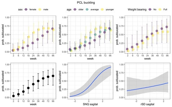
Figure 8.
PCL buckling. We observed statistically credible and positive association with SNQ values for PCL buckling. As the SNQ values increased, the proportion of subluxated PCLs also increased. Additionally, the nonlinear part of the change over weeks was credibly dependent on the age of patients. Among older and average ages patients, the proportion increased steadily, while among younger patients it increased more rapidly (up to week 48) and then decreased. The effects of weight bearing, sex and rSD were not statistically credible. Posterior predicted marginal proportions (points or blue lines) of the PCL subluxation. The vertical lines and shaded area show 95% credible interval.
We observed that the model that incorporated SNQ and rSD in the sagittal plane predicted proportions of PCL buckling better than the model in the axial plane (BF = 12.21). Thus, we focus on the results from this model next. The proportion the PCL subluxation increased over the course of the study (note that the main effect of the quadratic trend is not statistically credible). We observed statistical credible and positive association with SNQ. As the SNQ values increased, the proportion of subluxated PCLs also increased. Additionally, the non-linear part of change over weeks was dependent on the age. The proportions increased steadily in older and average-aged patients while they increased more rapidly and decreased in younger patients. The effects of weight bearing, sex, and rSD were not statistically credible.
3.2.3. Anterior Tibia Subluxation
To model the anterior tibia subluxation, we used Bayesian multilevel skew-normal regression. Differences between average anterior tibia subluxation of patients and their variability were controlled. Additional control of variability of anterior tibia subluxation over the weeks was incorporated. In these analyses we also incorporated additional predictor, which grouped patients according to the anterior tibia subluxation value at week 2: patients with negative subluxation (meaning posterior tibia subluxation in relation to femoral condyles) constituted one group, and remaining patients constituted another group.
For this indirect sign of the ACL graft insufficiency, we did not observe statistically credible differences between models SNQ and rSD measured at the sagittal plane or axial plane, BF = 0.74. We incorporated an additional predictor by grouping patients according to the anterior tibia subluxation value at week 2: (1) patients with negative subluxation (posterior tibia subluxation in relation to femoral condyles), and (2) remaining patients. Model coefficients are presented in Table 6 and selected predicted posterior means of anterior tibial subluxation are presented in Figure 9.
Table 6.
Results of Bayesian multilevel skew- normal regressions with PCL subluxation as the dependent variable.
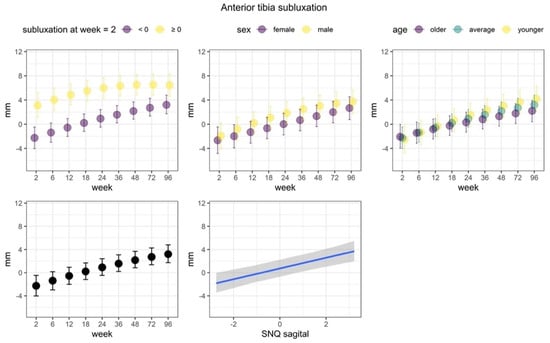
Figure 9.
Anterior tibia subluxation. We observed that anterior tibia subluxation increased over the course of the study. Most importantly, we observed statistically credible differences of the anterior tibia subluxation state at week 2. Average subluxation was lower among patients who started with negative subluxation. In addition, the linear increase was noticeably stronger among this group of patients, as compared to patients who had nonnegative subluxation at week 2. Posterior predicted marginal means (points or blue line) of the PCL subluxation. The vertical lines and shaded area show 95% credible interval. The y-axis limits span over the range of middle 95% of the data.
We observed that anterior tibia subluxation mainly increased over the course of the study. The non-linear trend of the week predictor was also statistically credible, but relatively small, which indicated a slightly lower increase of the subluxation in the last weeks of the study. The SNQ index was credibly and positively associated with subluxation, although the relationship was rather weak. The linear increase over the weeks was weakly associated to age, where increases were more apparent in younger patients. Most importantly, we observed statistically credible differences of the anterior tibia subluxation state at week 2. Average subluxation was lower among patients who started with negative subluxation. In addition, the linear increase was noticeably stronger among this group of patients, as compared to patients who had non-negative subluxation at week 2.
4. Discussion
To the best of our knowledge, this is the first complex study evaluating ACL graft maturity by comparing different methods for measuring graft signal intensity, homogeneity of the graft, and evaluating the effect of sex, age, and weight-bearing being believed to have an impact on graft maturity. Moreover, we studied indirect MRI’s signs of ACL graft insufficiency and its relationship to signal intensity.
In 2019 Van Dyck et al. [16] performed a systematic review of papers assessing ACL graft maturation in MRI studies. He concluded that methods used across studies were too heterogeneous to conclude time frames of signal intensity. The signal intensity of the graft was poorly correlated with clinical outcomes.
Van Groningen et al. [17] published a systematic review of papers assessing ACL graft maturity. He identified 10 studies with serial MRI measurements of SNQ including 479 patients (20–98 patients per study). Semi-tendinous and gracilis tendons were used for ACL reconstruction (six studies), quadriceps tendon (one study), and bone-patellar tendon-bone grafts (3 studies). Allografts were used in three studies, apart from autografts. In all studies, SNQ was calculated either by comparing signal intensity of the graft to the posterior cruciate ligament or the background. Based on available data, Van Groningen concluded that MRI SNQ was the highest at six months postoperatively and later had a gradual decrease over time. However, in his opinion, the MRI SNQ method should not be used to predict graft maturity and functional and clinical outcomes.
In our study we verified different methods for evaluating ACL graft maturity: ROI and SNQ methods on axial and sagittal plane as well as rSD values. It is the first study to compare measurements obtained in both sagittal and axial planes. We showed that average values from two measurements of ACL graft taken in the sagittal plane best represent graft status. We also determined the SD of signal intensity of the graft as a new parameter for graft evaluation and prediction of graft insufficiency. The rSD was related to SNQ and overall grafts state, indicating that graft homogeneity is also an important indicator of graft well-being. We also evaluated the relationship between graft maturity and more subtle signs of ACL graft insufficiency, such as graft status, PCL buckling and exact measurement of anterior tibia subluxation.
Fukuda et al. [18] evaluated SNQ for ACL graft maturation in 10 multisequence MRIs performed within 50 months postoperatively. Forty-five patients with a mean age of 27 years old were included in the prospective study. All patients underwent double-bundle ACL reconstruction. Subsequently, all patients received a MRI at 3 weeks and 6, 9, 12, 18, 24, 36, 48, and 50 months after surgery. In the conclusion of the study, Fukuda stated that at least 18 months was needed for the mean SNQ of the anteromedial bundle for normalization, whereas for the postero-lateral bundle, at least 24 months was needed.
Zaffagnini et al. [19] showed that even though hamstring tendons used for ACL reconstruction undergo a transformation, they do not match the ultrastructure pattern of a native ACL for up to ten years.
In our study, we showed that even at 96 weeks postoperatively, signal intensity of the graft did not match values measured immediately after the reconstruction (at two weeks). Our data suggest that normalization of the signal make take even longer. The question “what would be the best time for patients to return to full sport activity” remains unanswered.
We did not find any significant association between graft maturity and age of the patient at the time of surgery. However, further studies including more heterogeneous groups are needed, as our group of patients was rather young (mean age 28 years old). Sex of the patient did not have an effect on graft maturity. On the other hand, full weight bearing immediately after surgery seemed to improve graft remodeling with smaller values of signal intensity. This finding is in accordance with a study performed by Dziki et al. [20] showing that appropriate mechanical loading improves healing and remodeling process.
Van der List et al. [21] demonstrated that postoperative MRI of the ACL graft might accurately predict the risk of re-rupture of the ACL graft. Our study also presents a good correlation between measured SNQ and secondary symptoms of graft insufficiency.
A particularly interesting finding of this study is that regardless of initial graft tension at the time of surgery, in order to obtain proper positioning of the tibia relative to the femur, the trend of subsequent anterior tibia subluxation remains comparable. Specifically, patients with over-tension (starting with posterior tibia subluxation) end up with smaller degrees of anterior tibia subluxation at 96 weeks. Currently, pre-operative rehabilitation for chronic patients aimed at reducing anterior tibia subluxation might play a key role for final outcome, facilitating proper positioning of the tibia versus femur intraoperatively.
The question regarding the best time to come back to full sports activity remains unanswered, and the literature is conflicting at that point.
Zaffagnini et al. [22] concluded that the best situation would be patient-tailored rehabilitation protocols and return to sport criteria based on individual characteristics. On the other hand, SIGASCOT (Italian Society of Knee, Arthroscopy, Sport, Cartilage and Orthopaedic Technologies) published with Grassi et al. [23] data reflecting on return to sport after ACL reconstruction. 123 SIGASCOT members took part in 14 questions survey focusing, among other things, on return to sport criteria. Returning to non-contact sports was allowed within six months by 87% of members and 53% for contact sports. Return to competitive sport was allowed after six months for 48% for non-contact sports and only 13% for contact sports. The most used criteria to qualify for return to sport were a full range of motion (77%), Lachman test (65%), and Pivot-Shift test (65%). MRI criteria were used only by 12% of surgeons. Nagelli et al. [24] pointed out strong evidence indicating that nearly one-third of younger patients will sustain a second ACL injury within the first two years after ACL reconstruction. He postulates that delaying return to sport for two years after ACL reconstruction will significantly reduce secondary ACL graft injuries. According to Culvenor et al. [25], an accelerated (<10 months) return to sport after ACL reconstruction may be implicated in developing knee osteoarthritis development.
In our opinion, return to sport after ACL reconstruction should individually be assessed based on several factors, where MRI is only one of those:
- −
- Psychological readiness for sport;
- −
- No pain;
- −
- Clinically stable knee (Lachman test, Rollimetr/KT 1000);
- −
- Minimum ROM 0–130;
- −
- MRI—good signal of the graft;
- −
- Biomechanical evaluation: symmetrical muscle strength (on the level of pelvis and knee), good proprioception, movement analysis of simple jump and landing (always paying attention to pelvic stability and valgus knee position). If it is not possible to do an evaluation in the professional lab, a simple, functional test and video analysis based on a cell-phone would also work.
Conflicting data in the literature regarding MRI ACL graft evaluation probably come from the fact that authors tried to use this as a single factor for return to sport assessment or were correlating it with clinical outcome. Return to sport criteria must be multifactorial and lack of correlation of MRI with clinical stability is a positive thing as it may show us more than we may detect with clinical evaluation.
5. Conclusions
MRI examination of ACL graft is an important tool for evaluation of the graft remodeling process. Use of ROI and SNQ measurement techniques on sagittal plane images gives reliable information about graft well-being. Also, rSD was related to SNQ and overall graft state. In our study, none of the ACL grafts returned their baseline postoperative signal intensity (2 weeks) nor did they reach the intensity of a healthy PCL, which ACL grafts were compared to. The worst imaging appearance of an ACL graft in our group was at 36 weeks (about 9 months) postoperatively, at which time the majority of patients around the world would be back to full sport activity. Therefore, one may reconsider the recommended timing for return to full activity. MRI of the graft may also help predict early graft failure and potentially reduce the risk of secondary graft injury by modifying the patient’s activity.
Author Contributions
U.Z.: Conceptualization, methodology, original draft preparation, investigation, visualization. B.C.-Ł.: Conceptualization, methodology, investigation. M.P.: methodology, investigation. M.D.: investigation. K.R.: investigation. K.F.: statistical analysis. Y.C.L.: writing—review and editing. R.Ś.: Conceptualization, investigation. All authors have read and agreed to the published version of the manuscript.
Funding
This research was funded by Science Department, Carolina Medical Center (Pory 78, Warsaw, Poland. www.carolina.pl).
Institutional Review Board Statement
Not applicable.
Informed Consent Statement
Not applicable.
Data Availability Statement
The data presented in this study are available on request from the corresponding author. The data are not publicly available due to limitations set by the Regulation (EU) 2016/679 of the European Parliament and of the Council of 27 April 2016 on the protection of natural persons with regard to the processing of personal data and on the free movement of such data, and repealing Directive 95/46/EC.
Acknowledgments
We would like to thank Izabella Murawska, President of the Management Board of Sport Medica SA for her constant support for Carolina Medical Center Science Department.
Conflicts of Interest
The authors declare no conflict of interest.
References
- Lohmander, L.S.; Englund, P.M.; Dahl, L.L.; Roos, E.M. The Long-Term Consequence of Anterior Cruciate Ligament and Meniscus Injuries: Osteoarthritis. Am. J. Sports Med. 2007, 35, 1756–1769. [Google Scholar] [CrossRef]
- Logan, M.C.; Williams, A.; Lavelle, J.; Gedroyc, W.; Freeman, M. Tibiofemoral Kinematics Following Successful Anterior Cruciate Ligament Reconstruction Using Dynamic Multiple Resonance Imaging. Am. J. Sports Med. 2004, 32, 984–992. [Google Scholar] [CrossRef]
- Condello, V.; Zdanowicz, U.; Di Matteo, B.; Spalding, T.; Gelber, P.E.; Adravanti, P.; Heuberer, P.; Dimmen, S.; Sonnery-Cottet, B.; Hulet, C.; et al. Allograft Tendons Are a Safe and Effective Option for Revision ACL Reconstruction: A Clinical Review. Knee Surg. Sports Traumatol. Arthrosc. 2019, 27, 1771–1781. [Google Scholar] [CrossRef]
- Dong, S.; Xie, G.; Zhang, Y.; Shen, P.; Huangfu, X.; Zhao, J. Ligamentization of Autogenous Hamstring Grafts After Anterior Cruciate Ligament Reconstruction: Midterm Versus Long-Term Results. Am. J. Sports Med. 2015, 43, 1908–1917. [Google Scholar] [CrossRef]
- Claes, S.; Verdonk, P.; Forsyth, R.; Bellemans, J. The “Ligamentization” Process in Anterior Cruciate Ligament Reconstruction: What Happens to the Human Graft? A Systematic Review of the Literature. Am. J. Sports Med. 2011, 39, 2476–2483. [Google Scholar] [CrossRef]
- Biercevicz, A.M.; Miranda, D.L.; Machan, J.T.; Murray, M.M.; Fleming, B.C. In Situ, Noninvasive, T2*-Weighted MRI-Derived Parameters Predict Ex Vivo Structural Properties of an Anterior Cruciate Ligament Reconstruction or Bioenhanced Primary Repair in a Porcine Model. Am. J. Sports Med. 2013, 41, 560–566. [Google Scholar] [CrossRef]
- Biercevicz, A.M.; Akelman, M.R.; Fadale, P.D.; Hulstyn, M.J.; Shalvoy, R.M.; Badger, G.J.; Tung, G.A.; Oksendahl, H.L.; Fleming, B.C. MRI Volume and Signal Intensity of ACL Graft Predict Clinical, Functional, and Patient-Oriented Outcome Measures After ACL Reconstruction. Am. J. Sports Med. 2015, 43, 693–699. [Google Scholar] [CrossRef]
- Weiler, A.; Peters, G.; Mäurer, J.; Unterhauser, F.N.; Südkamp, N.P. Biomechanical Properties and Vascularity of an Anterior Cruciate Ligament Graft Can Be Predicted by Contrast-Enhanced Magnetic Resonance Imaging: A Two-Year Study in Sheep. Am. J. Sports Med. 2001, 29, 751–761. [Google Scholar] [CrossRef]
- Howell, S.M.; Clark, J.A.; Blasier, R.D. Serial Magnetic Resonance Imaging of Hamstring Anterior Cruciate Ligament Autografts during the First Year of Implantation: A Preliminary Study. Am. J. Sports Med. 1991, 19, 42–47. [Google Scholar] [CrossRef]
- Ahn, J.H.; Lee, S.H.; Choi, S.H.; Lim, T.K. Magnetic Resonance Imaging Evaluation of Anterior Cruciate Ligament Reconstruction Using Quadrupled Hamstring Tendon Autografts: Comparison of Remnant Bundle Preservation and Standard Technique. Am. J. Sports Med. 2010, 38, 1768–1777. [Google Scholar] [CrossRef]
- Vogl, T.J.; Schmitt, J.; Lubrich, J.; Hochmuth, K.; Diebold, T.; Del Tredici, K.; Südkamp, N. Reconstructed Anterior Cruciate Ligaments Using Patellar Tendon Ligament Grafts: Diagnostic Value of Contrast-Enhanced MRI in a 2-Year Follow-up Regimen. Eur. Radiol. 2001, 11, 1450–1456. [Google Scholar] [CrossRef] [PubMed]
- Pilson, D.; Decker, K.L. Compensation for Herbivory in Wild Sunflower: Response to Simulated Damage by the Head-Clipping Weevil. Ecology 2002, 83, 3097–3107. [Google Scholar] [CrossRef]
- Kruschke, J.K. Doing Bayesian Data Analysis: A Tutorial with R, JAGS, and Stan; Elsevier: Amsterdam, The Netherlands, 2015; ISBN 978-0-12-405916-0. [Google Scholar]
- Gelman, A.; Goodrich, B.; Gabry, J.; Vehtari, A. R-Squared for Bayesian Regression Models. Am. Stat. 2019, 73, 307–309. [Google Scholar] [CrossRef]
- Bürkner, P.-C. Brms: An R Package for Bayesian Multilevel Models Using. Stan. J. Stat. Soft. 2017, 80. [Google Scholar] [CrossRef]
- Van Dyck, P.; Zazulia, K.; Smekens, C.; Heusdens, C.H.W.; Janssens, T.; Sijbers, J. Assessment of Anterior Cruciate Ligament Graft Maturity With Conventional Magnetic Resonance Imaging: A Systematic Literature Review. Orthop. J. Sports Med. 2019, 7, 232596711984901. [Google Scholar] [CrossRef]
- Van Groningen, B.; van der Steen, M.C.; Janssen, D.M.; van Rhijn, L.W.; van der Linden, A.N.; Janssen, R.P.A. Assessment of Graft Maturity After Anterior Cruciate Ligament Reconstruction Using Autografts: A Systematic Review of Biopsy and Magnetic Resonance Imaging Studies. Arthrosc. Sports Med. Rehabil. 2020, 2, e377–e388. [Google Scholar] [CrossRef]
- Fukuda, H.; Asai, S.; Kanisawa, I.; Takahashi, T.; Ogura, T.; Sakai, H.; Takahashi, K.; Tsuchiya, A. Inferior Graft Maturity in the PL Bundle after Autograft Hamstring Double-Bundle ACL Reconstruction. Knee Surg. Sports Traumatol. Arthrosc. 2019, 27, 491–497. [Google Scholar] [CrossRef]
- Zaffagnini, S.; De Pasquale, V.; Marchesini Reggiani, L.; Russo, A.; Agati, P.; Bacchelli, B.; Marcacci, M. Electron Microscopy of the Remodelling Process in Hamstring Tendon Used as ACL Graft. Knee Surg. Sports Traumatol. Arthrosc. 2010, 18, 1052–1058. [Google Scholar] [CrossRef]
- Dziki, J.L.; Giglio, R.M.; Sicari, B.M.; Wang, D.S.; Gandhi, R.M.; Londono, R.; Dearth, C.L.; Badylak, S.F. The Effect of Mechanical Loading Upon Extracellular Matrix Bioscaffold-Mediated Skeletal Muscle Remodeling. Tissue Eng. Part A 2018, 24, 34–46. [Google Scholar] [CrossRef]
- van der List, J.P.; Mintz, D.N.; DiFelice, G.S. Postoperative Magnetic Resonance Imaging Following Arthroscopic Primary Anterior Cruciate Ligament Repair. Adv. Orthop. 2019, 2019, 1–9. [Google Scholar] [CrossRef] [PubMed]
- Zaffagnini, S. Return to Sport after ACL Reconstruction: How, When and Why? A Narrative Review of Current Evidence. Joints 2015. [Google Scholar] [CrossRef]
- SIGASCOT Sports Committee; Grassi, A.; Vascellari, A.; Combi, A.; Tomaello, L.; Canata, G.L.; Zaffagnini, S. Return to Sport after ACL Reconstruction: A Survey between the Italian Society of Knee, Arthroscopy, Sport, Cartilage and Orthopaedic Technologies (SIGASCOT) Members. Eur. J. Orthop. Surg. Traumatol. 2016, 26, 509–516. [Google Scholar] [CrossRef]
- Nagelli, C.V.; Hewett, T.E. Should Return to Sport Be Delayed Until 2 Years After Anterior Cruciate Ligament Reconstruction? Biological and Functional Considerations. Sports Med. 2017, 47, 221–232. [Google Scholar] [CrossRef]
- Culvenor, A.G.; Patterson, B.E.; Guermazi, A.; Morris, H.G.; Whitehead, T.S.; Crossley, K.M. Accelerated Return to Sport After Anterior Cruciate Ligament Reconstruction and Early Knee Osteoarthritis Features at 1 Year: An Exploratory Study. PM&R 2018, 10, 349–356. [Google Scholar] [CrossRef]


Publisher’s Note: MDPI stays neutral with regard to jurisdictional claims in published maps and institutional affiliations. |
© 2021 by the authors. Licensee MDPI, Basel, Switzerland. This article is an open access article distributed under the terms and conditions of the Creative Commons Attribution (CC BY) license (https://creativecommons.org/licenses/by/4.0/).