Abstract
Malicious social media bots are disseminators of malicious information on social networks and seriously affect information security and the network environment. Efficient and reliable classification of social media bots is crucial for detecting information manipulation in social networks. Aiming to correct the defects of high-cost labeling and unbalanced positive and negative samples in the existing methods of social media bot detection, and to reduce the training of abnormal samples in the model, we propose an anomaly detection framework based on a combination of a Variational AutoEncoder and an anomaly detection algorithm. The purpose is to use Variational AutoEncoder to automatically encode and decode sample features. The normal sample features are more similar to the initial features after decoding; however, there is a difference between the abnormal samples and the initial features. The decoding representation and the original features are combined, and then the anomaly detection method is used for detection. The results show that the area under the curve of the proposed model for identifying social media bots reaches 98% through the experiments on public datasets, which can effectively distinguish bots from common users and further verify the performance of the proposed model.
1. Introduction
With the explosive growth in social network services, they have become commonplace for communication and as a platform for building relationships [1]; most people are willing to record their lives and express their views on social media platforms. The whole social network has gradually become more complex and diversified, and various information security problems have emerged. A social media bot is an abnormal user on a social media platform. Social media bots have increased exponentially in recent years and are essentially social media accounts that are completely or partially controlled by a computer algorithm. They can automatically generate content and interact with human users, usually disguised as humans [2]. They can also create false accounts, steal user privacy, send spam, spread malicious links, and perform other activities. Due to social media bots’ potential impact on the opinions of normal users, they are considered a threat to society and democracy, such as in federal elections in the United States [3]. Social media bots have become the “cancer” of social networks [4].
According to the 2020 bad bot report released by Distil Networks, malicious social media bots accounted for 24.1% of total network traffic in 2019, and almost a quarter of total network traffic. Varol et al. [5] pointed out that 9–15% of active Twitter accounts are bots. With the increasing influence of social media bots on social networks, social media bots increasingly use various social engineering methods to encourage uninformed users to disclose sensitive personal information on these networks. Therefore, social media bot detection has become a research focus in recent years and is a challenging and meaningful task. Social media bot detection aims to distinguish between bots and people in social networks. The number of bots is far less than the number of people in the real world, which leads to an imbalance in the training data, and the positive and negative sample ratio leads to a lack of credibility in the final results.
Therefore, this paper proposes a social media bot detection method based on Variational AutoEncoder (VAE) [6] and the anomaly detection algorithm. The main contributions of this work are in the following aspects.
- (1)
- Firstly, VAE is used to encode and decode the sample features. The features of normal samples are more similar to the initial features after decoding, while the features of abnormal samples are different from the initial features.
- (2)
- The original features and decoded features are fused, and then the anomaly detection method is used.
- (3)
- Our method considers that the number of abnormal users is lower than that of normal users in the social network environment, and it is difficult to separate the abnormal users in the process of data collection. Our method addresses the shortcomings of high labeling costs and unbalanced positive and negative samples in the existing methods for the detection of social media bots. By reducing the number of abnormal samples that participate in the model training, we can realize the efficient detection of social media bots in social networks.
2. Related Work
This section mainly introduces the related research work on social media bots and anomaly detection technology.
2.1. Social Media Bots
Research on social media bot detection has all been relatively recent and is mainly based on the dynamic content sent by social media bots and the social relationship graph around bots. The detection steps include preprocessing collected data, then using the content and behavior information to select some representative and differentiated features. In order to achieve better classification results, most bot detection methods are based on supervised bot learning and involve manual label data. Lingam et al. [7] proposed a social botnet detection algorithm based on a trust model, which is used to identify trusted paths in online social networks. The trust accuracy of social bot detection among participants is improved by integrating the trust value of the direct relationship determined by the Bayesian theory and the trust value of the indirect relationship determined by the Dempster–Shafer theory. Rout [8] proposed a learning automata-based malicious social bot detection (LA-MSBD) algorithm integrating a trust computation model with URL-based features for identifying trustworthy participants (users) in the Twitter network. Zhang et al. [9] proposed a method to combine the old features to obtain more complex features. Bacciu et al. [10] detected bots and gender in two languages (English and Spanish). An integrated architecture (AdaBoost) was used to solve the bot detection problem for accounts in English, while a single support vector machine (SVM) was used for accounts in Spanish. The accuracy of the final model in the bot detection task was more than 90%. Davis et al. [11] was the first open interface of social media bot detection on Twitter. The system considered six kinds of features—network, user, dating, time, content, and emotion—and extracted more than 1000 attribute features for analysis to determine whether the user to be detected was a malicious social media bot or a normal user. The method compared random forest (RF), AdaBoost, logistic regression (LR), and decision tree (DT), and the random forest model had the best classification effect with an accuracy rate of 95%.
In recent years, the deep learning method has become more popular. Sneha et al. [12] proposed a deep neural network based on context LSTM, which used content and account metadata to detect bots at the level of the individual tweet. This method extracted context features from user metadata as auxiliary input of a deep network to process tweet text. In addition, a technology based on combined minority oversampling (SMOTE, Synthetic Minority Oversampling Technology) was proposed to generate a large label dataset suitable for deep network training from the minimum number of label data (about 3000 complex Twitter bot examples). The experiments indicated that the method achieved high classification accuracy (area under the curve of >96%) for one tweet in the context of separating bots from humans. Other related studies [13,14,15,16,17] are similar to these studies; their basic approach is to detect social media bots by extracting distinguishing features.
In summary, the focus when detecting social media bots is to extract effective distinguishing features and then classify them. In addition to the commonly used classification-based detection methods, there is also a social network structure-based analysis [18], a clustering-based unsupervised detection scheme [19], and a crowdsourcing-based detection method [20]. Although unsupervised detection technology is not as popular as supervised methods, unsupervised methods are suitable for discovering differences between bots and real user groups.
2.2. Anomaly Detection Research
Anomaly detection is an unsupervised method of mining abnormal behavior in data and only uses a normal sample to train the model. According to different application fields, these abnormal patterns can be called outliers, inconsistencies, or novelty. In recent years, anomaly detection has been widely used in credit card fraud detection, intrusion detection, and identity recognition. The research on anomaly detection has important theoretical significance and practical value and has been widespread. Due to the imbalance of samples (the number of abnormal samples is far less than the number of normal samples), anomaly detection is very difficult. Therefore, the current research on anomaly detection methods mainly focuses on the unsupervised learning framework and some supervised learning methods using very few labeled abnormal samples, including the following categories.
The first method is based on a statistical method to deal with abnormal data. This method generally establishes a probability distribution model, calculates the probability of the object according to the model, and regards an object with low probability as an outlier. For example, the RobustScaler method in feature engineering uses the quantile distribution of data features to divide the data into multiple segments according to the quantile when scaling the feature value of data and only takes the middle segment to scale, so as to reduce the impact of abnormal data.
The second method is anomaly detection based on clustering. Most clustering algorithms are based on the distribution of data features. The data sample size of some clusters is much smaller than that of other clusters after clustering, and the average distribution equivalence of data features in this cluster is also very different from other clusters, as most of the samples in these clusters are abnormal samples.
The third method is a special anomaly detection algorithm. The purpose of this kind of algorithm is to detect outliers. The representatives of this kind of algorithm include Local Outlier Factor (LOF) [21], Isolation Forest (IForest) [22], One-Class Support Vector Machines (OCSVM) [23], Histogram-based Outlier Score (HBOS) [24], Feature Bagging [25], Principal Component Analysis (PCA) [26], Minimum Covariance Determinant (MCD) [27], k-Nearest Neighbor (KNN) [28], VAE [6,29], and anomaly detection algorithm [30,31]. Social media bots in social networks belong to abnormal accounts, and the anomaly detection algorithm is very suitable for the detection of social media bots because of the imbalance of positive and negative samples.
3. Social Media Bot Detection
This section introduces a detection framework for social media bots and the modules of the framework, including feature extraction and the algorithm.
3.1. Detection Framework
In the social network environment, the number of abnormal users is less than that of normal users, but the collection of abnormal users is difficult, resulting in an imbalance of positive and negative samples. In order to improve the detection efficiency, this study designs a detection method, shown in Figure 1, which shows the social media bot detection framework proposed in this paper. The framework includes collecting tweet account information, extracting features from the original data set (the extracted features are shown in Section 3.2), and then inputting the bot account in the training set into the VAE to train the VAE until it is stable. Then, the account features are encoded and decoded in the stable VAE. The normal sample features are more similar to the initial features after decoding, while the abnormal samples are very different from the initial features. Next, we fuse the decoded features with the original feature information to form a larger feature matrix. Finally, the new feature matrix is used as the input of the anomaly detection algorithm to detect social media bots.
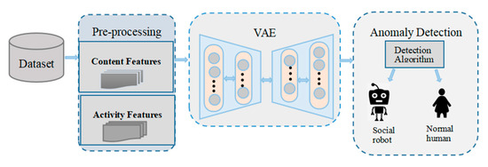
Figure 1.
Social media bot detection framework.
3.2. Feature Extraction
In this paper, the sample dataset is represented as ,, where represents the lth eigenvalue of sample i in the eigenmatrix and l represents the feature dimension of the sample in the feature matrix. In order to describe the human intervention behind social network accounts, the detection model needs to use a variety of features. Features can be classified into five types, including content features, emotional features, account information features, user activity features, and network features [13]. Most of the features selected in studies come from these categories, and all of them are used for classification. According to the characteristics of the selected dataset, this paper extracts several high-usage content features and user activity features. Content features are message-related features, which are obtained through message analysis. User activity characteristics include any measure of how often users post tweets, the similarity between multiple tweets published by users, and how users post tweets (e.g., through mobile devices, web interfaces, or automated tools). In this type of feature, some statistical indicators are calculated according to some or all tweets of users, and the statistical characteristics are expressed as the ratio between the number of times an element appears and the number of tweets. The common features extracted in this paper are as follows.
- (1)
- The average number of mentions in tweets is : social media bots and normal users refer to other users for some special purpose, which leads to different proportions of tweets containing @ in all tweets. The definition of this indicator is as follows:
The meaning of in Equations (1) and (2) is the total number of tweets sent by sample i. is the total number of tweets containing @. The Cumulative Distribution Function (CDF) curve can quantitatively display the distribution of data. Each CDF curve represents the data distribution of a certain feature of a group of samples. Through the CDF curve, we find the differences in the data distribution of statistical characteristics corresponding to multiple sample groups. The cumulative distribution of the average mentions of tweets in the dataset [32] of this paper is shown in Figure 2a. The @ ratio of most social media bots is lower than that of common users, which indicates that social media bots do not have a large number of mentions of other users when they tweet. This is because a large number of @ will cause a poor experience for the tagged accounts, and social media platforms may close such accounts. In order to ensure the long-term validity of the account, social media bots no longer use this method to spread information. On the contrary, real users will have some @ behaviors on the Internet, so this feature can be used as an important indicator to distinguish social media bots from normal users.
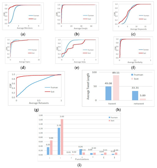
Figure 2.
Feature analysis. (a) The cumulative distribution of the average mentions of tweets (b) The cumulative distribution of the average number of emojis used in tweets (c) The cumulative distribution of stop words (d) The cumulative distribution of topic participation (e) The cumulative distribution of link usage (f) The cumulative distribution corresponding to the proportion of tweet forwarding (g) The cumulative distribution function of the average similarity of tweets (h) Histogram of average length of original and forwarded tweets (i) Histogram of average number of the punctuations (“,”, “.”, “;”, “””, “!”, “(”, and “)”).
- (2)
- The average number of emojis used in tweets is ; the writing style of social media bots is very different from that of normal users. Bots’ tweets are full of emojis or have no facial emojis at all. However, the use of emojis by normal users is not so extreme. This indicator is defined as follows:
is the total number of emojis in tweets. The cumulative distribution of the average number of emojis used in tweets is shown in Figure 2b. The beginning of the two curves shows that the tweets of normal users and social media bots contain fewer emojis, while normal users use a small number. On the contrary, social media bots use the highest number of emojis in 100 tweets, with an average of 68. The average emoji number of normal users is four, so the use of emojis is an important indicator to distinguish social media bots from normal users.
- (3)
- The average number of stop words in tweets is expressed as : stop words are the most frequently used words in tweets, so they represent the writing style of tweet accounts. There are some differences in the use of stop words between normal human users and social media bots, as indicated by the following equation:where is the total number of stop words used in tweets. The cumulative distribution of stop words is shown in Figure 2c. Stop words reflect users’ language habits. Normal human users use stop words more consistently than social media bots. Almost every tweet contains stop words. In the figure, the CDF curve of common users rises steadily, while that of social media bots fluctuates. Thus, stop words are helpful for social media bot detection.
- (4)
- The average number of topics in tweets is expressed as : the #xx form indicates that a specific topic is instantiated on Twitter. Both normal users and social media bots pay attention to certain topics and participate in discussions. Some social media bots participate in a large number of discussions to achieve their goals and improve their reputation. The definition of the average topic tag usage is as follows:where is the total number of stop words used in tweets. The cumulative distribution of topic participation is shown in Figure 2d. Compared with social media bots, the curve of normal users is relatively smooth. However, social media bots participate in few topics at the beginning, and then the number of topics increases sharply. The situation of normal users participating in topics is more stable, because the interests of normal users do not fluctuate too much. It can be seen that the usage of topic tags can be used as a detection indicator.
- (5)
- The average number of links in tweets is expressed as : social media bots always post tweets for some purpose, such as spreading harmful links or advertisements, while social platforms limit the length of tweets and cannot explain all the contents in detail. Therefore, hyperlinks are used to link to other platforms, which leads to a higher proportion of tweets where links are used than normal. The percentage of defined links is as follows:where is the total number of links in tweets. The cumulative distribution of link usage is shown in Figure 2e. From the two curves, we can see that the CDF curve of normal users rises steadily, while the CDF curve of social media bots fluctuates greatly. Moreover, the proportion of links in most normal users’ tweets is lower than that of social media bots. Link reference can be used to distinguish normal users from social media bots.
- (6)
- The proportion of retweets is expressed as : publishing tweets is the main activity in social platforms. Social media bots and normal users generally increase their popularity or participate in activities by retweeting others’ content and continuously publishing original tweets in a certain field. We define the forwarding rate to observe the difference between malicious social media bots and real users. The definition of the forwarding rate is as follows:where is the number of tweets retweeted by users. The cumulative distribution corresponding to the proportion of tweet forwarding is shown in Figure 2f, and the retweet rate distribution of real users is relatively uniform. With the increase in the retweet rate, the curve increases steadily. However, the CDF curve of social media bots fluctuates little at the beginning and stays low, while the forwarding rate rises sharply in the later stage, which indicates that the tweets of social media bots are either not retweeted, or most of them are retweeted, and the retweeted tweets rarely express their own opinions. It can be seen that the retweet rate is a distinguishing feature.
- (7)
- The average similarity of tweets is expressed as : social media bots publish tweets mechanically. Messages belonging to the same social media bots are very similar. Term Frequency Inverse Document Frequency (TF-IDF) is used to weight each word. Then, the cosine similarity is calculated for each pair of tweets. Finally, the average of the obtained scores is taken as the feature. The cumulative distribution function is shown in Figure 2g. The content similarity of most common users is very low, and the curve of social media bots rises sharply after 0.8. The highest similarity of normal users is 17.45%, and the highest similarity of social media bots is 98.2%. This shows that social media bots often send similar tweets, and there may be a situation of batch-publishing identical tweets, so the similarity index of tweets can better distinguish social media bots from normal users.
- (8)
- The average length of original tweets is expressed as : the style of tweets published by normal users and social media bots is not consistent, and the length of relevant tweets is also different, including original tweets and forwarded tweets. As shown in Figure 2h, the average length of tweets sent by normal users and social media bots is counted. On the left side is the average length of a user’s original tweets. The average length of tweets of normal users is much lower than that of social media bots. Social media bots usually add a lot of irrelevant information to their tweets to achieve the purpose of dissemination.
- (9)
- The average length of forwarded tweets is : compared with original tweets, the length of tweets forwarded by social media bots is much shorter than that of normal users, as shown in Figure 2h. It can be seen that social media bots only retweet without making comments.
- (10)
- The average number of the seven kinds of punctuations has seven dimensions: the mathematical expressions of the symbols “,”, “.”, “;”, “””, “!”, “(”, and “)” are, respectively, , , , , , , and . Figure 2i shows the average usage of symbols in tweets by normal users and social media bots. It can be seen from the figure that there are great differences in the usage of symbols in tweets between normal users and social media bots.
3.3. Anomaly Detection
VAE, as a form of a deep generation model, is a generative network structure based on Variable Bayes (VB) inference. The structure is shown in Figure 3. VAE uses two neural networks to establish two probability density distribution models: one is used for variational inference of original input data to generate the variational probability distribution of hidden variables, which is called an inferential network; the other is to restore the approximate probability distribution of the original data according to the generated variational probability distribution of hidden variables, which is called a generative network. The sample set is , where each sample is a randomly generated independent, continuous, or discrete distribution variable. The observable variable X is a random vector in a high-dimensional space, which is used as the input visible layer variable, and then the hidden layer unobservable variable Z is generated. Z is a random vector in a relatively low-dimensional space, and the dataset is generated by a generative network. The VAE generation model includes two processes:
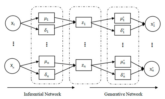
Figure 3.
VAE structure. * represent variables in the Generation Network in Figure.
- (1)
- Approximate the inference process of hidden variable Z posterior distribution: the recognition model , an inferential network, represents the process of inferring z from a known value of x.
- (2)
- Generate the conditional distribution of variables : conditional distribution , namely a generative network.
VAE uses KL divergence to measure the similarity between and true posterior distribution and minimizes KL divergence by optimizing constraint parameters (generative network parameters) and (inferential network parameters).
where argmin is used to minimize KL divergence. is the variational lower bound function of the logarithmic marginal likelihood of the set X, which means we calculate the parameters and according to the known sample set X.
The optimization objective of inferential network and generative network is to maximize the variational lower bound function.
In the above equation, argmax is the function L that maximizes the lower bound of variation. The sampling of Z is as follows:
The latent variable corresponding to sample i is represented as in Equation (10). i means the average value of sample i in the inferential network, and i means the variance of sample i in the inferential network. The mean and variance of the network are derived from the neural network and can be calculated directly. In order to sample Z, an auxiliary parameter is introduced, ε, which is obtained by random sampling from the standard normal distribution N(0,1). represents the randomly sampled data when the hidden layer variable is generated, corresponding to sample i. With this sampling method, the lower bound function is changed to:
With the introduction of auxiliary parameters, the relationship between the hidden variable Z and the mean variance changes from sampling calculation to numerical calculation. The optimization can directly use the Adam or Gradient Descent, and the conditional distribution obeys Bernoulli or Gaussian distribution, which can be calculated directly according to its probability density function formula. Then, each term of the lower bound can be calculated directly; the parameters of all visible and hidden elements will be updated according to the training, the model structure is determined, and the corresponding data can be generated according to the input data.
The original feature matrix and decoded new feature matrix are fused to get the matrix Y . Because the number of abnormal users is lower than that of normal users, and the cost of existing methods is high, combining with the anomaly detection algorithm can not only solve the problem of the imbalance of positive and negative samples but can also improve detection. In the proposed framework, this paper adopts the anomaly detection model based on k-nearest neighbor, and a specific description of the algorithm is given in Algorithm 1. The outlier detection model based on k-nearest neighbor is introduced as follows.
- (1)
- The distance between each sample in the test set and all samples in the training set is calculated once;
- (2)
- The k-nearest distances corresponding to each sample are averaged;
- (3)
- The sample set is sorted in descending order, and the first n (the number of outliers in the test set) points in the sorting table are taken as exception samples.
| Algorithm 1. Specific description of the algorithm. |
| Input: Dataset X; Parameter: and ; Mini-batch: batch; Epochs: epoch; Learning rate: lr. |
| Output: Detection results. |
|
4. Experiments
This section describes the analysis method and data of three groups of experiments.
4.1. Data Description
At present, many scholars are engaged in research on social media bots, and some have collected datasets and published them on the bot repository platform. We selected the author profiling task 2019 (CLEF2019) dataset [32] for this paper, which aims to identify the nature of the Twitter account, detect whether the account is a social media bot or a human, and determine the gender of the account.
The CLEF2019 dataset consists of two groups of Twitter accounts, one in English and the other in Spanish. Each account in the dataset is a collection of 100 tweets. The datasets of different languages are divided into a training set and a test set. Each account is described by two aspects, as shown in Figure 4. The first column defines the nature of the account, and the second column gives the gender. Tweets are not processed to maintain a real scene so that one can know whether a tweet is original or forwarded. The English part of the dataset consists of 4120 accounts, of which 2880 belong to the training set and 1240 belong to the test set. The Spanish part has 3000 users; the training set has 2080 accounts, and the remaining users are the test set. In all the partitions, users are divided into bots and humans, while humans are divided into men and women. The proportion of social bots and human users in all the English datasets was half and half. As shown in Table 1, the length of tweets from different accounts varies greatly: the smallest tweet has only one character, while the longest tweet has more than 900 characters.
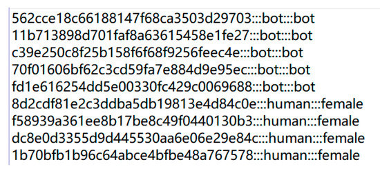
Figure 4.
Account description.

Table 1.
Data description.
The original feature matrix and the decoded new feature matrix are fused to get Y as the input of the anomaly detection part. In order to better describe the overall performance of the model, this paper selects AUC (area under the curve), precision, recall, and training time as evaluation indexes. AUC is the area under the ROC curve (the subject working characteristic curve). True Position Rate indicates the proportion of positive samples successfully identified as positive samples in all samples. False Position Rate indicates the proportion of negative samples successfully identified as positive samples in all samples. The calculation of each index is as follows.
where TP is the number of positive samples determined to be correct, FP is the number of negative samples determined to be positive, FN is the number of positive samples determined to be negative, M is the number of positive samples, and P is the number of negative samples.
4.2. Results and Analysis
In this paper, the features defined in Section 3.2 are extracted, and 16-dimensional normalization processing is used in this part of the experiment. In order to analyze the effectiveness of this method for social media bot detection, the following three groups of experiments are set up.
Experiment 1: This part of the experiment is set up to verify the influence of some parameters on the detection effect. Firstly, the original feature needs to be encoded by the encoder, and the input feature dimension of the encoder is 16. The dimension of the feature is reduced after the encoder. The variational probability distribution of the hidden variables in the VAE will affect the decoding and the subsequent anomaly detection performance. Latent_dim shows the influence of different dimensions on the detection effect, with the number of variables being 2, 4, 6, 8, 10, 14, and 16, respectively. The parameters of the kNN detector take the default value first, where the number of neighbors is 5, and the input is the fusion of decoded features and original features, with a total of 32 dimensions. The influence of different latent_dim values on the detection effect is shown in Figure 5; the final effect is better with the increase in latent_dim. When latent_dim is 16, the hidden variable dimension is equal to the input dimension, and the effect is the best. As shown in Figure 6, the training loss fluctuates with the change in the number of training rounds. When the number of epochs reaches 200, the variational encoder begins to stabilize. Figure 7 shows the encoding and decoding instantiation process of VAE. The input dimension is 16, and the corresponding decoding is also 16.
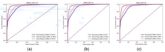
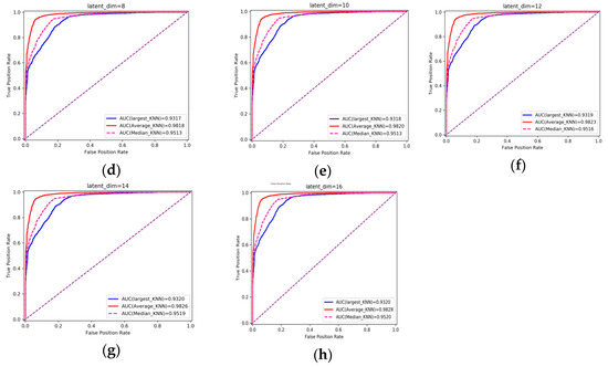
Figure 5.
Influence of different latent_dim on detection effect. (a–h) correspond to AUC obtained when latent_dim is taken as 2, 4, 6, 8, 10, 12, 14 and 16 respectively.
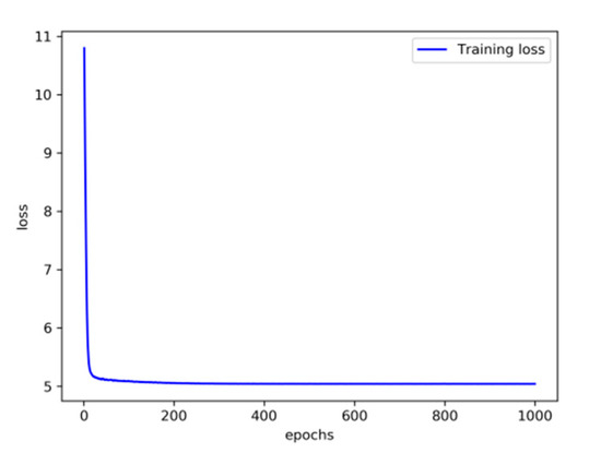
Figure 6.
Training loss fluctuates with the change in the number of training rounds.
Figure 7.
VAE encoding and decoding instantiation process.
The decision rules of kNN include using the distance to the Kth neighbor as the outlier score (largest), using the average of all K neighbors as the outlier score (mean), and using the median of the distance to K neighbors as the outlier score (median). It can be seen from the figure that the effect of the mean is always stronger than the other two rules. The subsequent experiments will choose the mean as the decision rule.
When latent_dim is equal to 16, and the mean and K are chosen to have the default value of 5, AUC = 98.28%. When a smaller value of K is chosen, it is equivalent to using a smaller neighborhood training instance for the prediction, and the approximation error of learning will be reduced. On the contrary, if we choose a larger K value, it is equivalent to using the training instance in a larger neighborhood for prediction to reduce the estimation error. However, the disadvantage is that the approximate error will increase. Too large or too small is not good, so this paper uses cross-validation to select an appropriate K value. Figure 8 shows the different detection effects with the change in K value. It can be seen from the figure that when K is 1 to 6, AUC is increasing. When K is greater than 6, AUC gradually decreases with the increase in K. When K is set to 6, the detection effect is the best, and the AUC is 98.34%.
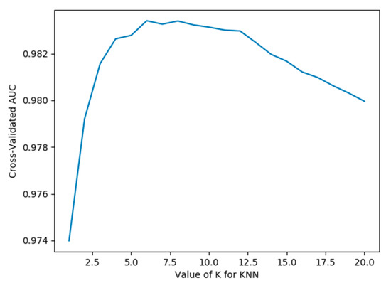
Figure 8.
Influence of different k values on the detection effect.
Experiment 2: To verify the effect of fusion decoding features and original features on detection, in this part, the influence of the original features and fusion features on the detection effect is compared. The VAE-KNN-1 detection method means that the original features are 16 dimensions input to KNN, the VAE-KNN-2 detection method means that the decoded features are 16 dimensions input to KNN, and the VAE-KNN-3 detection method means that the combined features of decoded features and original features are 32 dimensions input to KNN. Table 2 compares the influence of different types of features on the detection effect. It can be seen from the table that, when all indicators are combined, the detection effect will improve, but the fused features will correspondingly increase the feature dimension, resulting in an increase in the training time. In addition, there is a gap between the features after VAE decoding and the original features; the decoded features result in poorer precision.
Table 2.
Compares the effects of different types of features on the detection results.
Experiment 3: To analyze the effectiveness of this framework for social media bot detection, we used eight anomaly detection algorithms as the comparison group. Through the above experiments, we selected the appropriate decoding features and fused the original features as the input of each algorithm in this part. These algorithms are very common in the field of anomaly detection, including the angle-based outlier detector (ABOD) [33], cluster-based local outlier factor (CBLOF), feature bagging, HBOS, IForest, OCSVM, fully connected autoencoder (AE), and VAE. The comparison results of the nine algorithms are shown in Figure 9 and Table 3. The figure and table compare the effects of each anomaly detection algorithm from different indicators. It can be seen from the figure and table that the sensitivity of different detection algorithms to outliers is different from AUC, precision, and time. HBOS performs poorly in AUC and precision evaluation indicators, and VAE based on neural network structure costs a lot in training time. Compared with other algorithms, the results of the proposed method are better, and the training time is shorter, which shows that the overall performance of the proposed algorithm is better.
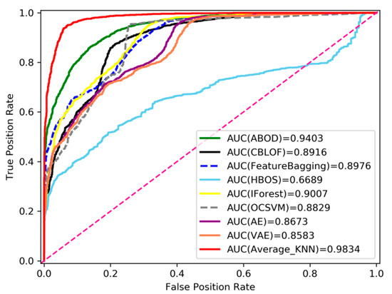
Figure 9.
Comparison of anomaly detection algorithms based on the AUC index.
Table 3.
Comparison of each anomaly detection algorithm based on precision and time index.
5. Conclusions
In this paper, we proposed a new social media bot detection method, using VAE to encode and decode features, and normal data for training. The normal sample features are more similar to the initial features after decoding, while the abnormal samples are different from the initial features. The original features are combined with the decoded features, and then the abnormal algorithm is used for detection. Finally, we conducted some experiments on the public social media bot dataset and analyzed the influence of different parameters, features, and anomaly detection algorithms on social media bot detection through a large number of experiments. The experimental results show that the detection method proposed in this paper effectively improves the corresponding evaluation index results. Therefore, the detection method proposed in this paper is effective. However, there are imperfections to this method, and a series of problems need to be explored, such as the limited feature extraction of the data, how to fuse and extract more distinguishing features to further improve the detection effect, how to adapt to different language environments, and how to identify bot attributes in social media bot detection. There are many social media bot accounts in the social network, so there is still plenty of material to fuel future research work.
Author Contributions
Conceptualization, X.W.; investigation, X.W., Q.Z., K.Z., Y.S. (Yi Sui), and S.C.; methodology, Q.Z. and S.C.; software, Q.Z.; data curation, X.W., Q.Z., Y.S. (Yutong Shi), and Y.S. (Yi Sui); formal analysis, X.W., Q.Z., and Y.S. (Yi Sui).; validation, X.W., K.Z., and Y.S. (Yutong Shi); writing—original draft, X.W., Q.Z., K.Z., Y.S. (Yi Sui), and S.C.; writing—review and editing, X.W., Q.Z., K.Z., Y.S. (Yi Sui), and Y.S. (Yutong Shi). All authors have read and agreed to the published version of the manuscript.
Funding
This research was funded by the National Key R&D Program of China, grant number 2017YFB0802803, and the Beijing Natural Science Foundation, grant number 4202002.
Institutional Review Board Statement
Not applicable.
Informed Consent Statement
Not applicable.
Data Availability Statement
The data set comes from literature (https://link.springer.com/chapter/10.1007/978-3-030-28577-7_30), and If you need data, please ask the authors.
Conflicts of Interest
The authors declare no conflict of interest.
References
- Lee, M.; Oh, S. An Information Recommendation Technique Based on Influence and Activeness of Users in Social Networks. Appl. Sci. 2021, 11, 2530. [Google Scholar] [CrossRef]
- Ferrara, E.; Varol, O.; Davis, C.; Menczer, F.; Flammini, A. The rise of social bots. Commun. ACM 2016, 59, 96–104. [Google Scholar] [CrossRef]
- Howard, P.N.; Woolley, S.; Calo, R. Algorithms, bots, and political communication in the US 2016 election: The challenge of automated political communication for election law and administration. J. Inf. Technol. Politics 2018, 15, 81–93. [Google Scholar] [CrossRef]
- Mesnards, N.; Hunter, D.S.; Hjouji, Z.E.; Zaman, T. The Impact of Bots on Opinions in Social Networks. arXiv 2018, arXiv:1810.12398. [Google Scholar]
- Varol, O.; Ferrara, E.; Davis, C.A.; Menczer, F.; Flammini, A. Online Human-Bot Interactions: Detection, Estimation, and Characterization. arXiv 2017, arXiv:1703.03107v1. [Google Scholar]
- Kingma, D.P.; Welling, M. Auto-Encoding Variational Bayes. arXiv 2014, arXiv:1312.6114. [Google Scholar]
- Lingam, G.; Rout, R.R.; Somayajulu, D. Detection of Social Botnet using a Trust Model based on Spam Content in Twitter Network. In Proceedings of the 2018 IEEE 13th International Conference on Industrial and Information Systems (ICIIS), Rupnagar, India, 1–2 December 2019. [Google Scholar]
- Rout, R.R.; Lingam, G.; Somayajulu, D. Detection of malicious social bots using learning automata with url features in twitter network. IEEE Trans. Comput. Social Syst. 2020, 99, 1–15. [Google Scholar] [CrossRef]
- Zhang, C.; Wu, B. Social Bot Detection Using “Features Fusion”. In Proceedings of the 2020 2nd International Conference on Information Technology and Computer Application (ITCA), Guangzhou, China, 18–20 December 2020; pp. 626–629. [Google Scholar]
- Bacciu, A.; Morgia, L.; Nemmi, E.N.; Neri, V.; Stefa, J. Bot and Gender Detection of Twitter Accounts Using Distortion and LSA; CLEF: Lugano, Switzerland, 2019. [Google Scholar]
- Davis, C.A.; Varol, O.; Ferrara, E.; Flammini, A.; Menczer, F. Botornot: A system to evaluate social bots. In Proceedings of the 25th International Conference Companion on World Wide Web, Montreal, QC, Canada, 11–15 April 2016; pp. 273–274. [Google Scholar]
- Sneha, K.; Emilio, F. Deep neural networks for bot detection. Inf. Sci. 2018, 467, 312–322. [Google Scholar]
- Loyola-Gonzalez, O.; Monroy, R.; Rodriguez, J.; Lopez-Cuevas, A. Contrast Pattern-Based Classification for Bot Detection on Twitter. IEEE Access 2019, 7, 45800–45817. [Google Scholar] [CrossRef]
- Dickerson, J.P.; Kagan, V.; Subrahmanian, V.S. Using sentiment to detect bots on Twitter: Are humans more opinionated than bots? In Proceedings of the 2014 IEEE/ACM International Conference on Advances in Social Networks Analysis and Mining (ASONAM), Beijing, China, 17–20 August 2014; pp. 620–627. [Google Scholar]
- Yang, K.C.; Varol, O.; Davis, C.A.; Ferrara, E.; Flammini, A. Arming the public with artificial intelligence to counter social bots. Hum. Behav. Emerg. Technol. 2019, 1, e115. [Google Scholar] [CrossRef]
- Cai, C.; Li, L.; Zengi, D. Behavior enhanced deep bot detection in social media. In Proceedings of the 2017 IEEE International Conference on Intelligence and Security Informatics (ISI), Beijing, China, 22–24 July 2017; pp. 128–130. [Google Scholar]
- Andrew, H.; Loren, T.; Aaron, H. Bot Detection in Wikidata Using Behavioral and Other Informal Cues. In Proceedings of the ACM on Human-Computer Interaction, New York, NJ, USA, 3–7 November 2018; Volume 2, p. 64. [Google Scholar]
- Qiang, C.; Sirivianos, M.; Yang, X.; Pregueiro, T. Aiding the Detection of Fake Accounts in Large Scale Social Online Services. In Proceedings of the Usenix Conference on Networked Systems Design & Implementation; USENIX Association: Berkeley, CA, USA, 2012. [Google Scholar]
- Wang, G.; Mohanlal, M.; Wilson, C.; Metzger, M.; Zheng, H.; Zhao, B.Y. Social Turing Tests: Crowdsourcing Sybil Detection. arXiv 2012, arXiv:1205.3856. [Google Scholar]
- Nguyen, T.D.; Cao, T.D.; Nguyen, L.G. DGA Botnet detection using Collaborative Filtering and Density-based Clustering. In Proceedings of the Sixth International Symposium ACM, Hue, Vietnam, 3–4 December 2015; pp. 203–209. [Google Scholar]
- Breunig, M.M.; Kriegel, H.P.; Ng, R.T.; Sander, J. LOF: Identifying Density-Based Local Outliers. ACM Sigmod Record 2000, 29, 93–104. [Google Scholar] [CrossRef]
- Liu, F.T.; Ting, K.M.; Zhou, Z.H. Isolation Forest. In Proceedings of the 2008 Eighth IEEE International Conference on Data Mining, Pisa, Italy, 15–19 December 2008. [Google Scholar]
- Ma, J.; Perkins, S. Time-series novelty detection using one-class support vector machines. In Proceedings of the IJCNN’ 03, Portland, OR, USA, 20–24 July 2003; pp. 1741–1745. [Google Scholar]
- Goldstein, M.; Dengel, A. Histogram-based outlier score (hbos): A fast unsupervised anomaly detection algorithm. KI-2012 Poster Demo Track 2012, 24, 59–63. [Google Scholar]
- Lazarevic, A.; Kumar, V. August. Feature bagging for outlier detection. In Proceedings of the KDD ’05, Chicago, IL, USA, 21–24 August 2005. [Google Scholar]
- Shyu, M.L.; Chen, S.; Sarinnapakorn, K.; Chang, L. A novel anomaly detection scheme based on principal component classifier. In Proceedings of the IEEE Foundations and New Directions of Data Mining Workshop, in conjunction with the Third IEEE International Conference on Data Mining (ICDM’03) IEEE, Melbourne, FL, USA, 19 December 2003; pp. 353–365. [Google Scholar]
- Hardin, J.; Rocke, D.M. Outlier detection in the multiple cluster setting using the minimum covariance determinant estimator. Comput. Stat. Data Anal. 2004, 44, 625–638. [Google Scholar] [CrossRef]
- Angiulli, F.; Pizzuti, C. Fast outlier detection in high dimensional spaces. In Proceedings of the European Conference on Principles of Data Mining and Knowledge Discovery; Springer: Berlin/Heidelberg, Germany, 2002; pp. 15–27. [Google Scholar]
- Jeeyung, K.; Alex, S.; Jinoh, K.; Kesheng, W. Botnet Detection Using Recurrent Variational Autoencoder. In Proceedings of the 2020 IEEE Global Communications Conference, Taipei, Taiwan, 7–11 December 2020. [Google Scholar]
- Jia, G.; Liu, G.; Yuan, Z.; Wu, J. An Anomaly Detection Framework Based on Autoencoder and Nearest Neighbor. In Proceedings of the 2018 15th International Conference on Service Systems and Service Management (ICSSSM), Hangzhou, China, 21–22 July 2018. [Google Scholar]
- Jiao, Y.; Rayhana, R.; Bin, J.; Liu, Z.; Kong, X. A steerable pyramid autoencoder based framework for anomaly frame detection of water pipeline CCTV inspection. Measurement 2021, 174, 109020. [Google Scholar] [CrossRef]
- Rangel, F.; Rosso, P. Overview of the 7th Author Profiling Task at PAN 2019: Bots and Gender Profiling. In Proceedings of the CLEF 2019 Labs and Workshops, Notebook Papers, Lugano, Switzerland, 9–12 September 2019. [Google Scholar]
- Kriegel, H.P.; Schubert, M.; Zimek, A. Angle-based outlier detection in high-dimensional data. In Proceedings of the 14th ACM SIGKDD International Conference on Knowledge Discovery and Data Mining, Las Vegas, NV, USA, 24–27 August 2008. [Google Scholar]


Publisher’s Note: MDPI stays neutral with regard to jurisdictional claims in published maps and institutional affiliations. |
© 2021 by the authors. Licensee MDPI, Basel, Switzerland. This article is an open access article distributed under the terms and conditions of the Creative Commons Attribution (CC BY) license (https://creativecommons.org/licenses/by/4.0/).