Topology Optimization Considering Porosity Defects in Metal Additive Manufacturing

Abstract

In this paper, considering the porosity defects of Additive Manufacturing (AM), a level set topology optimization method for AM with porosity constraints is proposed. The concept of topological sensitivity is used to formulate a global porosity constraint function in the proposed method, and a level set topology optimization model considering porosity defects is obtained. To improve the robustness of the algorithm, the topology optimization model is solved in two phases. At first, the classical level set method without the porosity constraint is used to initially optimize the structure. During this process, the hole nucleation method combining bi-directional evolutionary structural optimization (BESO) and the topological sensitivity is used. Secondly, the topology optimization considering the effects of porosity is implemented on the preliminary optimization results. After performing the two-step optimization, a robust structure that alleviates the harmful impact of porosity defects is obtained. Finally, the robustness and effectiveness of the proposed method are validated by several two-dimensional numerical examples.

1. Introduction

Topology optimization is a calculation method that achieves the optimal material configuration in the design domain according to the given boundary conditions and the load conditions. In the past decades, many effective topology optimization methods have been studied and applied, e.g., the homogenization method [1,2,3,4,5], the Solid Isotropic Material with Penalization (SIMP) method [6,7,8,9], the Evolutionary Structural Optimization (ESO) method [10,11,12,13,14], the Moving Morphable Component (MMC) method [15,16,17,18], and the level set method [19,20,21,22,23,24,25]. In particular, the level set method is introduced as an alternative new method in the structural optimization field. This method uses a higher-dimensional level set function to implicitly represent the structural boundary (zero level set) and then obtains the updated structural boundary via the evolution of the level set function during the optimization process. This implicit expression can avoid the relaxation of design variables and numerical instability. As a result, the level set topology optimization is recognized by many researchers.

The studies and applications of numerous optimization methods have made the field of structural optimization to develop rapidly. For example, Calleja-Ochoa et al. [26] established a method of designing and manufacturing micro-structured ultralight components to achieve the goal of lightweight. Topology optimization achieves lightweight structure but results in a more complex structure. Complex structures cannot be manufactured easily by traditional manufacturing processes (turning, milling, casting, etc.). However, the rapidly developing Additive Manufacturing (AM) technology is a forming method in which materials are overlapped layer by layer, which fully eliminates the limitation of geometric complexity. AM makes it possible to manufacture complex structures derived from topology optimization and provides technical support for the application of topology optimization. On the other hand, affected by the cost of AM, how to reduce the consumption of AM has become an urgent problem to be solved. The topology optimization can effectively reduce material consumption under the condition of satisfying structural performance, which provides a solution for reducing the manufacturing cost of AM. In theory, the characteristics and advantages of both topology optimization and AM enable them to complement each other.

AM has unlimited potential, but it does not have unlimited capabilities. Laser AM is based on the technical principles of point-by-point melting, line-by-line scanning, and layer-by-layer accumulating. The metal material undergoes complex thermodynamic behavior under the action of the laser, and the parts are fabricated after the cyclic process of heating, melting, cooling, and solidifying. When affected by many conditions such as laser power, scanning speed, powder materials, and temperature, defects will inevitably occur in the fabricated parts. In recent years, these defects of laser AM have been studied widely [27,28,29,30,31,32,33,34,35].

Porosity is one of the most common defects in laser metal AM. The shape of pores is relatively regular and mostly spherical, and the size is generally small (within 100 µm) [36,37,38,39]. Most of these defects are generated by gas remaining in the molten pool due to excessive or unstable energy input. In the process of material melting and solidifying, the gas in the molten pool does not have sufficient time to escape. Furthermore, the higher the temperature of the molten pool during the melting process, the higher the solubility of the gas in the molten pool. As the molten pool cools, the temperature and the solubility decrease, and the residual gas increases [39].

In the AM process, eliminating or suppressing porosity defects is a challenging problem. Gäumann et al. [40] presented Epitaxial laser metal forming (E-LMF) to effectively reduce porosity defects in AM process. Clijsters et al. [41] designed a real-time molten pool monitoring system which consists of an optical sensor, data processing, reference database, and quality evaluation. In this system, the sensor collects the melt pool information in the form of an optical signal, and then transmits it to the data processing module to establish the melt pool image. Then, the location and size of the defects are determined by comparing with the reference database. Finally, the process parameters are optimized by the feedback system to reduce the porosity. Although the proposed methods can effectively reduce the porosity defects, they cannot completely remove the porosity defects.

It is well known that stress concentration occurs near the defects of the fabricated part. Under the external load, the stress near the defects will increase significantly. When the ultimate strength of the material is exceeded, cracks are generated and gradually expand until fracture failure. Thus, the existence of porosity has a significant impact on the mechanical properties of the fabricated parts. Moreover, the pores not only are the source of fatigue cracks but also accelerate the expansion of fatigue cracks under the stress concentration, greatly reducing the fatigue life of the fabricated part. The more pores in the fabricated parts, the more cracks may occur. It is difficult to satisfy the requirements with the existence of porosity, which restricts the usability of the fabricated parts.

According to our investigation, few researchers consider the porosity defects of the AM in the topology optimization problem. In this paper, the concept of topological sensitivity is employed to construct a porosity constraint function in the form of domain integral and a level set topology optimization model considering the effects of porosity is proposed. To improve the robustness of the algorithm, the topology optimization model is solved by two steps. At first, the classical level set method is used to initially optimize the structure. Secondly, the porosity is taken into topology optimization of the structure after the initial optimization, and a robust structure that minimizes the impact of porosity is obtained.

Since the reinitialization retains the properties of the signed distance function, the holes cannot be automatically nucleated in the solid design domain, i.e., the topology change can only rely on the existing initial structural boundary. In the past few decades, some solutions have been proposed for hole nucleation. Allaire et al. [42] proposed a level set topology optimization method that inserts holes according to the value of topological sensitivity. He et al. [43] added topological sensitivity as a diffusive term of the Hamilton–Jacobi equation, so that new holes were automatically nucleated during the optimization process. Xia et al. [44] proposed a hole nucleation method in combination with bi-directional evolutionary structural optimization (BESO) based on the material removal scheme. Yaghmaei et al. [45] proposed a filtering level set method to nucleate holes and avoid re-initialization of level set function. Although the above hole nucleation method makes the level set method unnecessary to guess the initial structure, the effect of hole nucleation is not ideal for various reasons. Therefore, it is necessary to propose a new hole nucleation method.

In the present work, a new level set hole nucleation method is proposed by combining the BESO method with topological sensitivity. This method can automatically find and nucleate holes within the design domain.

The rest of this paper is organized as follows: Section 2 reviews the level set topology optimization methods. Section 3 describes the hole nucleation method combining BESO and topological sensitivity. In Section 4, a level set topology optimization model considering porosity defects is formulated, and the shape sensitivity of the constraint function is calculated. Section 5 lists the optimization procedure. Section 6 gives numerical examples and discussions. Finally, the paper is summarized in Section 7.

2. Level Set Topology Optimization

In the level set topology optimization of continuum structure, an optimal design Ω is sought in the design domain D, and ∂Ω is the boundary of Ω. The topology of the structure is described by the implicit level set function Φ(x) as:

$$\{\begin{array}{l}\Phi \left(x\right)>0 x\in \mathsf{\Omega }\\ \Phi \left(x\right)=0 x\in \partial \mathsf{\Omega }\\ \Phi \left(x\right)<0 x\in D{\displaystyle \cap }\overline{\mathsf{\Omega }}\end{array}$$

(1)

In the problem of maximizing structural stiffness (i.e., minimizing compliance), it is assumed that the constraint condition is the optimized structural volume, and the optimization objective is the compliance. When the load and boundary conditions are given, the topology optimization problem can be described as:

$$\begin{array}{c}\min J\left(u\right)={{\displaystyle \int }}_{\mathsf{\Omega }}f\left(u\right)dx={{\displaystyle \int }}_{\mathsf{\Omega }}Eϵ\left(u\right)·ϵ\left(v\right)dx\\ s.t. {{\displaystyle \int }}_{\mathsf{\Omega }}Eϵ\left(u\right)·ϵ\left(v\right)dx={{\displaystyle \int }}_{\mathsf{\Omega }}Pvdx+{{\displaystyle \int }}_{\partial \mathsf{\Omega }}\tau vds\\ \forall v\in U u{|}_{{\Gamma }_D}=u_0 \\ {{\displaystyle \int }}_{\mathsf{\Omega }}d\mathsf{\Omega }=V_{max} \end{array}$$

(2)

where u is the displacement field, E is the elasticity tensor of the material,$ϵ$ is the strain tensor, P is the body force, τ is the boundary force, ${{\displaystyle \int }}_{\mathsf{\Omega }}^{}d\mathsf{\Omega }$ is the volume of the structure, and V_max is the maximum admissible volume.

This paper aims to study the topology optimization problem of the linear elastic structure, so the boundary ∂Ω of the design domain Ω consists of three parts:

$$\partial \mathsf{\Omega }={\Gamma }_0+{\Gamma }_N+{\Gamma }_D$$

(3)

where Γ_D is the Dirichlet boundary conditions and Γ_N is the Neumann boundary conditions. Therefore, the linear elastic problem described in (2) is also expressed as:

$$\{\begin{array}{l}-div\left(Eϵ\left(u\right)\right)=P \mathsf{\Omega }\\ u=0 {\Gamma }_D\\ \begin{array}{c}\left(Eϵ\left(u\right)\right)n=\tau {\Gamma }_N\\ \left(Eϵ\left(u\right)\right)n=0 {\Gamma }_0\end{array}\end{array}$$

(4)

Then, the objective function based on compliance can be expressed as:

$${{\displaystyle \int }}_{\mathsf{\Omega }}^{}Eϵ\left(u\right)·ϵ\left(u\right)dx={{\displaystyle \int }}_{\mathsf{\Omega }}^{}P·udx+{{\displaystyle \int }}_{{\Gamma }_N}\tau ·uds$$

(5)

Employing the level set function Φ(x), the level set topology optimization problem is written as follows:

$$\begin{array}{c}\min J\left(u,\Phi \right)={{\displaystyle \int }}_{\mathsf{\Omega }}f\left(u\right)H\left(\Phi \right)dx={{\displaystyle \int }}_{\mathsf{\Omega }}Eϵ\left(u\right)·ϵ\left(u\right)H\left(\Phi \right)dx\\ s.t. a\left(u,v,\Phi \right)=L\left(v,\Phi \right) \\ \forall v\in U u{|}_{{\Gamma }_D}=u_0 \\ V\left(\Phi \right)=V_{max} \end{array}$$

(6)

where a(u, v, Φ), L(v, Φ) and V(Φ) are expressed as:

$$\begin{array}{c}a\left(u,v,\Phi \right)={{\displaystyle \int }}_{\mathsf{\Omega }}^{}Eϵ\left(u\right)·ϵ\left(v\right)H\left(\Phi \right)dx\\ L\left(v,\Phi \right)={{\displaystyle \int }}_{\mathsf{\Omega }}^{}PvH\left(\Phi \right)dx+{{\displaystyle \int }}_{\partial \mathsf{\Omega }}\tau v\delta \left(\Phi \right)\left|\nabla \Phi \right|ds\\ V\left(\Phi \right)={{\displaystyle \int }}_{\mathsf{\Omega }}^{}H\left(\Phi \right)dx\end{array}$$

(7)

where H(⋅)is the Heaviside function, which is defined as:

$$H\left(x\right)=\{\begin{array}{c}1 x\ge 0\\ 0 x<0\end{array}$$

(8)

δ(⋅) is the Dirichlet function, and its relationship with the Heaviside function is as follows:

$$\delta \left(x\right)=\frac{dH\left(x\right)}{dx}$$

(9)

To solve the Hamilton–Jacobi partial differential equation, the concept of shape sensitivity is introduced to calculate the velocity field V_n of the level set function. The Murat and Simon analysis [46] based on the Hadamard variational method was used to calculate shape sensitivity. Considering a smooth initial shape Ω₀, all admissible shapes Ω are obtained by applying a smooth vector field θ:

$$\mathsf{\Omega }=\left\{x+\theta \left(x\right), xϵ{\mathsf{\Omega }}_0\right\}$$

(10)

The above equation shows that all admissible shapes are represented by a vector $\theta$, so (10) is also written as:

$$\mathsf{\Omega }=\left(Id+\theta \right)\left({\mathsf{\Omega }}_0\right)$$

(11)

where (Id + θ) is the diffeomorphic mapping of Ω₀.

Then, the shape sensitivity can be defined by the derivative with respect to θ. The shape expression (10) means that all admissible shapes will have the same topology as the initial shape Ω₀. Therefore, the topology cannot be changed by continuously transforming the initial shape Ω₀, which theoretically answers the reason why the level set topology optimization method cannot automatically nucleate holes.

Based on the above assumptions, the shape sensitivity of the objective J(Ω) on Ω₀ can be defined as the Fréchet derivative at θ = 0:

$$J\left(\left(Id+\theta \right)\left({\mathsf{\Omega }}_0\right)\right)=J\left({\mathsf{\Omega }}_0\right)+J^{\prime }\left({\mathsf{\Omega }}_0\right)\left(\theta \right)+o\left(\theta \right), \mathrm{where}\underset{\theta \to 0}{\lim }\frac{\left|o\left(\theta \right)\right|}{\theta }=0$$

(12)

where J(Ω) has first-order continuous differentiability at θ = 0. According to the definition of shape sensitivity, shape sensitivity (12) is also rewritten as:

$$J^{\prime }\left({\mathsf{\Omega }}_0\right)\left(\theta \right)=\underset{\theta \to 0}{\lim }\frac{J\left(\left(Id+\theta \right)\left({\mathsf{\Omega }}_0\right)\right)-J\left({\mathsf{\Omega }}_0\right)}{\theta }$$

(13)

Wang and Allaire have already calculated the shape sensitivity of the optimization problem (6). This paper will directly quote the results, and the detailed process is in Wang and Allaire et al. [19,25].

Lemma 1.

The shape sensitivity of the compliance is:

$$\begin{array}{c}{J}^{\prime }\left(\mathsf{\Omega }\right)\left(\theta \right)={{\displaystyle \int }}_{{\Gamma }_N}\left(2\left[\frac{\partial \left(\tau ·u\right)}{\partial n}+H\tau ·u+Pu\right]-Eϵ\left(u\right)·ϵ\left(u\right)\right)\theta ·nds\\ +{{\displaystyle \int }}_{{\Gamma }_D}\left(Eϵ\left(u\right)·ϵ\left(u\right)\right)\theta ·nds \end{array}$$

(14)

Lemma 2.

The shape sensitivity of the volume constraint is:

$$V^{\prime }\left(\Phi \right)\left(\theta \right)={{\displaystyle \int }}_{\partial \mathsf{\Omega }}\theta \left(x\right)·n\left(x\right)ds$$

(15)

3. Hole Nucleation Method

3.1. BESO

BESO is developed from ESO which was originally proposed by Xie et al. [13] in 1992. ESO allows only to remove material from the structure, and those removed materials cannot be admitted in the later evolutions. Therefore, some elements with higher utilization are accidentally removed. Correspondingly, Xie et al. [14] proposed the BESO that can remove low-efficiency materials and add materials at key positions. This method is widely used in machinery, civil engineering, aerospace, and other fields because of its simple algorithm and easy programming.

In BESO, the sensitivity number is used to remove low-efficiency materials or add high-efficiency materials. In other words, material is removed or added in the design domain by comparing the value of the sensitivity number. Therefore, BESO regards the structure itself as the design variable of the optimization problem. The optimization problem is expressed as:

$$\begin{array}{c}\min C={\mathit{F}}^T\mathit{u}={\mathit{u}}^T\mathit{K}\mathit{u} \\ \begin{array}{c}s.t. {\displaystyle {\displaystyle \sum }_{i=1}^N}{V}_i{x}_i=f{V}^{*}=V_{max}\\ \mathit{F}=\mathit{K}\mathit{u} \end{array}\\ x_i=\{\begin{array}{c}0\\ 1\end{array} \end{array}$$

(16)

where compliance C is the objective of the optimization problem, F is the load vectors, u is the displacement vectors, K is the global stiffness matrix, V_i is the elemental volume, V^* is the total volume of the design domain, f is the volume fraction, and N is the number of elements in the design domain. The design variable x_i is the elemental density with x_i = 0 for a void element and x_i = 1 for a solid element.

In BESO, the sensitivity number is compared with the sensitivity threshold. For solid elements, the sensitivity number is greater than or equal to the threshold. For void elements, the sensitivity number is less than the threshold. The elemental sensitivity number is defined as the change of the mean compliance or elemental strain energy:

$${\alpha }_i^e=\frac{{\mathit{u}}_i^T{\mathit{K}}_i{\mathit{u}}_i}{V_i}$$

(17)

To calculate the sensitivity of void elements, a sensitivity filter scheme is introduced. Furthermore, this filter method can solve the checkerboard and mesh dependency. The formula for sensitivity filter scheme is written as:

$${\alpha }_i=\frac{{{\displaystyle \sum }}_{j\in N_i}\omega \left(r_{ij}\right){\alpha }_j^n}{{{\displaystyle \sum }}_{j\in N_e}\omega \left(r_{ij}\right)}$$

(18)

where α_i is the elemental sensitivity after filtering, and ${\alpha }_j^n$ is the elemental sensitivity before filtering. The neighbor elements set N_i of the element i is defined as all elements whose spatial distance from the central cell i is less than or equal to the filtering radius R_min. The weight factor ω(r_ij) of the spatial distance is:

$$\omega \left(r_{ij}\right)=R_{min}-r_{ij}$$

(19)

where r_ij is the spatial distance between element j and central element i, defined as ||x_j-x_i||.

The sensitivity threshold α^th can be determined by the target volume V^k+1. The target volume can be calculated by the current volume and the evolutionary volume ratio c_er:

$$V^{k+1}=V^k\left(1\pm c_{er}\right)$$

(20)

If the current structure volume is equal to the volume constraint, the target volume V^k+1 will remain V_max.

The finite element analysis, sensitivity filtering, and structure update are continuously looped until the volume constraint and the convergence criterion (21) are satisfied.

$$e=\frac{\left|{{\displaystyle \sum }}_i^N{C}_{k-i+1}-{{\displaystyle \sum }}_i^N{C}_{k-N-i+1}\right|}{{{\displaystyle \sum }}_i^N{C}_{k-i+1}}\le \delta$$

(21)

where e is the change of objective, δ is the tolerance factor, and N is a positive integer.

3.2. Topological Sensitivity

The topological sensitivity defines the impact on the objective when a small hole is inserted at a certain position in the design domain. The topological sensitivity of the objective J(Ω) in a given design domain is defined as:

$$D_T\left(\mathit{x}\right)=\underset{r\to 0}{\lim }\frac{J\left({\mathsf{\Omega }}_r\right)-J\left(\mathsf{\Omega }\right)}{M\left(r\right)}$$

(22)

where M(r) is the measure of the hole B_r. According to reference [47], this paper takes the Lebesgue measure, which can be written as:

$$\underset{r\to 0}{\lim }M\left(r\right)=0$$

(23)

According to the topological-shape sensitivity method [47], topological sensitivity can be solved by shape sensitivity. The relationship between shape sensitivity and topological sensitivity is expressed as:

$$D_T\left(\mathit{x}\right)=D_T^{*}\left(\mathit{x}\right)=\underset{r\to 0}{\lim }\frac{1}{M^{\prime }\left(r\right)\left|V_N\right|}{\frac{dJ\left(\mathsf{\Omega }\right)}{d\theta }|}_{\theta =0}$$

(24)

This paper aims to study the topology optimization problem based on the compliance, so it is necessary to solve the topological sensitivity of the compliance. According to the research of Novotny et al. [48], the topological sensitivity of compliance is:

• for d = 2

  $$D_{T}J\left(\mathit{x}\right)=\frac{\pi \left(\lambda +2\mu \right)}{2\mu \left(\lambda +\mu \right)}\left(4\mu Eϵ\left(u\right)·ϵ\left(u\right)+\left(\lambda -\mu \right)tr\left(Eϵ\left(u\right)\right)tr\left(ϵ\left(u\right)\right)\right)\left(x\right)$$

  (25)
• for d = 3

  $$D_{T}J\left(\mathit{x}\right)=\frac{\pi \left(\lambda +2\mu \right)}{\mu \left(9\lambda +14\mu \right)}\left(20\mu Eϵ\left(u\right)·ϵ\left(u\right)+\left(3\lambda -2\mu \right)tr\left(Eϵ\left(u\right)\right)tr\left(ϵ\left(u\right)\right)\right)\left(x\right)$$

  (26)

  where λ and μ are the Lamé moduli of the material, which satisfy:

  $$\lambda =\frac{E\nu }{1-{\nu }^2}$$

  (27)

  $$\mu =\frac{E}{2\left(1+\nu \right)}$$

  (28)

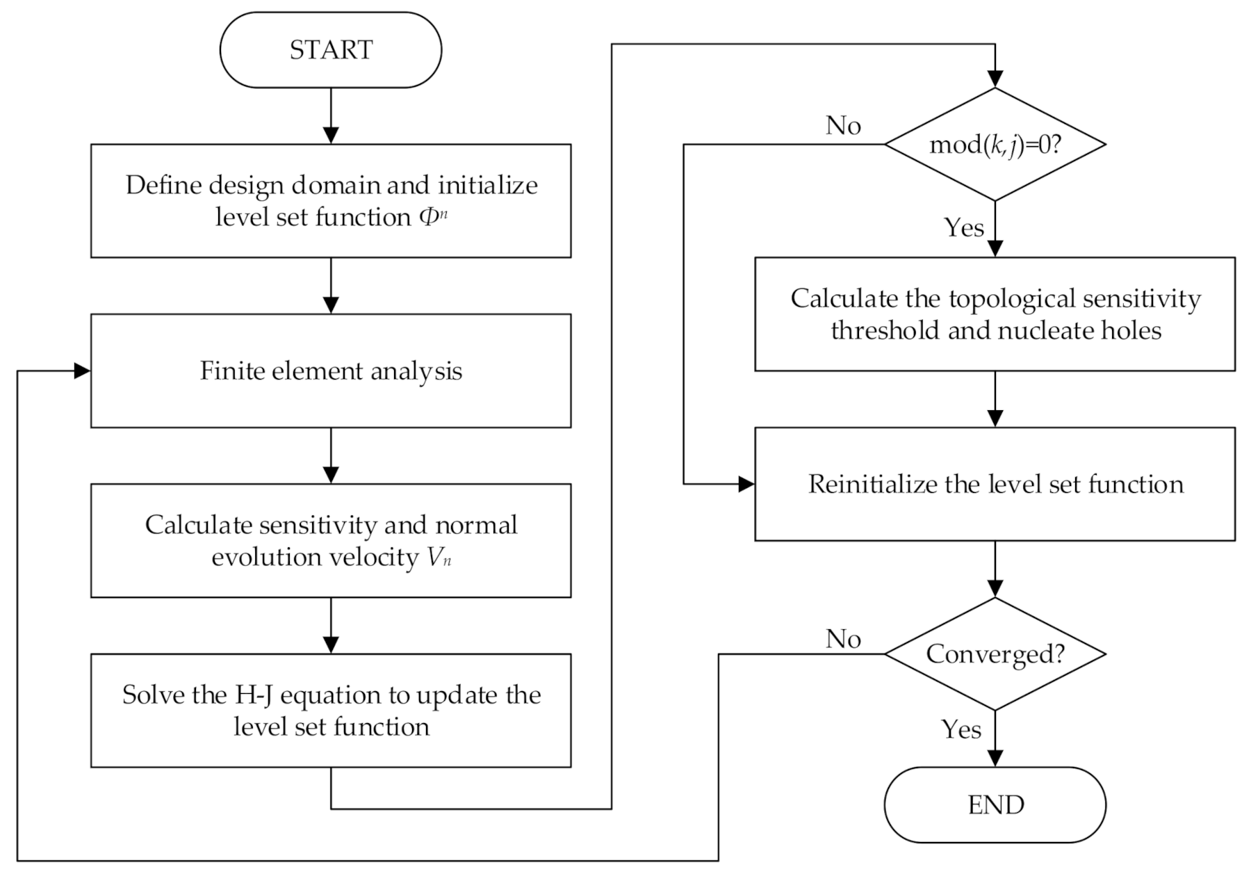
3.3. Hole Nucleation Method Combining BESO and Topological Sensitivities

The BESO method uses the sensitivity number as the criterion to remove low-efficiency materials or add high-efficiency materials to optimize the structure. The topological sensitivity describe the impact of inserting holes on the objective. Using topological sensitivity as the criterion for removing or adding materials in the BESO method has practical physical meaning. Therefore, the combination of BESO and topological sensitivity can be used as a hole nucleation method for level set topology optimization.

Thus, the sensitivity number α_i of BESO can be replaced with the topological sensitivity:

$$D_T^i=\underset{r\to 0}{\lim }\frac{1}{M^{\prime }\left(r\right)\left|V_N\right|}{\frac{dJ\left(\mathsf{\Omega }\right)}{d\theta }|}_{\theta =0}$$

(29)

According to the idea of BESO, adding and removing materials in the current structure requires topological sensitivity threshold $D_T{}^{th}$. The threshold is usually determined according to a given evolutionary volume ratio. Assuming that there are N elements in the design domain, the topological sensitivity $D_T^i$ of all elements is arranged according to the value, that is $D_T^1<D_T^2<\cdots <D_T^V<\cdots <D_T^N$. According to (20), V elements are required to maintain holes (i.e., N-V solid elements), then the topological sensitivity threshold is:

$$D_T{}_1^{th}=D_T^V$$

(30)

However, only using the threshold as in (30) is likely to cause unstable optimization. As the BESO method always needs to add or remove materials, it will continue to add or remove materials from the boundary of the structure when the structure is close to the optimization result. In this case, the boundary based on the evolution of the level set method will continue to be updated, and the material will be added at the position where the material was removed by the BESO method, which will easily cause numerical instability and lead to optimization failure. Therefore, another topological sensitivity threshold $D_T{}_2^{th}$ needs to be introduced in the optimization, and its value is determined according to the average topological sensitivity of the structure boundary ∂Ω. The boundary threshold $D_T{}_2^{th}$ can be described as:

$$D_T{}_2^{th}=\beta \overline{D_T}$$

(31)

where 0 < β < 1 is a user-defined threshold factor, and $\overline{D_T}$ is the average topological sensitivity of the structure boundary ∂Ω.

Therefore, the topological sensitivity threshold of adding and removing materials $D_T{}^{th}$ can be defined as:

$$D_T{}^{th}=\min \left(D_T{}_1^{th},D_T{}_2^{th}\right)$$

(32)

The holes are nucleated every j iteration in this hole nucleation method. After multiple iterations, if the topological sensitivity in the solid domain is greater than or equal to the threshold $D_T{}^{th}$, the hole nucleation process ends.

The procedures of level set topology optimization combining BESO and topological sensitivity are as follows:

• Define the design domain and initialize level set function;
• Solve linear elasticity equation via the Finite Element Method;
• Calculate shape sensitivity, topological sensitivity, and the normal evolution velocity $V_n$;
• Solve the Hamilton–Jacobi equation to update the level set function;
• If the current iteration number is an integer multiple of j, nucleate hole by (45), then go to step 6. Otherwise, go to step 7;
• Calculate the topological sensitivity threshold $D_T{}^{th}$;
• Reinitialize the level set function;
• Check whether the convergence criteria are satisfied. If not, repeat steps 2–8 until convergence.

The flowchart of level set topology optimization combining BESO and topological sensitivity is shown in Figure 1.

4. Constraint Function Considering Porosity Defects

Topology optimization is to find the optimal material distribution to achieve the best structural performance. However, the appearance of porosity in the subsequent AM process will affect the performance of the structure, causing the manufactured parts to fail to satisfy the performance requirements. Therefore, it is necessary to consider the effects of porosity during the structural topology optimization, so that the manufactured parts still satisfy the requirements.

In actual production, the generation of porosity is closely related to laser power, forming speed, scanning scheme, forming environment, and other factors in additive manufacturing. Our method cannot avoid the generation of porosity during the manufacturing process, that is, porosity will still be generated in the optimization results. However, we can consider these porosity defects in the optimization process, so as to reduce its effects on the structural performance of the optimization results. In other words, the optimization results without considering the porosity constraints cannot meet the actual working conditions due to the existence of porosity, while the optimization results considering the porosity constraints can still meet. Therefore, this method can greatly promote the combination of additive manufacturing and topology optimization, so as to greatly improve the production efficiency and capacity.

Topological sensitivity is defined as the impact of objective when a small hole is inserted, which is compatible with the impact of porosity on structural performance. Therefore, this paper will use topological sensitivity to define the porosity constraint function.

4.1. Formulation of Porosity Constraints

Assuming B_x,r = x + rB, x∈Ω represents a small pore with radius r at x in the design domain Ω, the design domain where the pore appears can be expressed as Ω_0,x,r = Ω₀ − B_x,r. The objective function J(Ω₀) does not change significantly due to the appearance of pores in the design domain Ω₀, so the change of structural performance before and after the appearance of pores can be expressed as:

$$c_0=J\left({\mathsf{\Omega }}_{0,x,r}\right)-J\left({\mathsf{\Omega }}_0\right)$$

(33)

Introduce the definition of topological sensitivity in Section 3.2:

$$J\left({\mathsf{\Omega }}_{0,x,r}\right)=J\left({\mathsf{\Omega }}_0\right)+D_{T}J\left({\mathsf{\Omega }}_{0,x,r}\right)M\left(B_{x,r}\right)+o\left(M\left(B_{x,r}\right)\right)$$

(34)

where M(B_x,r) is the measure of the pore B_x,r and $\underset{r\to 0}{\lim }\frac{\left|o\left(M\left(B_{x,r}\right)\right)\right|}{M\left(B_{x,r}\right)}=0$.

By substituting (34) into (33), the result is:

$$c_0=D_{T}J\left({\mathsf{\Omega }}_{0,x,r}\right)M\left(B_{x,r}\right)+o\left(M\left(B_{x,r}\right)\right)$$

(35)

After considering the porosity constraints, assuming that ${\mathsf{\Omega }}_p$ is set as the structural design domain of the optimal design, and J( ${\mathsf{\Omega }}_p$) is the corresponding objective function to characterize the structural performance, the change of structural performance can be obtained:

$$c_p=J\left({\mathsf{\Omega }}_{p,x,r}\right)-J\left({\mathsf{\Omega }}_p\right)=D_{T}J\left({\mathsf{\Omega }}_{p,x,r}\right)M\left(B_{x,r}\right)+o\left(M\left(B_{x,r}\right)\right)$$

(36)

According to the above analysis, the structural performance will decrease after considering the porosity constraint, so the inequality can be established:

$$c_p-\eta c_0\le 0$$

(37)

where η$\in \left(0,1\right]$ is a user-defined tolerance that indicates the admissible change of objective.

In level set topology optimization, the inequality is not conducive to solving by Lagrange method, so inequalities need to be transformed. According to the work of Allaire et al. [49,50], assuming [F]⁺ ≡ max(F, 0), the inequality (37) satisfies:

$${\left[c_p-\eta c_0\right]}_{+}\equiv 0$$

(38)

Equation (38) are constraints defined at various points in the design domain. This type of constraint is inconvenient for implementation in topology optimization and to solve shape sensitivity. Addressing the issue, the domain integral is established:

$${{\displaystyle \int }}_{\mathsf{\Omega }}^{}{\left({\left[c_p-\eta c_0\right]}_{+}\right)}^{2}dx=0$$

(39)

Therefore, the topology optimization problem considering porosity constraints is expressed as:

$$\begin{array}{c}\min J\left(u\right)={{\displaystyle \int }}_{\mathsf{\Omega }}^{}f\left(u\right)d\mathsf{\Omega }={{\displaystyle \int }}_{\mathsf{\Omega }}Eϵ\left(u\right)·ϵ\left(u\right)d\mathsf{\Omega }\\ s.t. {{\displaystyle \int }}_{\mathsf{\Omega }}d\mathsf{\Omega }=V_{max} \\ C_p\left(\mathsf{\Omega }\right)=\frac{1}{2}{{\displaystyle \int }}_{\mathsf{\Omega }}{\left({\left[c_p-\eta c_0\right]}_{+}\right)}^{2}dx=0\end{array}$$

(40)

4.2. Shape Sensitivities of Porosity Constraints

The level set method topology optimization needs to solve the shape sensitivity of the objective and the constraint function. The shape sensitivity of the compliance and the volume constraint have been obtained in Section 2. Next, the shape sensitivity of the porosity constraint function will be derived.

The shape sensitivity of the constraint function is solved by the Céa method. Introducing Augmented Lagrangian:

$$\begin{array}{c}L\left(\mathsf{\Omega },u,p\right)=\frac{1}{2}{{\displaystyle \int }}_{\mathsf{\Omega }}^{}{\left({\left[c_p-\eta c_0\right]}_{+}\right)}^{2}dx+{{\displaystyle \int }}_{\mathsf{\Omega }}^{}Eϵ\left(u\right):ϵ\left(p\right)dx\\ -{{\displaystyle \int }}_{\mathsf{\Omega }}^{}f·pdx-{{\displaystyle \int }}_{{\Gamma }_N}g·pds \end{array}$$

(41)

Under the optimization theory, the stagnation point of the Lagrangian is the optimality condition of the minimization problem. Therefore, the optimal value of the function can be solved by finding the stagnation point of the function. For a given Ω, (u_Ω, p_Ω) represents the stagnation point. At first, take the partial derivative of L(Ω, u, p) with respect to p:

$$\frac{\partial L}{\partial p}\left(\mathsf{\Omega },u,p\right)={{\displaystyle \int }}_{\mathsf{\Omega }}^{}Eϵ\left(u\right):ϵ\left(\widehat{p}\right)dx-{{\displaystyle \int }}_{\mathsf{\Omega }}^{}f·\widehat{p}dx-{{\displaystyle \int }}_{{\Gamma }_N}g·\widehat{p}ds$$

(42)

Let (42) be equal to 0, which is the same as the linear elastic equation in the optimization problem. Therefore, the solution of (42) is equal to the solution of the linear elastic equation, i.e., u = u_Ω = u_e.

Secondly, take the partial derivative of L(Ω, u, p) with respect to u:

$$\frac{\partial L}{\partial u}\left(\mathsf{\Omega },u,p\right)={{\displaystyle \int }}_{\mathsf{\Omega }}^{}{\left[c_p-\eta c_0\right]}_{+}M\left(B_{x,r}\right)D_T^{\prime }J\left(\mathsf{\Omega }\right)\left(\widehat{u}\right)dx+{{\displaystyle \int }}_{\mathsf{\Omega }}^{}Eϵ\left(p\right):ϵ\left(\widehat{u}\right)dx$$

(43)

Let (43) be equal to 0, suppose its solution is p = p_Ω, which results in:

$${{\displaystyle \int }}_{\mathsf{\Omega }}^{}{\left[c_p-\eta c_0\right]}_{+}M\left(B_{x,r}\right)D_T^{\prime }J\left(\mathsf{\Omega }\right)\left(v\right)dx+{{\displaystyle \int }}_{\mathsf{\Omega }}^{}Eϵ\left(p_{\mathsf{\Omega }}\right):ϵ\left(v\right)dx=0$$

(44)

The shape sensitivity of the constraint function can be obtained by differentiating $C_p$(Ω) = L(Ω, u, p). According to the chain derivation rule, the shape sensitivity of the objective function can be obtained as:

$$C_p^{\prime }\left(\mathsf{\Omega }\right)\left(\theta \right)=\frac{\partial L}{\partial \mathsf{\Omega }}\left(\mathsf{\Omega },u,p\right)\left(\theta \right)+\frac{\partial L}{\partial u}\left(\mathsf{\Omega },u,p\right)\left(u^{\prime }\left(\theta \right)\right)$$

(45)

Substituting (u_Ω, p_Ω) into (45), the second term $\frac{\partial L}{\partial u}\left(\mathsf{\Omega },u_{\mathsf{\Omega }},p_{\mathsf{\Omega }}\right)$ on the right side of (45) is equal to 0, so the shape sensitivity of the constraint function is:

$$C_p^{\prime }\left(\mathsf{\Omega }\right)\left(\theta \right)=\frac{\partial L}{\partial \mathsf{\Omega }}\left(\mathsf{\Omega },u_{\mathsf{\Omega }},p_{\mathsf{\Omega }}\right)\left(\theta \right)$$

(46)

Quoting Lemma 4 and Lemma 5 in [20], the result is:

$$\begin{array}{c}\frac{\partial L}{\partial \mathsf{\Omega }}\left(\mathsf{\Omega },u_{\mathsf{\Omega }},p_{\mathsf{\Omega }}\right)\left(\theta \right)=\frac{1}{2}{{\displaystyle \int }}_{\mathsf{\Omega }}^{}{\left({\left[c_p-\eta c_0\right]}_{+}\right)}^2\theta ·nds\\ +{{\displaystyle \int }}_{\mathsf{\Omega }}^{}\left({\left[c_p-\eta c_0\right]}_{+}\right)M\left(B_{x,r}\right)D_T^{\prime }J\left(\mathsf{\Omega }\right)ds\\ +{{\displaystyle \int }}_{\mathsf{\Omega }}^{}Eϵ\left(u_{\mathsf{\Omega }}\right):ϵ\left(p_{\mathsf{\Omega }}\right)\theta ·nds-{{\displaystyle \int }}_{\mathsf{\Omega }}^{}f·p_{\mathsf{\Omega }}·\theta ·nds\\ -{{\displaystyle \int }}_{{\Gamma }_N}g·p_{\mathsf{\Omega }}·\theta ·nds \end{array}$$

(47)

when u∈Γ_N, θ = 0. The shape sensitivity of the constraint function is:

$$\begin{array}{c}{C}_p^{\prime }\left(\mathsf{\Omega }\right)\left(\theta \right)=\frac{1}{2}{{\displaystyle \int }}_{\mathsf{\Omega }}{\left({\left[D_{T}J\left(\mathsf{\Omega }\right)-{\eta }_{B}J\left(\mathsf{\Omega }\right)\right]}_{+}\right)}^2\theta ·nds\\ +{{\displaystyle \int }}_{\mathsf{\Omega }}\left({\left[c_p-\eta c_0\right]}_{+}\right)M\left(B_{x,r}\right)D_T^{\prime }J\left(\mathsf{\Omega }\right)ds\\ +{{\displaystyle \int }}_{\mathsf{\Omega }}\left(Eϵ\left(u_{\mathsf{\Omega }}\right):ϵ\left(p_{\mathsf{\Omega }}\right)-f·p_{\mathsf{\Omega }}\right)\theta ·nds\end{array}$$

(48)

where $p_{\mathsf{\Omega }}$ satisfies:

$${{\displaystyle \int }}_{\mathsf{\Omega }}^{}{\left[c_p-\eta c_0\right]}_{+}M\left(B_{x,r}\right)D_T^{\prime }J\left(\mathsf{\Omega }\right)\left(v\right)dx+{{\displaystyle \int }}_{\mathsf{\Omega }}^{}Eϵ\left(p_{\mathsf{\Omega }}\right):ϵ\left(v\right)dx=0$$

(49)

where

• for d = 2

  $$\begin{array}{ll}{D}_T^{\prime }J\left(\mathsf{\Omega }\right)\left(v\right)=& 8\mu \frac{\pi \left(\lambda +2\mu \right)}{2\mu \left(\lambda +\mu \right)}Eϵ\left(u\right):ϵ\left(v\right)\\ & +2\left(\lambda -\mu \right)\frac{\pi \left(\lambda +2\mu \right)}{2\mu \left(\lambda +\mu \right)}Tr\left(Eϵ\left(u\right)\right)Tr\left(ϵ\left(v\right)\right)\end{array}$$

  (50)
• for d = 3

  $$\begin{array}{c}{D}_T^{\prime }J\left(\mathsf{\Omega }\right)\left(v\right)=40\mu \frac{\pi \left(\lambda +2\mu \right)}{\mu \left(9\lambda +14\mu \right)}Eϵ\left(u\right):ϵ\left(v\right) \\ +2\left(3\lambda -2\mu \right)\frac{\pi \left(\lambda +2\mu \right)}{\mu \left(9\lambda +14\mu \right)}Tr\left(Eϵ\left(u\right)\right)Tr\left(ϵ\left(v\right)\right)\end{array}$$

  (51)

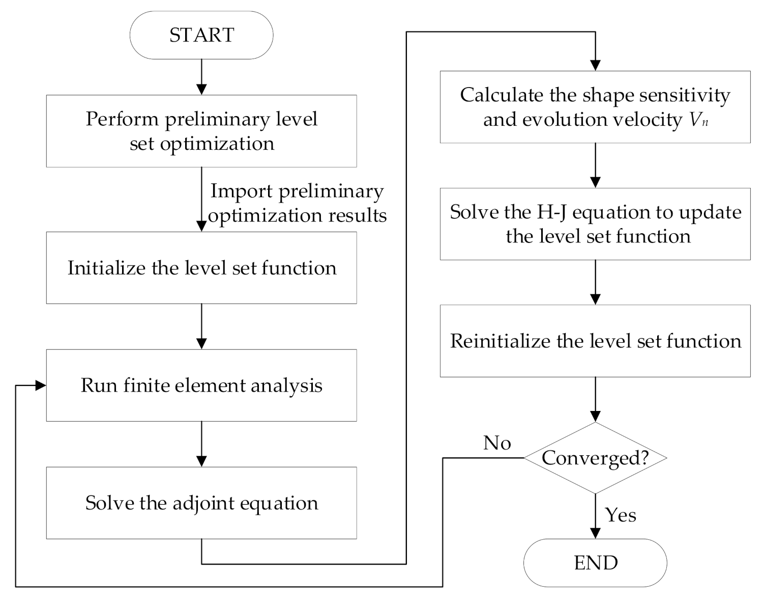
5. Optimization Procedure

In this paper, the Lagrangian method is used to solve the level set topology optimization problem (40), which transforms the optimization problem into the Lagrangian unconstrained minimization problem. The topology optimization problem is transformed into:

$$\begin{array}{c}L\left(\mathsf{\Omega },\ell ,\gamma \right)=J\left(\mathsf{\Omega }\right)-{\ell }_1{C}_p\left(\mathsf{\Omega }\right)-{\ell }_2\left(Vol\left(\mathsf{\Omega }\right)-V_{max}\right)\\ +\frac{{\gamma }_1}{2}{\left(C_p\left(\mathsf{\Omega }\right)\right)}^2+\frac{{\gamma }_2}{2}{\left(Vol\left(\mathsf{\Omega }\right)-V_{max}\right)}^2\end{array}$$

(52)

where $\ell =\left({\ell }_1,{\ell }_2\right)$ and γ = (γ₁, γ₂) are the Lagrangian multipliers and the penalty factors of the constraint function, respectively.

The shape sensitivity of the augmented Lagrangian function can be derived as:

$$\begin{array}{c}{L}^{\prime }\left(\mathsf{\Omega },\ell ,\gamma \right)\left(\theta \right)=J^{\prime }\left(\mathsf{\Omega }\right)\left(\theta \right)-{\ell }_1{C}_p^{\prime }\left(\mathsf{\Omega }\right)\left(\theta \right)-{\ell }_2{{\displaystyle \int }}_{\mathsf{\Omega }}^{}\theta ·nds+{\gamma }_1{C}_p\left(\mathsf{\Omega }\right)C_p^{\prime }\left(\mathsf{\Omega }\right)\left(\theta \right)\\ +{\gamma }_2\left(Vol\left(\mathsf{\Omega }\right)-V_{max}\right){{\displaystyle \int }}_{\mathsf{\Omega }}^{}\theta ·nds \end{array}$$

(53)

Substituting J’(Ω)(θ) and C’_p(Ω)(θ), the normal evolution velocity V_n of the Hamilton–Jacobi equation can be obtained.

When performing a one-step solution, it is easy to make the optimization considering the effects of porosity converge to the local optimal solution. Addressing the issue, the topology optimization is solved in two steps in this paper. For one thing, the hole nucleation method combining BESO and topological sensitivity can be used to reduce the influence of initial hole distribution on the optimization results. For another, the optimization results obtained in the previous step can be directly used in the second step, which improves the convergence efficiency of the optimization. Therefore, the level set topology optimization algorithm considering porosity constraints is summarized as follows:

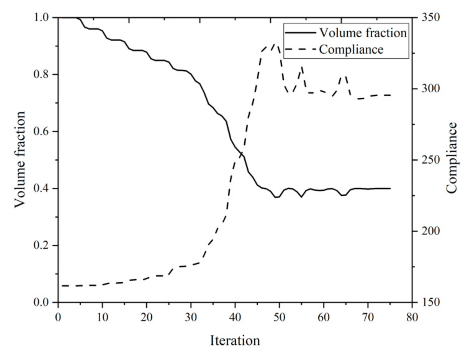
• Perform preliminary structural optimization according to the level set topology optimization combining BESO and topological sensitivity and obtain optimal results without considering porosity constraints;
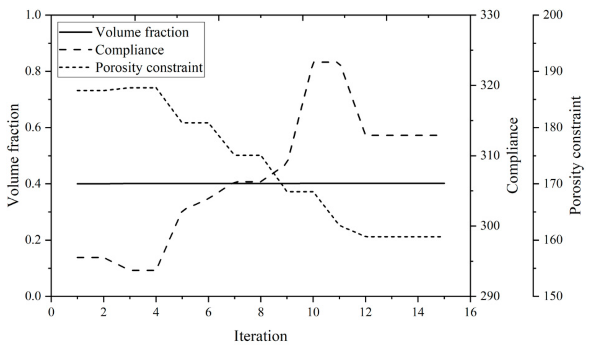
• Import optimization results without considering porosity constraints for subsequent optimization;
• Initialize the level set function Φ₂ according to the preliminary optimization results;
• According to the given load conditions, solving the elastic balance equation a(u, v, Φ) = L(v, Φ), the displacement field vector u_Ω and the topological sensitivity D_T J(Ω) are obtained;
• Solve the adjoint vector p_Ω using (49);
• Calculate the shape sensitivity using (48);
• Solve the level set velocity field vector Vn, and extend the velocity to the entire design domain Ω;
• Using the existing level set function and the obtained velocity Vn, solve the Hamilton–Jacobi equation $\frac{\partial \Phi }{\partial t}-V_n\Vert \nabla \Phi \Vert =0$ by finite difference to obtain a new level set function;
• Reinitialize the signed distance function for the new level set function;
• Check whether the level set function satisfies the convergence criterion. If not, repeat steps 4 to 10 until convergence. The convergence criterion is:

  $$\left|J^n-J^{n-k}\right|\le 0.01J^n \&\& \left|C_p^n-C_p^{n-k}\right|\le 0.01C^n \&\& \left|V^n-V_{max}\right|\le 0.01$$

  (54)

  where 1 ≤ k ≤ 5.

The optimization process of level set topology optimization considering porosity constraints is shown in Figure 2.

6. Numerical Examples

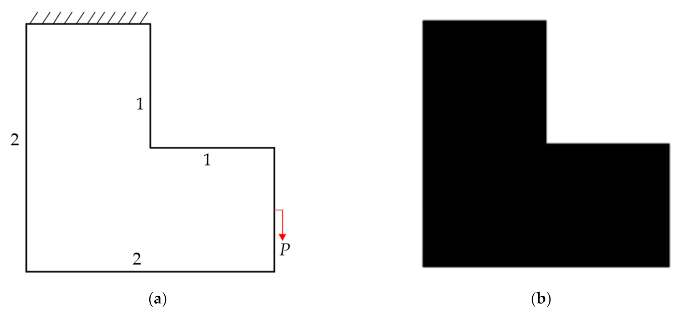
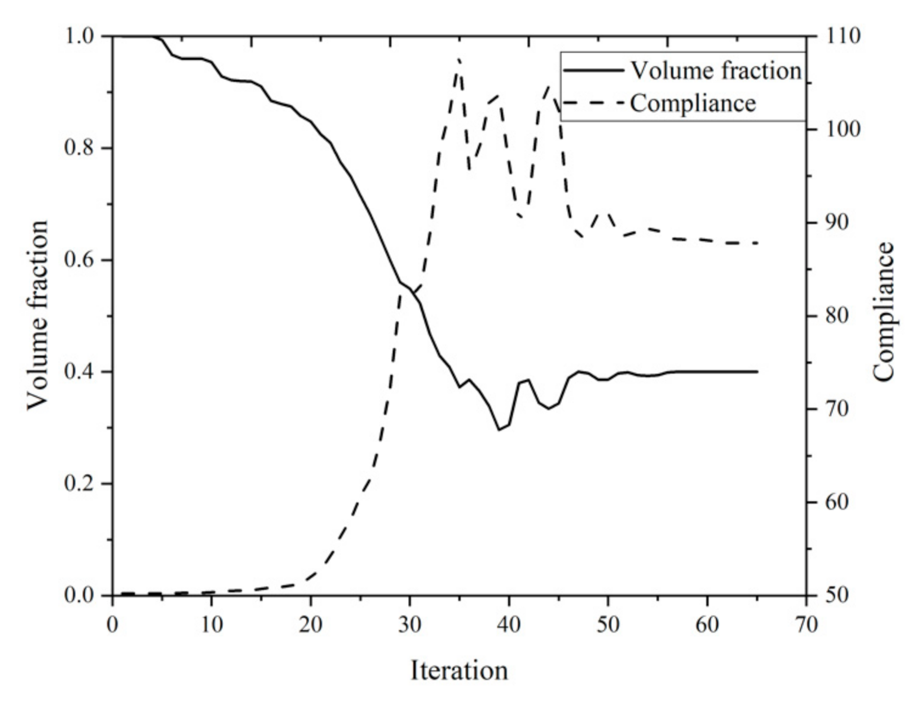
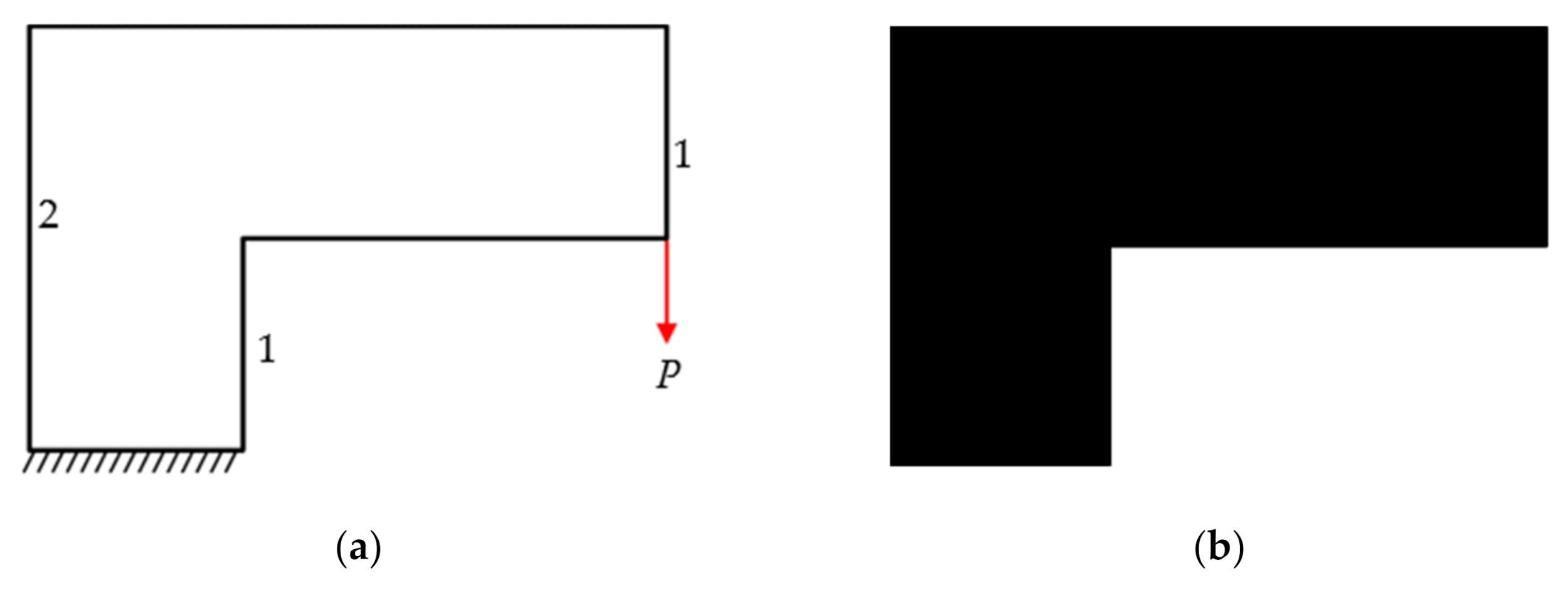
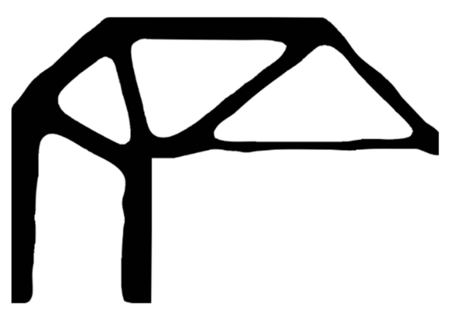
In this Section, two examples are given to verify the effectiveness of the proposed porosity constraints. For the convenience of calculation, the measure M(B_x,r) of the small pores is expressed as:

$$M\left(B_{x,r}\right)=\pi r^d$$

(55)

where d represents the structural dimension.

The Lagrangian multipliers and the penalty factors of (53) will be updated continuously with the rule:

$$\begin{array}{c}{\ell }_1^{n+1}={\ell }_1^n-{\gamma }_1^n{C}_p^n\left(\mathsf{\Omega }\right) \\ {\ell }_2^{n+1}={\ell }_2^n-{\gamma }_2^n\left(Vo{l}^n\left(\mathsf{\Omega }\right)-V_{max}\right)\\ {\gamma }_1^{n+1}={\beta }_1{\gamma }_1^n \\ {\gamma }_2^{n+1}={\beta }_2{\gamma }_2^n \end{array}$$

(56)

where $\ell =\left({\ell }_1,{\ell }_2\right)$ is updated every iteration and γ = (γ₁, γ₂) is updated every five iterations. In the level set topology optimization, it is difficult to select the initial values of Lagrangian multipliers and the penalty factors. The initial values of the following numerical examples follow the empirical formula:

$$\begin{array}{c}{\ell }_1^0=0.05\left(J\left(\mathsf{\Omega }\right)/V_{max}\right) \\ {\ell }_2^0=0.05\left(C_p\left(\mathsf{\Omega }\right)/V_{max}\right)\\ {\gamma }_1^0=0.05\left|{\ell }_1^0\right| \\ {\gamma }_2^0=0.05\left|{\ell }_2^0\right| \end{array}$$

(57)

Since the main purpose of this Section is to verify the effectiveness of the method, all material properties and loads are dimensionless. The materials for all numerical examples are isotropic. Assume that the Young’s modulus of the solid material is E₁ = 1, the Young’s modulus of the void material is E₀ = 10⁻³, and the Poisson’s ratio is ϑ = 0.3. All examples adopt four-node rectangular elements to mesh the design domain.

6.1. L-Shaped Beam

The design domain of this optimization problem is an L-shaped area with a ratio 1:1 of length L to height H, meshed with 4800 elements, as shown in Figure 3a. Its upper side is fixed, and a vertical load P = 1 is applied at the middle of its right-hand side. The upper bound of volume ratio is 0.4. The evolutionary volume ratio c_er is set to 0.04, the filter radius R_min is taken as 3, and the interval j of hole nucleation is 5. The initial shape is displayed in Figure 3b. At first, the level set topology optimization of hole nucleation combining BESO and topological sensitivity is employed. The optimized shape is shown in Figure 4. The optimization converges after 65 iterations, and the evolution of the volume fraction and the compliance are shown in Figure 5.

Secondly, the level set topology optimization considering porosity constraint is employed. The preliminary optimization results of the previous step are imported to perform topology optimization considering porosity constraint. The pores radius r is set to 0.625, and the tolerance η is taken as 0.3. The optimization converges after 14 iterations, and the evolution of the volume fraction, the compliance and porosity constraint are shown in Figure 6. The preliminary optimization results and the optimization results considering porosity constraint are shown in Figure 7a,b, respectively, and the corresponding porosity constraint distribution clouds are shown in Figure 7c,d.

As shown in Figure 6, the optimization problem with porosity constraints converges after 14 iterations, the porosity constraint value decreases 30% from 14.6, but the objective compliance increases from 87.8 to 93.5. Without considering the porosity constraint, the maximum porosity constraint value appears near the reentrant corner of the optimization result shown in Figure 7c, while the porosity constraint value in other areas is almost zero. According to practical experience, the reentrant corner is easy to produce stress concentration under the loads. If there are pores in this area during manufacturing, cracks will be generated under the action of concentrated force, which will reduce the fatigue performance of parts. Therefore, the reentrant corner is more sensitive to porosity. If the reentrant corner is smoothed into a rounded area, the stress concentration can be effectively reduced, and the sensitivity to the porosity is also reduced. Therefore, under the effect of porosity constraints, the reentrant corner will be key optimization region of the structure. According to the optimization result in Figure 7d, under the effect of porosity constraints, the reentrant corner becomes smooth and presents a characteristic of fillet, while the other regions almost have no change. By observing the corresponding porosity constraint value in this area, it can be found that the porosity constraint value has decreased significantly, and the maximum porosity constraint value in this area has decreased from 1.92 to 1.14. According to the numerical analysis, the topology optimization method considering porosity constraints is effective and conforms to the actual situation. Comparing the changes in compliance with or without considering porosity constraint, there is a deviation that is within the admissible range.

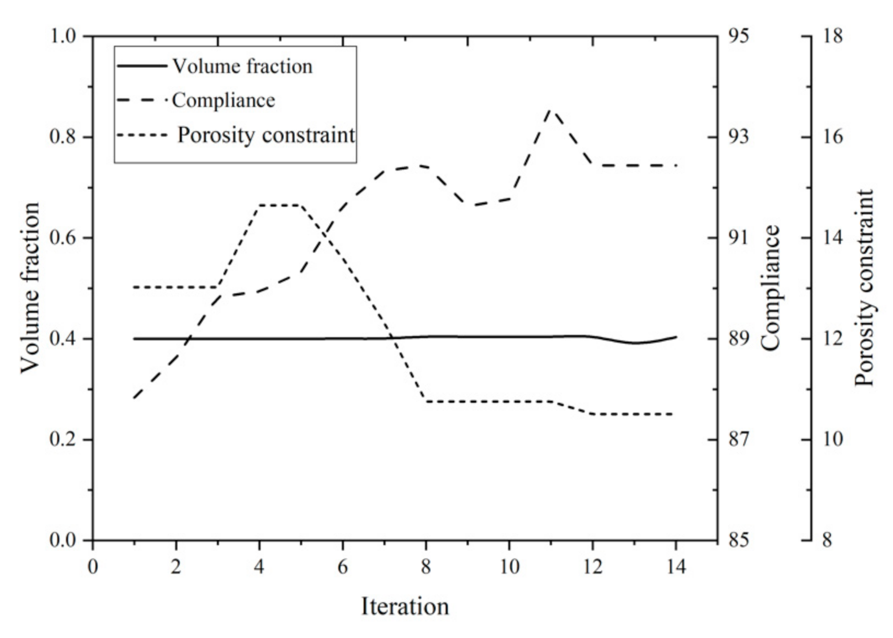
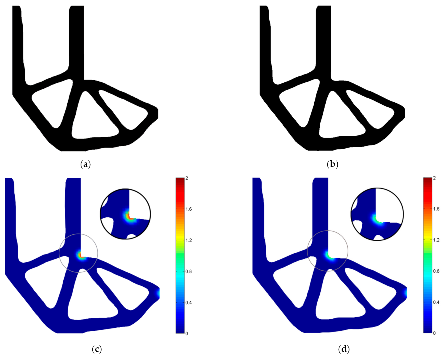
6.2. C-Shaped Bracket

The design domain of the second example is a C-shaped area with a ratio 3:2 of length L to height H, meshed with 3600 elements, as shown in Figure 8a. Its lower side is fixed, and a vertical load P = 1 is applied at the bottom of its right-hand side. The upper bound of volume ratio is 0.4. The evolutionary volume ratio c_er is set to 0.04, the filter radius R_min is taken as 3, and the interval j of hole nucleation is 5. The initial shape is displayed in Figure 8b. At first, the level set topology optimization of hole nucleation combining BESO and topological sensitivity is employed. The optimized shape is shown in Figure 9. The optimization converges after 75 iterations, and the evolution of the volume fraction and the compliance are shown in Figure 10.

Secondly, the preliminary optimization results of C-shaped bracket are imported to perform topology optimization considering the porosity constraint. The pores radius r is set to 0.5, and the tolerance η is taken as 0.15. The optimization converges after 15 iterations, and the evolution of the volume fraction, the compliance, and porosity constraint are shown in Figure 11. The preliminary optimization results and the optimization results considering porosity constraint are shown in Figure 12a,b, respectively, and the corresponding porosity constraint distribution clouds are shown in Figure 12c,d.

As shown in Figure 11, the optimization problem with porosity constraints converges after 15 iterations, the porosity constraint value decreases 15% from 187.1, but the objective compliance increases from 293.7 to 323.3. Without considering the porosity constraint, the maximum porosity constraint value appears near the reentrant corner of the optimization result shown in Figure 12c, while the porosity constraint value in other areas is almost zero. Therefore, under the effect of porosity constraints, the reentrant corner will be key optimization region of the structure. According to the optimization results of Figure 12d, under the effect of porosity constraint, the reentrant corner becomes smooth and presents a characteristic of fillet. The results show that the porosity constraint value decreases obviously, and the maximum value decreases from 18.9 to 10.4. Comparing the changes in compliance with or without considering porosity constraint, there is a deviation that is within the admissible range. The optimization results of the C-shaped bracket are similar to the L-shaped beam, which further proves the effectiveness of the proposed method.

7. Conclusions

Porosity is one of the main defects of the manufactured parts by AM. The appearance of porosity will significantly reduce the mechanical and fatigue properties of fabricated parts and accelerate the failure of parts. To reduce the influence of porosity, the pores are considered in topology optimization for AM so as to obtain a robust optimization result. In this paper, the concept of topological sensitivity is used to establish the global porosity constraint function, and the shape sensitivity of the porosity constraint is analyzed. Considering the robustness of the algorithm, the topology optimization considering the porosity constraint is performed by two steps. In the preliminary optimization of the structure, a hole nucleation method combining BESO and topological sensitivity is proposed to solve the problem that the level set topology optimization method cannot automatically nucleate holes. Next, the preliminary optimization results are subjected to topology optimization considering porosity constraint, obtaining the results that can reduce the effects of porosity on structural performance. In the L-shaped beam, the porosity constraint value of the optimization results is reduced by 30%. In the C-shaped bracket, the value is reduced by 15%, but the compliance of the structural performance is only slightly increased. Compared with the decrease of porosity constraint value, the change of compliance is very small and within the admissible range. The step-by-step optimization method proposed in this paper will not increase the extra workload for engineers to guess the initial structure and improve the convergence efficiency of the optimization algorithm. This method provides a potential solution for multi-constraint topology optimization problems. In future work, the idea of using topological sensitivity to construct porosity constraints can also be used to consider additive manufacturing defects such as cracks and spheroidization in topology optimization, which further broadens the research field of topology optimization for additive manufacturing defects.

References

1. Allaire, G.; Jouve, F. Structural Optimization by the Homogenization Method; Springer: Dordrecht, The Netherlands, 1999; pp. 293–300. [Google Scholar]
2. Bendsøe, M.P.; Kikuchi, N. Generating optimal topologies in structural design using a homogenization method. Comput. Methods Appl. Mech. Eng. 1988, 71, 197–224. [Google Scholar] [CrossRef]
3. Díaz, A.R.; Bendsøe, M.P. Shape optimization of structures for multiple loading conditions using a homogenization method. Struct. Optim. 1992, 4, 17–22. [Google Scholar] [CrossRef]
4. Suzuki, K.; Kikuchi, N. A homogenization method for shape and topology optimization. Comput. Methods Appl. Mech. Eng. 1991, 93, 291–318. [Google Scholar] [CrossRef] [Green Version]
5. Yoo, J.; Kikuchi, N.; Volakis, J.L. Structural optimization in magnetic fields using the homogenization design method—Part I. Arch. Comput. Methods Eng. 2001, 8, 387–406. [Google Scholar] [CrossRef]
6. Bendsøe, M.P.; Sigmund, O. Material interpolation schemes in topology optimization. Arch. Appl. Mech. 1999, 69, 635–654. [Google Scholar] [CrossRef]
7. Rietz, A. Sufficiency of a finite exponent in SIMP (power law) methods. Struct. Multidiscip. Optim. 2001, 21, 159–163. [Google Scholar] [CrossRef]
8. Sigmund, O. A 99 line topology optimization code written in Matlab. Struct. Multidiscip. Optim. 2001, 21, 120–127. [Google Scholar] [CrossRef]
9. Stolpe, M.; Svanberg, K. An alternative interpolation scheme for minimum compliance topology optimization. Struct. Multidiscip. Optim. 2001, 22, 116–124. [Google Scholar] [CrossRef]
10. Huang, X.; Xie, Y.M. Convergent and mesh-independent solutions for the bi-directional evolutionary structural optimization method. Finite Elem. Anal. Des. 2007, 43, 1039–1049. [Google Scholar] [CrossRef]
11. Huang, X.; Xie, Y.M. A new look at ESO and BESO optimization methods. Struct. Multidiscip. Optim. 2008, 35, 89–92. [Google Scholar] [CrossRef]
12. Xia, L.; Xia, Q.; Huang, X.; Xie, Y.M. Bi-directional Evolutionary Structural Optimization on Advanced Structures and Materials: A Comprehensive Review. Arch. Comput. Methods Eng. 2018, 25, 437–478. [Google Scholar] [CrossRef]
13. Xie, Y.M.; Steven, G.P. A simple evolutionary procedure for structural optimization. Comput. Struct. 1993, 49, 885–896. [Google Scholar] [CrossRef]
14. Yang, X.Y.; Xie, Y.M.; Steven, G.P.; Querin, O.M. Bidirectional Evolutionary Method for Stiffness Optimization. AIAA J. 1999, 37, 1483–1488. [Google Scholar] [CrossRef]
15. Guo, X.; Zhang, W.; Zhang, J.; Yuan, J. Explicit structural topology optimization based on moving morphable components (MMC) with curved skeletons. Comput. Methods Appl. Mech. Eng. 2016, 310, 711–748. [Google Scholar] [CrossRef]
16. Guo, X.; Zhang, W.; Zhong, W. Doing Topology Optimization Explicitly and Geometrically—A New Moving Morphable Components Based Framework. J. Appl. Mech. 2014, 81, 081009. [Google Scholar] [CrossRef]
17. Zhang, W.; Li, D.; Zhang, J.; Guo, X. Minimum length scale control in structural topology optimization based on the Moving Morphable Components (MMC) approach. Comput. Methods Appl. Mech. Eng. 2016, 311, 327–355. [Google Scholar] [CrossRef]
18. Zhang, W.; Yuan, J.; Zhang, J.; Guo, X. A new topology optimization approach based on Moving Morphable Components (MMC) and the ersatz material model. Struct. Multidiscip. Optim. 2016, 53, 1243–1260. [Google Scholar] [CrossRef]
19. Allaire, G.; Jouve, F.; Toader, A.-M. A level-set method for shape optimization. Comptes Rendus Math. 2002, 334, 1125–1130. [Google Scholar] [CrossRef]
20. Allaire, G.; Jouve, F.; Toader, A.-M. Structural optimization using sensitivity analysis and a level-set method. J. Comput. Phys. 2004, 194, 363–393. [Google Scholar] [CrossRef] [Green Version]
21. Challis, V. A discrete level-set topology optimization code written in matlab. Struct. Multidiscip. Optim. 2010, 41, 453–464. [Google Scholar] [CrossRef]
22. Otomori, M.; Yamada, T.; Izui, K.; Nishiwaki, S. Matlab code for a level set-based topology optimization method using a reaction diffusion equation. Struct. Multidiscip. Optim. 2015, 51, 1159–1172. [Google Scholar] [CrossRef] [Green Version]
23. Sethian, J.A.; Wiegmann, A. Structural Boundary Design via Level Set and Immersed Interface Methods. J. Comput. Phys. 2000, 163, 489–528. [Google Scholar] [CrossRef]
24. Van Dijk, N.P.; Maute, K.; Langelaar, M.; van Keulen, F. Level-set methods for structural topology optimization: A review. Struct. Multidiscip. Optim. 2013, 48, 437–472. [Google Scholar] [CrossRef]
25. Wang, M.Y.; Wang, X.; Guo, D. A level set method for structural topology optimization. Comput. Methods Appl. Mech. Eng. 2003, 192, 227–246. [Google Scholar] [CrossRef]
26. Calleja-Ochoa, A.; Gonzalez-Barrio, H.; Lopez de Lacalle, N.; Martinez, S.; Albizuri, J.; Lamikiz, A. A New Approach in the Design of Microstructured Ultralight Components to Achieve Maximum Functional Performance. Materials 2021, 14, 1588. [Google Scholar] [CrossRef]
27. Aboulkhair, N.T.; Everitt, N.M.; Ashcroft, I.; Tuck, C. Reducing porosity in AlSi10Mg parts processed by selective laser melting. Additive Manuf. 2014, 1–4, 77–86. [Google Scholar] [CrossRef]
28. Bartlett, J.L.; Heim, F.M.; Murty, Y.V.; Li, X. In situ defect detection in selective laser melting via full-field infrared thermography. Addit. Manuf. 2018, 24, 595–605. [Google Scholar] [CrossRef]
29. Gong, H.; Rafi, H.; Nadimpalli, K.; Starr, T.; Stucker, B. Defect Morphology in Ti-6Al-4V Parts Fabricated by Selective Laser Melting and Electron Beam Melting. In Proceedings of the 24th Annual International Solid Freeform Fabrication Symposium, Austin, TX, USA, 12–14 August 2013. [Google Scholar]
30. Gong, H.; Rafi, K.; Gu, H.; Janaki Ram, G.D.; Starr, T.; Stucker, B. Influence of defects on mechanical properties of Ti–6Al–4V components produced by selective laser melting and electron beam melting. Mater. Design 2015, 86, 545–554. [Google Scholar] [CrossRef]
31. Gu, D.; Hagedorn, Y.-C.; Meiners, W.; Meng, G.; Batista, R.J.S.; Wissenbach, K.; Poprawe, R. Densification behavior, microstructure evolution, and wear performance of selective laser melting processed commercially pure titanium. Acta Mater. 2012, 60, 3849–3860. [Google Scholar] [CrossRef]
32. Li, R.; Liu, J.; Shi, Y.; Du, M.; Xie, Z. 316L Stainless Steel with Gradient Porosity Fabricated by Selective Laser Melting. J. Mater. Eng. Perform. 2010, 19, 666–671. [Google Scholar] [CrossRef]
33. Liu, Q.C.; Elambasseril, J.; Sun, S.J.; Leary, M.; Brandt, M.; Sharp, P.K. The Effect of Manufacturing Defects on the Fatigue Behaviour of Ti-6Al-4V Specimens Fabricated Using Selective Laser Melting. Adv. Mater. Res. 2014, 891–892, 1519–1524. [Google Scholar] [CrossRef]
34. Zhu, L.; Xue, P.; Lan, Q.; Meng, G.; Ren, Y.; Yang, Z.; Xu, P.; Liu, Z. Recent research and development status of laser cladding: A review. Opt. Laser Technol. 2021, 138, 106915. [Google Scholar] [CrossRef]
35. Calleja, A.; Tabernero, I.; Ealo, J.A.; Campa, F.J.; Lamikiz, A.; de Lacalle, L.N.L. Feed rate calculation algorithm for the homogeneous material deposition of blisk blades by 5-axis laser cladding. Int. J. Adv. Manuf. Technol. 2014, 74, 1219–1228. [Google Scholar] [CrossRef]
36. Gong, H.; Rafi, K.; Gu, H.; Starr, T.; Stucker, B. Analysis of defect generation in Ti–6Al–4V parts made using powder bed fusion additive manufacturing processes. Addit. Manuf. 2014, 1–4, 87–98. [Google Scholar]
37. Qiu, C.; Adkins, N.J.E.; Attallah, M.M. Microstructure and tensile properties of selectively laser-melted and of HIPed laser-melted Ti–6Al–4V. Mater. Sci. Eng. A 2013, 578, 230–239. [Google Scholar] [CrossRef]
38. Thijs, L.; Verhaeghe, F.; Craeghs, T.; Humbeeck, J.V.; Kruth, J.-P. A study of the microstructural evolution during selective laser melting of Ti–6Al–4V. Acta Mater. 2010, 58, 3303–3312. [Google Scholar] [CrossRef]
39. Vilaro, T.; Colin, C.; Bartout, J.D. As-Fabricated and Heat-Treated Microstructures of the Ti-6Al-4V Alloy Processed by Selective Laser Melting. Metall. Mater. Trans. A 2011, 42, 3190–3199. [Google Scholar] [CrossRef]
40. Gäumann, M.; Henry, S.; Cléton, F.; Wagnière, J.D.; Kurz, W. Epitaxial laser metal forming: Analysis of microstructure formation. Mater. Sci. Eng. A 1999, 271, 232–241. [Google Scholar] [CrossRef]
41. Clijsters, S.; Craeghs, T.; Buls, S.; Kempen, K.; Kruth, J.P. In situ quality control of the selective laser melting process using a high-speed, real-time melt pool monitoring system. Int. J. Adv. Manuf. Technol. 2014, 75, 1089–1101. [Google Scholar] [CrossRef]
42. Allaire, G.; de Gournay, F.; Jouve, F.; Toader, A.-M. Structural optimization using topological and shape sensitivity via a level set method. Control Cybern. 2005, 34, 59. [Google Scholar]
43. He, L.; Kao, C.-Y.; Osher, S. Incorporating topological derivatives into shape derivatives based level set methods. J. Comput. Phys. 2007, 225, 891–909. [Google Scholar] [CrossRef]
44. Xia, Q.; Shi, T.; Xia, L. Stable hole nucleation in level set based topology optimization by using the material removal scheme of BESO. Comput. Methods Appl. Mech. Eng. 2019, 343, 438–452. [Google Scholar] [CrossRef]
45. Yaghmaei, M.; Ghoddosian, A.; Khatibi, M.M. A filter-based level set topology optimization method using a 62-line MATLAB code. Struct. Multidiscip. Optim. 2020, 62, 1001–1018. [Google Scholar] [CrossRef]
46. Simon, J. Differentiation with Respect to the Domain in Boundary Value Problems. Numer. Funct. Anal. Optim. 1980, 2, 649–687. [Google Scholar] [CrossRef]
47. Giusti, S.M.; Novotny, A.A.; Padra, C. Topological sensitivity analysis of inclusion in two-dimensional linear elasticity. Eng. Anal. Bound. Elem. 2008, 32, 926–935. [Google Scholar] [CrossRef]
48. Novotny, A.A.; Feijóo, R.A.; Taroco, E.; Padra, C. Topological sensitivity analysis. Comput. Methods Appl. Mech. Eng. 2003, 192, 803–829. [Google Scholar] [CrossRef]
49. Martínez-Frutos, J.; Allaire, G.; Dapogny, C.; Periago, F. Structural optimization under internal porosity constraints using topological derivatives. Comput. Methods Appl. Mech. Eng. 2019, 345, 1–25. [Google Scholar] [CrossRef] [Green Version]
50. Allaire, G.; Jouve, F.; Michailidis, G. Thickness control in structural optimization via a level set method. Struct. Multidiscip. Optim. 2016, 53, 1349–1382. [Google Scholar] [CrossRef] [Green Version]
Figure 1. Flowchart of the level set topology optimization combining BESO and topological sensitivity.
Applsci 11 05578 g001
Figure 2. Flowchart of the level set topology optimization considering porosity constraints.
Applsci 11 05578 g002
Figure 3. Optimum design problem of L-shaped beam, (a) design domain and boundary conditions; (b) initial shape.
Applsci 11 05578 g003
Figure 4. Preliminary optimized shape of L-shaped beam.
Applsci 11 05578 g004
Figure 5. Convergence history of L-shaped beam by hole nucleation method.
Applsci 11 05578 g005
Figure 6. Convergence history of L-shaped beam considering porosity constraint.
Applsci 11 05578 g006
Figure 7. Optimization results and porosity constraint distribution clouds of L-shaped beam, (a) optimized shape without considering porosity constraint; (b) optimized shape considering porosity constraint; (c) porosity constraint distribution clouds without considering porosity constraint; (d) porosity constraint distribution clouds considering porosity constraint.
Applsci 11 05578 g007
Figure 8. Optimum design problem of C-shaped bracket, (a) design domain and boundary conditions; (b) initial shape.
Applsci 11 05578 g008
Figure 9. Preliminary optimized shape of C-shaped bracket.
Applsci 11 05578 g009
Figure 10. Convergence history of C-shaped bracket by hole nucleation method.
Applsci 11 05578 g010
Figure 11. Convergence history of C-shaped bracket considering porosity constraint.
Applsci 11 05578 g011
Figure 12. Optimization results and porosity constraint distribution clouds of C-shaped bracket, (a) optimized shape without considering porosity constraint; (b) optimized shape considering porosity constraint; (c) porosity constraint distribution clouds without considering porosity constraint; (d) porosity constraint distribution clouds considering porosity constraint.
Applsci 11 05578 g012
Publisher’s Note: MDPI stays neutral with regard to jurisdictional claims in published maps and institutional affiliations.