Article

Effect of Blade Leading and Trailing Edge Configurations on the Performance of a Micro Tubular Propeller Turbine Using Response Surface Methodology

1
Graduate School of Mechanical Engineering, Sungkyunkwan University, Suwon 16419, Korea
2
School of Mechanical Engineering, Sungkyunkwan University, Suwon 16419, Korea
*
Author to whom correspondence should be addressed.
Appl. Sci. 2021, 11(12), 5596; https://doi.org/10.3390/app11125596
Submission received: 22 April 2021 / Revised: 14 June 2021 / Accepted: 15 June 2021 / Published: 17 June 2021

Abstract

:
With the recent rise in importance of environmental issues, research on micro hydropower, a kind of renewable energy source, is being actively conducted. In this study, a micro tubular propeller turbine was selected for study of micro hydropower in pipes. Numerical analysis was conducted to evaluate the performance. Response surface methodology using design of experiments was performed to efficiently investigate the effect of the blade leading and trailing edge elliptic aspect ratios on the performance. The trailing edge configuration was found to be more related to the performance, because of the drastic pressure variation due to the stagnation point formed, regardless of the leading edge configuration. To improve the performance, a NACA airfoil was introduced. The results show that the flow became more stable than the reference model, and the efficiency was increased by 2.44%.

1. Introduction

In 2015, the Paris Agreement was adopted to reduce greenhouse gas emissions as climate change was becoming a more serious problem worldwide [1]. However, even after the adoption of the treaty, global greenhouse gas emissions have been increasing year by year, and are projected to increase in the future [2]. Greenhouse gases emitted worldwide mostly come from the energy sector (73%), and in particular, the energy use in industry accounts for 24%, which is the largest part [3,4]. Therefore, it is urgent to replace fossil fuel energy with clean energy that does not produce carbon dioxide; but in 2019, renewable energy accounted for only 27.3% of the global energy production [5]. Hence, the importance of renewable energy is expected to increase further.
Renewable energy, which is often referred to as clean energy, is defined to be energy collected from renewable sources. It includes hydropower, solar energy, wind energy, biomass energy and geothermal energy [6,7]. In 2019, hydropower accounted for 50% of the total renewable energy capacity across the globe [8]. This indicates that hydropower has steadily gained ground in the renewable energy market. However, only a fraction of the hydropower energy potential is currently being developed and used [9]. Accordingly, it is necessary to further research hydropower.
Hydropower generates electricity by rotating a hydro turbine using a head of the water, and it has the advantage that it does not produce carbon dioxide at all, while offering high energy density [10]. Micro hydropower, which is typically classified as hydropower with less than 100 kW of installed capacity [11,12], has the advantage of longer life, lower operation costs, and fewer restrictions on space, relative to macro hydropower [13]. In particular, the in-line type hydro turbine for micro hydropower is highly safe and sustainable, because regardless of the external environment, it can supply water at a constant flow rate [13,14]. In addition, it can be applied to wherever there is a pipeline, such as water and sewage, agricultural water, plant cooling water, and high-rise building drainage.
Research on the in-line type hydro turbine for micro hydropower has been conducted for many years, and various types of hydro turbine have been proposed. Since the in-line type turbine is a reaction turbine that utilizes pressure energy remaining in the pipe, classical turbines such as Francis and Kaplan turbines for small hydropower have been researched [15,16,17,18]. A pump as turbine (PAT) is also known to be suitable for small hydropower applications [19] and has been investigated in a variety of forms such as mixed flow or centrifugal types [20,21]. Furthermore, in addition to classic turbines, many new types of turbines have been developed. Chen et al. [22] developed a vertical axis turbine to generate power from water pipelines, and conducted numerical analysis and experimental tests for over 20 models through design variables, such as drag-type or lift-type turbine, and deflector configurations. Payambarpour et al. [23] used a Savonius turbine as an in-line type hydro turbine, and improved the performance by adjusting design variables, such as deflector configurations and aspect ratio, through numerical analysis and experiments. A helical turbine, known as the Gorlov vertical axis turbine, was introduced into the LucidPipeTM system to generate energy [24]. Yeo et al. [25] studied a vertical axis turbine based on a helical turbine numerically, and investigated the effect of tip-speed ratios on the performance. A hydrocoil turbine, which is an in-line type turbine version of the Archimedes screw turbine, was developed by HydroCoil Power, Inc. [26]. Sinagra et al. [27] adopted an in-line type crossflow turbine for pressure regulation and energy production, and verified the performance through numerical and experimental analysis. Research on contra-rotating turbines for micro hydropower was conducted, and the performance was evaluated through numerical analysis and experiments [28,29].
Among the various types of in-line type turbines, a micro tubular propeller turbine was selected for this study. A tubular turbine, often referred to as a bulb turbine, is a kind of axial turbine that is usually used in low head conditions. Unlike a propeller or Kaplan turbine, the tubular turbine does not have a spiral casing, and so it is easy to design an in-line hydro turbine [30]. Studies on hydropower using the tubular turbine have been actively conducted before [31,32,33]. However, typical tubular turbines have the disadvantage of complicated structures with generators installed inside the pipes and maintenance problems due to clogging [34]. Samora et al. [35] designed a micro tubular propeller turbine that can be installed in pipes with a diameter of less than 200 mm. It is a miniaturized tubular turbine whose generator is located outside the pipe like an S-turbine. In addition, it does not include a guide vane, so it has the advantage of a simpler configuration and reduction of clogging issues, enabling easier maintenance. In this study, the effect of blade configuration variation on performance was investigated through numerical analysis, and it was expected that modifying the blade configuration would improve the performance.

2. Numerical Analysis

2.1. Model Description

A reference model of the micro tubular propeller turbine was designed referring to the precedent study [35]. Figure 1 and Figure 2 show a system schematic and a runner model, respectively, and Table 1 describes the specification. The design of an in-line type hydro turbine while locating the generator outside of the flow path necessitates the use of bent pipes. The bend angle of the pipe is set to 45° to minimize the head loss inevitably generated.

2.2. Evaluation Indicator

Among the output values obtained from numerical analysis, the value adopted as an indicator to evaluate the performance is efficiency. The hydraulic efficiency of the hydro turbine can be calculated as the ratio of the mechanical power generated by the turbine shaft to the maximum power that can be available at the inlet of the runner, as indicated in Equation (3) [36]. Here, the mechanical power can be obtained by multiplying the axial torque and rotational speed, as expressed in Equation (1). In addition, the maximum power available at the runner inlet can be acquired by the product of the density of the working fluid, the gravitational acceleration, the flow rate, and the head. In this case, the head can be obtained using the difference of static pressure, Δ p at the inlet and outlet of the runner, as described in Equation (2).
P = T N
H = Δ p ρ g
η = P ρ g Q H
where the terms are as defined in the nomenclature below.

2.3. Grid Generation

For numerical analysis, the model representing the fluid zone of the micro tubular propeller turbine system was constructed with a grid system. The pipe part was composed of a mixture of structured and unstructured mesh using ANSYS Mesh, and the runner part was composed of structured mesh using ANSYS TurboGrid. To resolve the problem of node mismatch at the interface between pipe and runner, the grid at the interface was densely generated. Y-plus is the dimensionless wall distance, which can be calculated as y + = ρ y u τ μ where ρ is the working fluid density, μ is the working fluid dynamic viscosity, y is the wall distance, u τ = τ w ρ is the wall shear velocity, and τ w is the wall shear stress. In this study, y-plus was limited below 2 to consider the shear stress on the wall, such as blades.
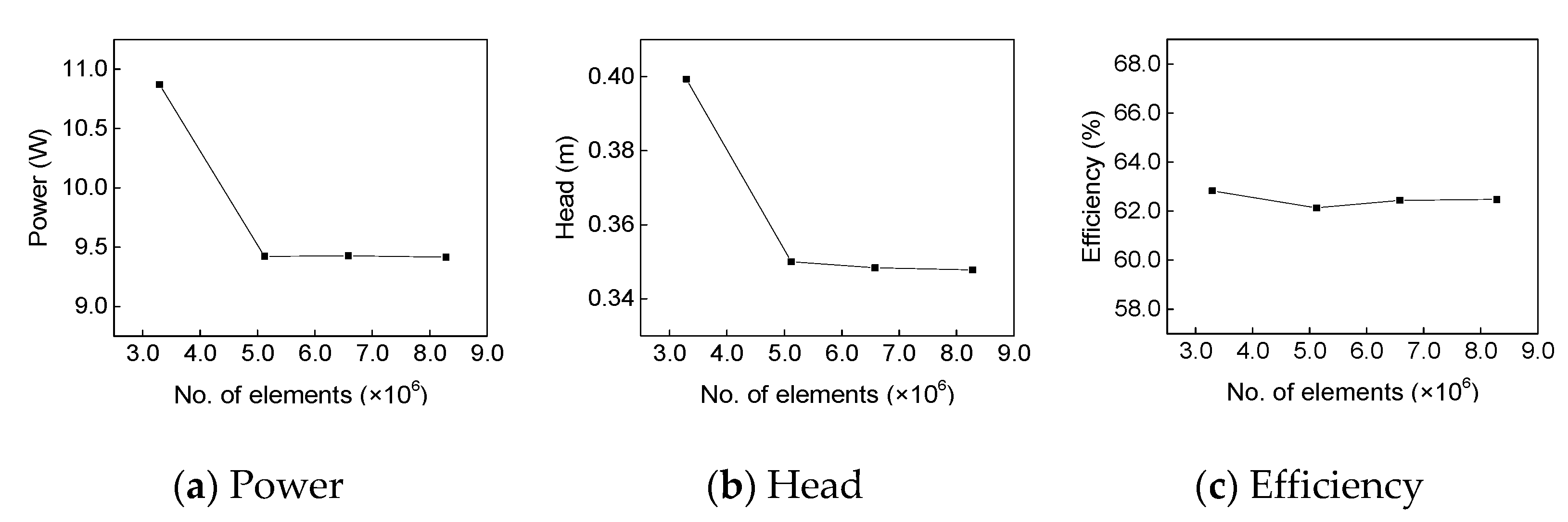
A grid dependency test was performed to minimize the effect of the grid size on the results, and consider the economics of the numerical analysis time. Figure 3 shows the results of the variation in the power, head, and efficiency represented in Equations (1)–(3) by the number of elements. The results show that those values do not change greatly from more than about 5 million grid elements. Therefore, the number of grid elements used in this study was set to approximately 5 million.

2.4. Boundary Conditions

A numerical analysis was conducted using ANSYS CFX ver. 2020 R2, and Table 2 describes the boundary conditions applied in this study. Here, the inlet velocity, V according to the inlet condition is 0.78 m/s and the Reynolds number, R e D = ρ V D p / μ is 7.43 × 10⁴, which indicates high turbulence. Due to the absence of a guide vane in this model, the water flows straight until just before the runner entrance. For this reason, the steady state with frozen rotor interface was set to an analysis state, because the flow is uniformly distributed to the blades, and there is no wake at the runner inlet. With respect to the turbulence model, shear stress transport (SST), which is known to be able to simulate the secondary flow at the blade [37,38], was selected to consider the effects of adverse pressure gradient on the blade.

2.5. Governing Equations

The governing equations for the incompressible Reynolds-Averaged Navier–Stokes (RANS) model to express the motion of fluid are the following, including continuity and momentum equations [39,40]. Here, the Einstein notation was used to denote the coordinate axis.
U i x i = 0
ρ U i t + ρ ( U i U j ) x j = p x i + x j ( 2 μ S i j ρ u i u j ¯ )
where the mean strain-rate tensor S i j = 1 2 ( U i x j + U j x i ) , and the Reynolds stresses ρ u i u j ¯ = 2 μ t S i j 2 3 ρ k δ i j . In this case, μ is the dynamic viscosity, μ t is the turbulent dynamic viscosity, k is the turbulence kinetic energy, and δ i j is the Kronecker delta.

2.6. Validation

In order to verify the validity of the steady state numerical analysis, the results were compared to those of the unsteady state numerical analysis with unsteady rotor-stator interface, which is known to more realistically simulate the flow. In this case, the result values were obtained by calculating the average values during one revolution of the turbine. Table 3 states the comparative results, and the relative errors of the power, head, and efficiency are 0.82%, 0.53%, and 0.29%, respectively, showing very small values of less than 1%. In addition, the results of the steady state numerical analysis were compared with the experimental results of the precedent study [35], and the relative errors of the power, head, and efficiency are 0.32%, 2.94%, and 2.54%, respectively, indicating small relative errors of less than 3%. Therefore, it can be determined that the numerical analysis method applied in this study has validity.

3. Sensitivity Analysis Method

3.1. Design of Experiments

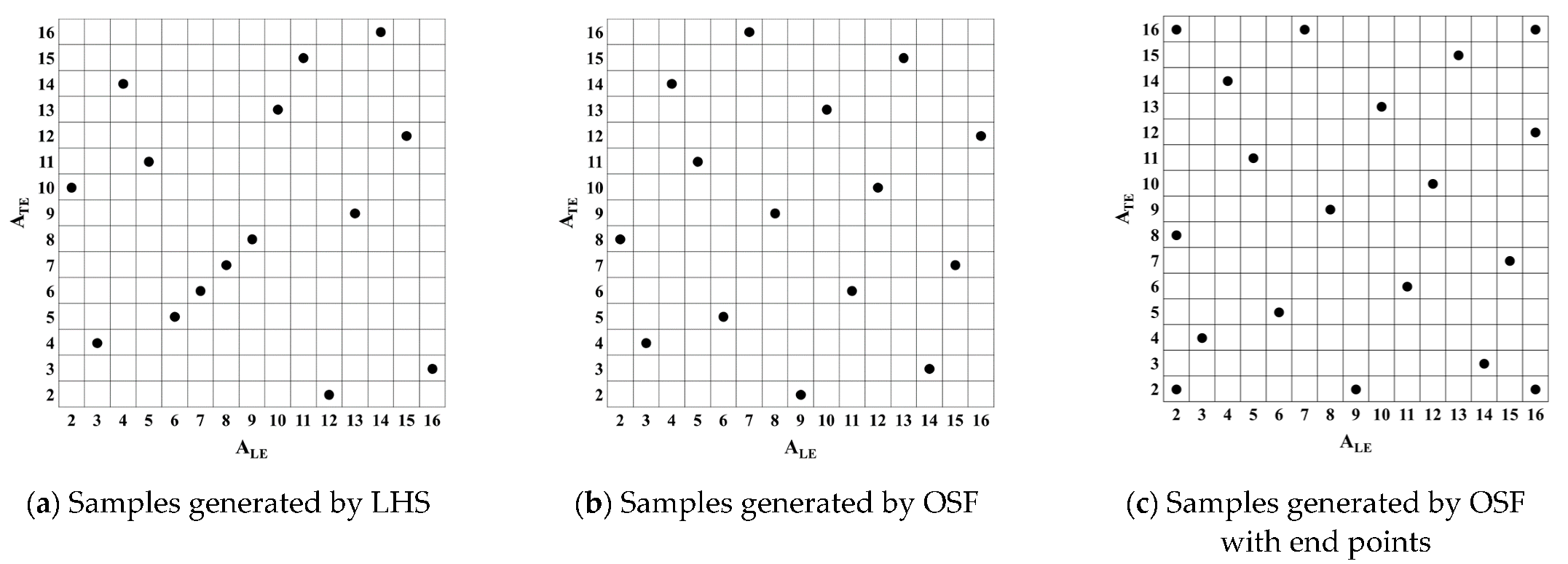
Design of experiments (DOE) was conducted to investigate the effect of the variation of the elliptic aspect ratios of the blade leading and trailing edge (see Figure 4) on the performance of the hydro turbine. The DOE is a method of logically analyzing the results, using statistical theory by efficiently placing experimental conditions, rather than performing experiments on all design variables within the range of the experimental area of interest. Unlike physical experiments, there is no random error in computational experiments; therefore, it is known that sampling methods which uniformly fill the experimental areas, the so-called “space-filling” concept, are appropriate [41]. Latin hypercube sampling (LHS) is a method of dividing each of the dimensions in the experimental design into regions with equal levels and extracting one sample from each region [42]. It is known to be a suitable sampling method for computational experiments, because it satisfies the concept of space-filling. One disadvantage of LHS is that it places samples randomly in the experimental area, hence it is likely that the distributed samples will be uneven. Optimal space-filling (OSF) is a sampling method based on LHS, but by maximizing the minimum distance between the points, it provides a more uniform distribution within the design space [43]. In this study, the design variables were sampled using OSF, and Figure 5b shows the distribution of extracted design variables within the experimental area. However, OSF does not include endpoints in the experimental area, which has the disadvantage of being less accurate at endpoints. Therefore, the samples for DOE added endpoints to the samples from OSF as shown in Figure 5c. The ranges of the elliptic aspect ratios of the blade leading and trailing edge were set to 2–16.

3.2. Response Surface

To analyze the effect of each design variable on the performance, genetic aggregation response surface (GARS) was used to generate the response surface. GARS is a method of adopting the best response surface using the weighted aggregation of several other metamodels. It can be expressed as Equation (6):
y ^ e n s ( x ) = i N M w i ( x ) y ^ i ( x )
where y ^ e n s is the prediction of the ensemble, N M is the number of metamodels used, w i is the weight factor for the i-th metamodel, and y ^ i is the prediction of the i-th metamodel. It corrects the deviation by K-fold cross-validation [44]. The commercial code, ANSYS DesignXplorer, was used to implement GARS.

3.3. Optimization

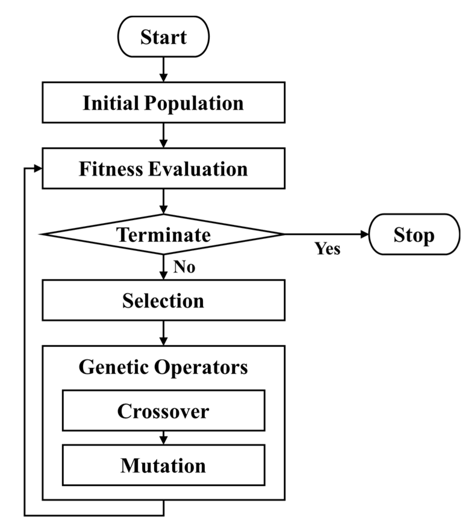
Genetic algorithm (GA) was used to find the optimal point of the elliptic aspect ratios of the blade leading and trailing edge having the highest efficiency in the design range. GA is an algorithm that mimics the evolution of individuals as they adapt to the natural environment. It is suitable for optimization as it is likely to choose the optimal solution as they evolve. It selects a superior population from a random population and uses the crossover and mutation operators to create the next generation. This process is repeated until the fitness is satisfied [45]. Figure 6 illustrates a general flowchart of GA procedures. To implement the GA, the commercial code, ANSYS DesignXplorer, was utilized.

4. Results and Discussion

4.1. Sensitivity Analysis

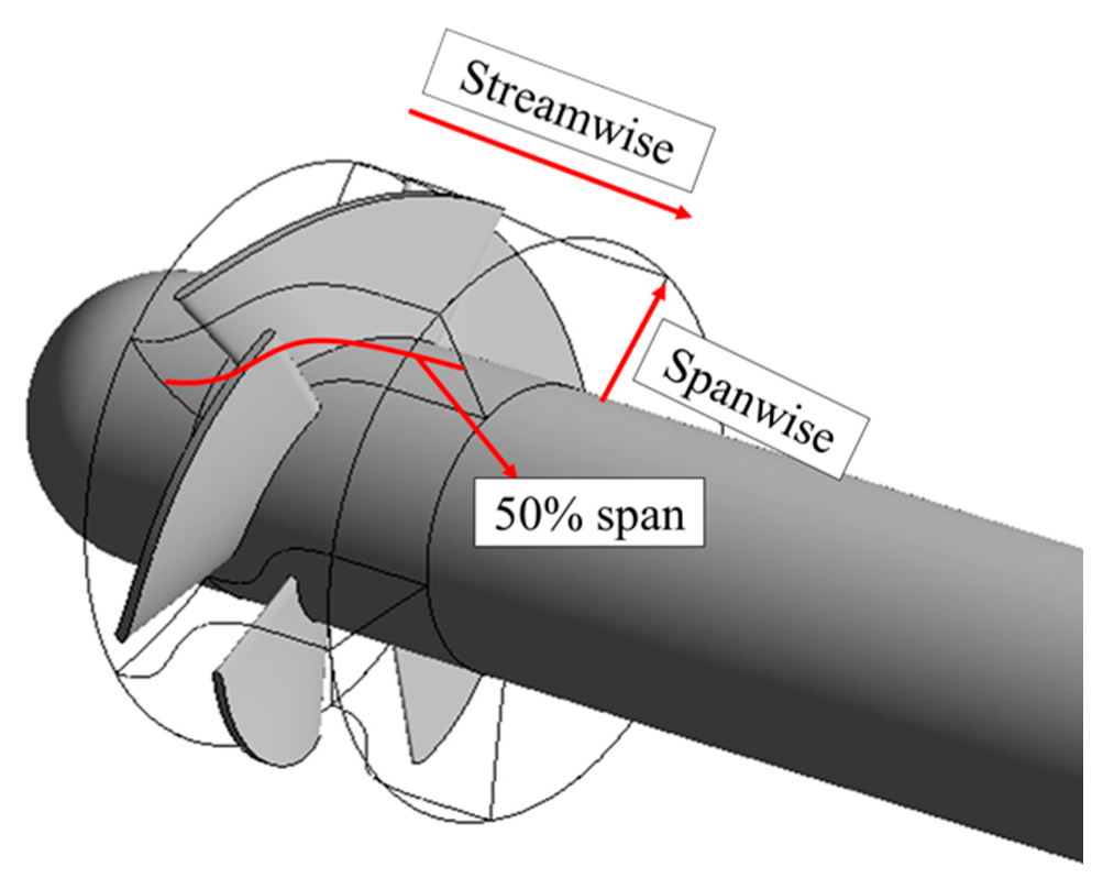
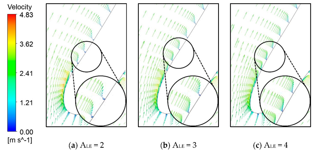
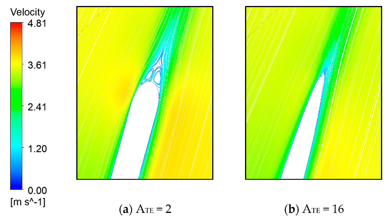
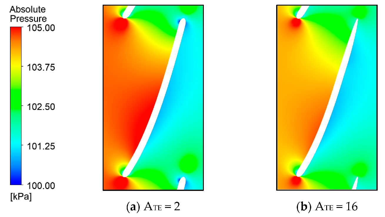
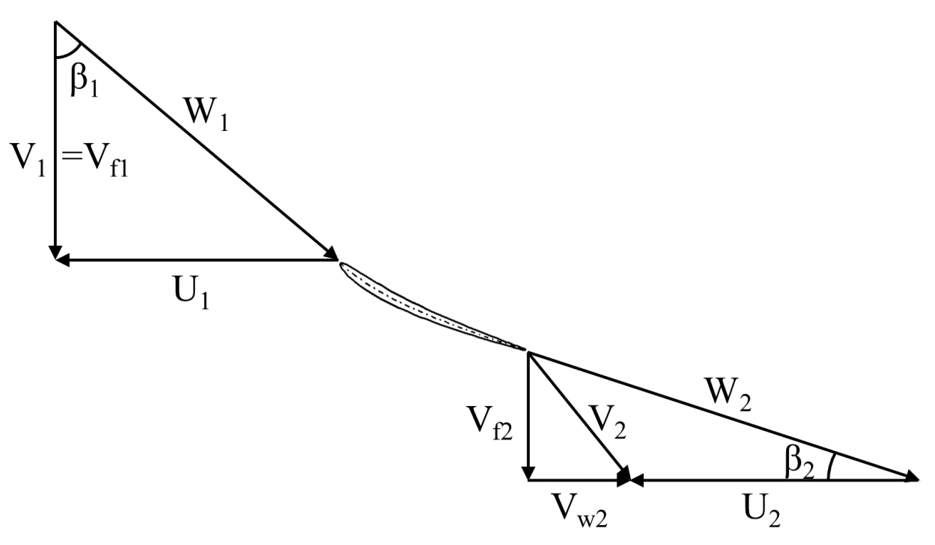
Figure 7 shows the generated response surface for sensitivity analysis of the design variables. The x-axis and y-axis represent the elliptic aspect ratios of the leading and trailing edge of the blade, respectively, while the z-axis indicates the power, head, and efficiency from left to right. Between the elliptic aspect ratios of the leading and trailing edge of the blade, the more sensitive design variable in terms of performance is the latter, and there is a tendency that as the blade edges sharpen, the power and head decrease. In addition, the response surface in the region of 2–4 for ALE is rather steep, especially for the efficiency. This can be considered for several reasons. Here, the figures used in the explanation are represented at 50% span which is the middle of the hub and shroud (see Figure 8). First, for the blunt leading edge (particularly ALE = 2 or 3), the flow separation occurs due to the strong adverse pressure (see Figure 9). This is because of the drastic change of curvature radius. Furthermore, the sharper the trailing edge, the more the flow separation is delayed (see Figure 10), and the lower the pressure on the pressure side (see Figure 11 and Figure 12). In addition, in the case of the leading edge, drastic variation of the pressure is inevitably formed due to the stagnation point, regardless of the change of the leading edge shape of the blade (see Figure 13). The sharper the leading edge, the greater the tendency of the drastic pressure fluctuation on the suction side to be resolved, but the more insignificant the overall pressure difference between the pressure and suction sides becomes (see Figure 14). Moreover, the results can be considered using the velocity triangle at the inlet and outlet of the blade. The water flows in a straight direction until just before the runner entrance, due to the absence of a guide vane. Figure 15 shows that the absolute velocity and blade linear velocity are perpendicular at the leading edge. Equation (7) indicates Euler’s turbine equation, which enables calculation of the theoretical turbine output based on Newton’s second law of motion [46]:
P = ρ Q ( V 1 U 1 V 2 U 2 )
In the equation, V 1 U 1 , corresponding to the velocity component at the leading edge, has the value of 0, due to the orthogonality. As a result, the variation of the curvature of the leading edge configuration does not significantly affect the performance.
For these reasons, there are many studies focused on blade trailing edge rather than leading edge to improve blade performance. For a case in point, there is a study that modified the blunt trailing edge thickness of the airfoil to improve the aerodynamic performance of a wind turbine [47]. In addition, the blade trailing edge profile also has a significant effect on pump performance, and there is a case where pressure pulsations in a centrifugal pump were reduced through modification of the blade trailing edge profile [48].

4.2. Results of the Modified Model

The elliptic aspect ratios of the blade leading and trailing edge of the reference model are two. The most efficient points of the elliptic aspect ratios of the blade leading and trailing edge derived through the GA were calculated as 5.5 and 16, respectively. To verify the predicted point, numerical analysis was conducted with the calculated elliptic aspect ratios of the blade edges. Table 4 specifies the comparison results, and the relative errors are less than 1%; thus we can conclude that the prediction is verified. At this time, the power and head decrease by about 8% and 11%, respectively, compared to the reference model, and the efficiency increases by 2.16%.

4.3. Application of the NACA Airfoil

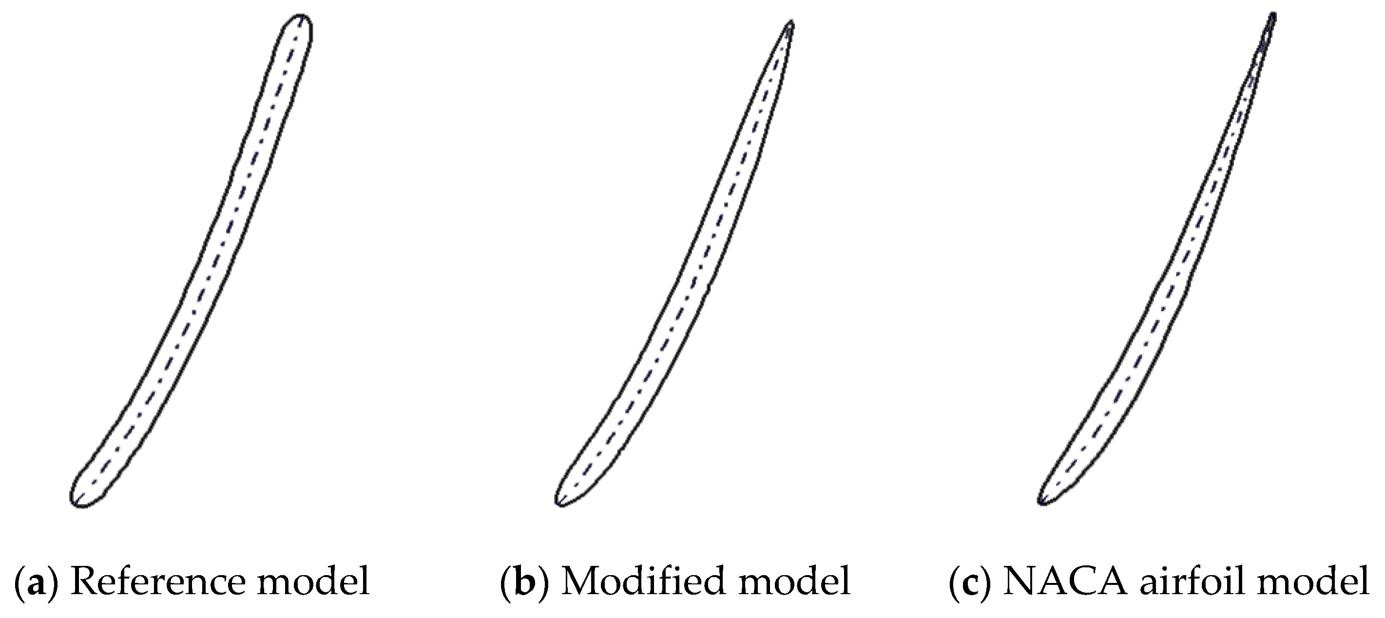
An airfoil refers to the cross-sectional shape of an airplane’s wings. In 1929, the National Advisory Committee for Aeronautics (NACA) studied a series of airfoils, and systematically standardized them to be suitable for specific conditions [49]. The NACA airfoils play a role in improving the aerodynamic performance of the airplane, and if applied to the hydro turbine blade, may be expected to stabilize the flow passing through the runner, and improve the performance of the hydro turbine. In particular, the maximum thickness of the NACA 4-digit series airfoil models is located at 30% of the chord from the leading edge [50]. This configuration has a similarity to the results previously derived from the optimization of the blade leading and trailing edge elliptic aspect ratios. Taking these into consideration, a NACA 4-digit series airfoil model was applied to the blade profile of the micro tubular propeller turbine, and numerical analysis was conducted to analyze and compare the performance with the reference model. The blade angle was set to be identical to the reference model. Based on the camber line, the NACA 0004 to the hub face and NACA 0006 to the blade tip were applied to keep the maximum thickness of 1.7 mm, which is the same as the reference model. Figure 16 compares the blade cross-sectional shape on the hub face of the reference, modified, and NACA airfoil model, while Table 5 describes the results of the numerical analysis.
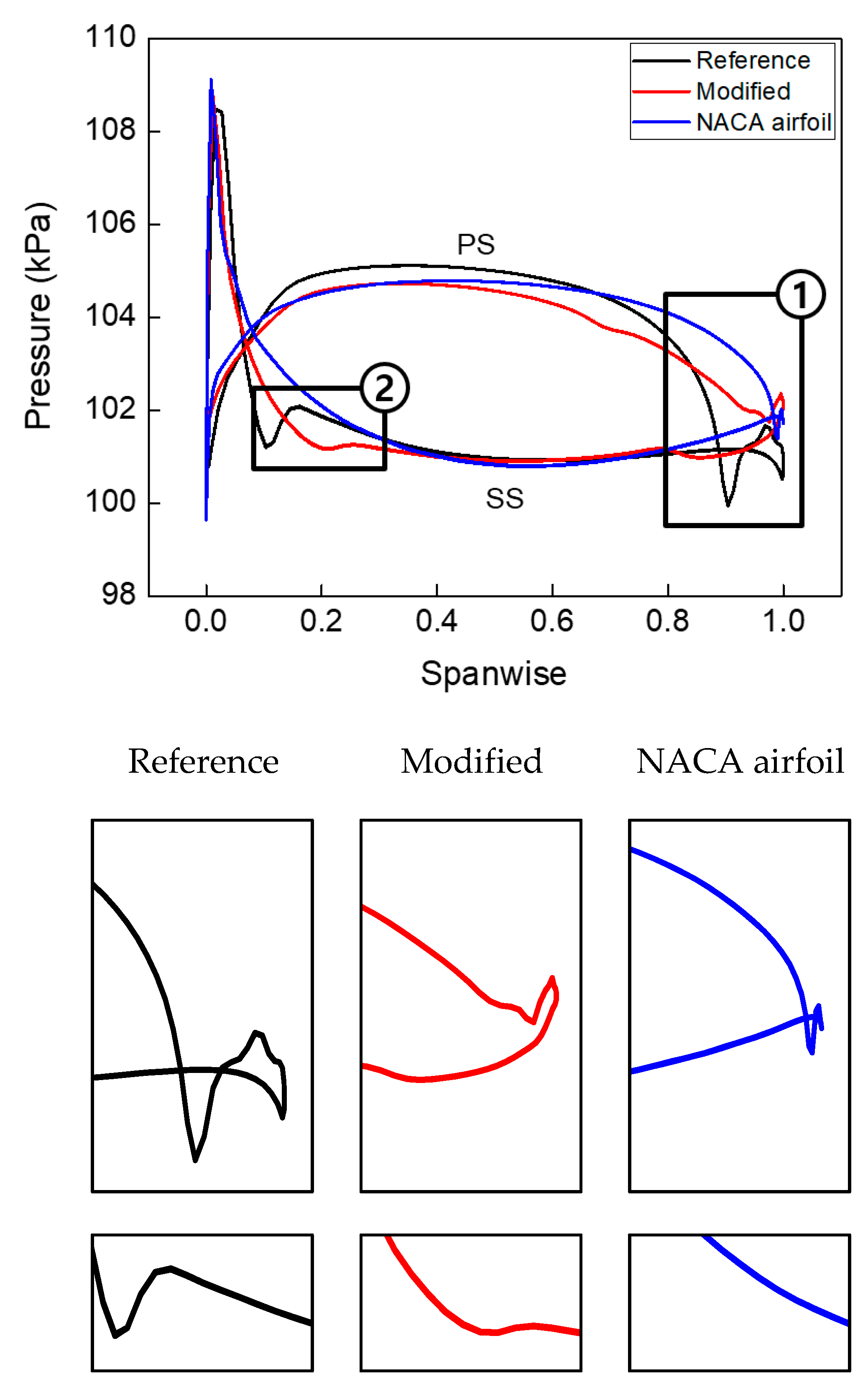
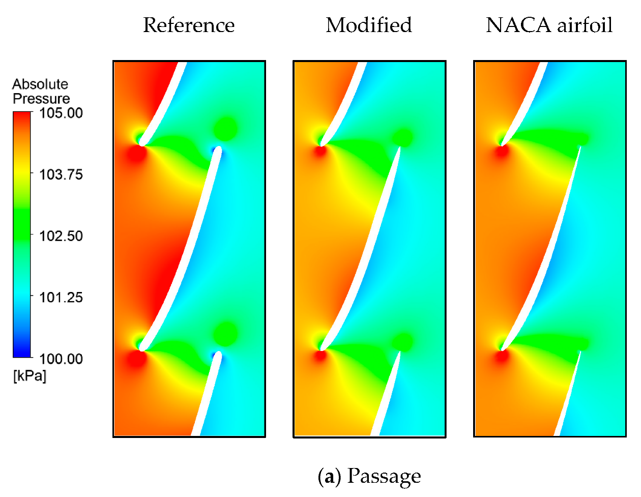
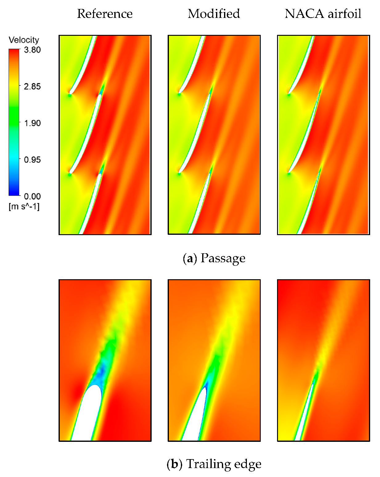
Figure 17 shows the pressure variation along the blade surface. The pressure fluctuation at the trailing edge is resolved for the modified model and the NACA airfoil model, compared to the reference model. In addition, the pressure variation line on the blade surface is the smoothest for the NACA airfoil model, so we can assume that the flow becomes stable. Furthermore, the flow becoming stable can also be determined through Figure 18, which shows the pressure distribution in the flow at the runner. In addition, as can be seen in the velocity distribution shown in Figure 19, the wake generated at the trailing edge is the weakest for the NACA airfoil, which results in the least influence from the wake.
The cases of applying a NACA airfoil to the hydro turbine can support the results of this study. For instance, a NACA airfoil is applied to the guide vane in the Francis turbine [51,52], and also to the runner blade [53]. In addition, there are examples of applications to the axis tidal turbine [54,55].

5. Conclusions

In this study, a micro tubular propeller turbine with a simple configuration and easy maintenance was selected for micro hydropower in pipes. The effect of the blade leading and trailing edge configuration on the performance of the hydro turbine was analyzed numerically. The variation of the performance depending on the design variables was efficiently studied through DOE and GARS, and it turned out that the trailing edge configuration is more sensitive to the performance. This is because the flow separation delays at the sharper trailing edge, and the sudden change of pressure does not disappear even if the leading edge configuration has changed due to the inevitably formed stagnation point. To improve the performance of the hydro turbine, a NACA airfoil was applied to the blade of hydro turbine, and it was effective in stabilizing the flow. It results in 2.44% increased efficiency compared to the reference model.

Author Contributions

Conceptualization, S.J.; methodology, S.J.; software, S.J.; validation, S.J. and Y.-W.J.; formal analysis, S.J.; investigation, S.J.; resources, Y.-J.K.; data curation, S.J.; writing—original draft preparation, S.J.; writing—review and editing, S.J. and Y.-J.K.; visualization, S.J.; supervision, Y.-J.K.; project administration, Y.-J.K.; funding acquisition, Y.-W.J. and Y.-J.K. All authors have read and agreed to the published version of the manuscript.

Funding

This research was funded by the Korea Midland Power Co., Ltd., grant number 2019-field-03.

Conflicts of Interest

The authors declare no conflict of interest.

Nomenclature

DpPipe diameter [mm]
DbBlade diameter [mm]
DhHub diameter [mm]
LhFront hub length [mm]
LbBlade length [mm]
tbBlade thickness [mm]
tcTip clearance [mm]
β1Hub leading edge angle [°]
β2Hub trailing edge angle [°]
β3Tip leading edge angle [°]
β4Tip trailing edge angle [°]
TTorque [N·m]
NRotational speed [rad/s]
P Power [W]
Δ p Pressure difference between runner inlet and outlet [Pa]
H Head [m]
ρ Working fluid density [kg/m3]
g Gravitational acceleration [m/s2]
Q Flow rate [m3/s]
η Hydraulic efficiency [%]
μ Dynamic viscosity [Pa·s]
u τ Wall shear velocity [m/s]
τ w Wall shear stress [Pa]
y Wall distance [m]
y + Y-plus
u Velocity [m/s] (in 2.5 Governing Equations)
τ i j Stress tensor [Pa]
ρ u i u j ¯ Reynolds stresses [Pa]
δ i j Kronecker delta
μ t Turbulent dynamic viscosity [Pa·s]
k Turbulence kinetic energy [m2/s2]
r1Blade leading and trailing edge semi-minor axis length [mm]
r2Blade leading and trailing edge semi-major axis length [mm]
ALEElliptic aspect ratio at leading edge
ATEElliptic aspect ratio at trailing edge
y ^ e n s Prediction of the ensemble
N M Number of metamodels used
w i Weight factor for i-th metamodel
y ^ i Prediction of i-th metamodel
VAbsolute velocity in velocity triangle [m/s]
VfFlow velocity in velocity triangle (Vertical component of absolute velocity) [m/s]
VrWhirl velocity in velocity triangle (Horizontal component of absolute velocity) [m/s]
UBlade velocity in velocity triangle [m/s]
WRelative velocity in velocity triangle [m/s]

References

  1. UNFCCC. The Paris Agreement. Available online: https://unfccc.int/process-and-meetings/the-paris-agreement/the-paris-agreement (accessed on 2 February 2021).
  2. Center for Climate and Energy Solutions. Global Emissions. Available online: https://www.c2es.org/content/international-emissions/ (accessed on 3 February 2021).
  3. Climatewatch. Historical GHG Emissions. Available online: https://www.climatewatchdata.org/ghg-emissions?breakBy=sector&chartType=percentage&end_year=2017&gases=all-ghg&start_year=1990 (accessed on 3 February 2021).
  4. Our World in Data. Sector by Sector: Where Do Global Greenhouse Gas Emissions Come from? Available online: https://ourworldindata.org/ghg-emissions-by-sector (accessed on 3 February 2021).
  5. REN21. Renewables 2020 Global Status Report; REN21 Secretariat: Paris, France, 2020; p. 48. Available online: https://www.ren21.net/wp-content/uploads/2019/05/gsr_2020_full_report_en.pdf (accessed on 21 April 2021).
  6. Panwar, N.L.; Kaushik, S.C.; Kothari, S. Role of renewable energy sources in environmental protection: A review. Renew. Sustain. Energy Rev. 2011, 15, 1513–1524. [Google Scholar] [CrossRef]
  7. Okot, D.K. Review of small hydropower technology. Renew. Sustain. Energy Rev. 2013, 26, 515–520. [Google Scholar] [CrossRef]
  8. IRENA. Renewable Energy Statistics 2020; The International Renewable Energy Agency: Abu Dhabi, United Arab Emirates, 2020; pp. 1–15. [Google Scholar]
  9. Hoes, O.A.; Meijer, L.J.; Van Der Ent, R.J.; Van De Giesen, N.C. Systematic high-resolution assessment of global hydropower potential. PLoS ONE 2017, 12, e0171844. [Google Scholar] [CrossRef]
  10. Nasir, B.A. Design considerations of micro-hydro-electric power plant. Energy Procedia 2014, 50, 19–29. [Google Scholar] [CrossRef]
  11. Jawahar, C.P.; Michael, P.A. A review on turbines for micro hydro power plant. Renew. Sustain. Energy Rev. 2017, 72, 882–889. [Google Scholar] [CrossRef]
  12. Elbatran, A.H.; Yaakob, O.B.; Ahmed, Y.M.; Shabara, H.M. Operation, performance and economic analysis of low head micro-hydropower turbines for rural and remote areas: A review. Renew. Sustain. Energy Rev. 2015, 43, 40–50. [Google Scholar] [CrossRef]
  13. Davis, S. Microhydro: Clean Power from Water; New Society Publishers: Gabriola Island, BC, Canada, 2003; pp. 8–9. [Google Scholar]
  14. Casini, M. Harvesting energy from in-pipe hydro systems at urban and building scale. Int. J. Smart Grid Clean Energy 2015, 4, 316–327. [Google Scholar] [CrossRef] [Green Version]
  15. Krzemianowski, Z.; Steller, J. High specific speed francis turbine for small hydro purposes-design methodology based on solving the inverse problem in fluid mechanics and the cavitation test experience. Renew. Energy 2021, 169, 1210–1228. [Google Scholar] [CrossRef]
  16. Gohil, P.P.; Saini, R. Effect of temperature, suction head and flow velocity on cavitation in a Francis turbine of small hydro power plant. Energy 2015, 93, 613–624. [Google Scholar] [CrossRef]
  17. Daniels, S.; Rahat, A.; Tabor, G.; Fieldsend, J.; Everson, R. Shape optimisation of the sharp-heeled Kaplan draft tube: Performance evaluation using computational fluid dynamics. Renew. Energy 2020, 160, 112–126. [Google Scholar] [CrossRef]
  18. Chen, H.; Zhou, D.; Zheng, Y.; Jiang, S.; Yu, A.; Guo, Y. Load rejection transient process simulation of a Kaplan turbine model by co-adjusting guide vanes and runner blades. Energies 2018, 11, 3354. [Google Scholar] [CrossRef] [Green Version]
  19. Lugauer, F.J.; Kainz, J.; Gaderer, M. Techno-economic efficiency analysis of various operating strategies for micro-hydro storage using a pump as a turbine. Energies 2021, 14, 425. [Google Scholar] [CrossRef]
  20. Morabito, A.; e Silva, G.D.O.; Hendrick, P. Deriaz pump-turbine for pumped hydro energy storage and micro applications. J. Energy Storage 2019, 24, 100788. [Google Scholar] [CrossRef]
  21. Lin, T.; Zhu, Z.; Li, X.; Li, J.; Lin, Y. Theoretical, experimental, and numerical methods to predict the best efficiency point of centrifugal pump as turbine. Renew. Energy 2021, 168, 31–44. [Google Scholar] [CrossRef]
  22. Chen, J.; Yang, H.X.; Liu, C.P.; Lau, C.H.; Lo, M. A novel vertical axis water turbine for power generation from water pipelines. Energy 2013, 54, 184–193. [Google Scholar] [CrossRef]
  23. Payambarpour, S.A.; Najafi, A.F.; Magagnato, F. Investigation of deflector geometry and turbine aspect ratio effect on 3D modified in-pipe hydro Savonius turbine: Parametric study. Renew. Energy 2020, 148, 44–59. [Google Scholar] [CrossRef]
  24. Team, Purdue ECT. LUCIDPIPETM power system. ECT Fact Sheets 2016, 224. Available online: https://docs.lib.purdue.edu/ectfs/224/ (accessed on 15 June 2021).
  25. Yeo, H.; Seok, W.; Shin, S.; Huh, Y.C.; Jung, B.C.; Myung, C.-S.; Rhee, S.H. Computational analysis of the performance of a vertical axis turbine in a water pipe. Energies 2019, 12, 3998. [Google Scholar] [CrossRef] [Green Version]
  26. Hydrocoil Power, Inc. Available online: http://www.hydrocoil.com (accessed on 8 February 2021).
  27. Sinagra, M.; Aricò, C.; Tucciarelli, T.; Morreale, G. Experimental and numerical analysis of a backpressure Banki inline turbine for pressure regulation and energy production. Renew. Energy 2020, 149, 980–986. [Google Scholar] [CrossRef]
  28. Nan, D.; Shigemitsu, T.; Zhao, S.; Ikebuchi, T.; Takeshima, Y. Study on performance of contra-rotating small hydro-turbine with thinner blade and longer front hub. Renew. Energy 2018, 117, 184–192. [Google Scholar] [CrossRef]
  29. Vagnoni, E.; Andolfatto, L.; Richard, S.; Münch-Alligné, C.; Avellan, F. Hydraulic performance evaluation of a micro-turbine with counter rotating runners by experimental investigation and numerical simulation. Renew. Energy 2018, 126, 943–953. [Google Scholar] [CrossRef] [Green Version]
  30. Chen, C.W. Handbook of Hydraulic Turbines and Pump Turbines; Auris Reference Ltd.: London, UK, 2014; p. 525. [Google Scholar]
  31. Duquesne, P.; Maciel, Y.; Deschênes, C. Investigation of flow separation in a diffuser of a bulb turbine. J. Fluids Eng. 2016, 138, 011102. [Google Scholar] [CrossRef]
  32. Li, Y.; Song, G.; Yan, Y. Transient hydrodynamic analysis of the transition process of bulb hydraulic turbine. Adv. Eng. Softw. 2015, 90, 152–158. [Google Scholar] [CrossRef]
  33. Chen, H.; Zhou, D.; Kan, K.; Xu, H.; Zheng, Y.; Binama, M.; Xu, Z.; Feng, J. Experimental investigation of a model bulb turbine under steady state and load rejection process. Renew. Energy 2021, 169, 254–265. [Google Scholar] [CrossRef]
  34. Shandilya, S.; Shelar, S.P.; Das, S.P.; Chatterjee, D.; Saini, R. Performance evaluation of a bulb turbine designed for ultra-low head applications. J. Phys. Conf. Ser. 2019, 1276, 012024. [Google Scholar] [CrossRef]
  35. Samora, I.; Hasmatuchi, V.; Münch-Alligné, C.; Franca, M.J.; Schleiss, A.J.; Ramos, H.M. Experimental characterization of a five blade tubular propeller turbine for pipe inline installation. Renew. Energy 2016, 95, 356–366. [Google Scholar] [CrossRef]
  36. Dixon, S.L.; Hall, C.A. Fluid Mechanics and Thermodynamics of Turbomachinery, 7th ed.; Butterworth-Heinemann: Oxford, UK, 2014; pp. 22–25. [Google Scholar]
  37. Adanta, D.; Budiarso, B.; Siswantara, A.I. Assessment of turbulence modelling for numerical simulations into pico hydro turbine. J. Adv. Res. Fluid Mech. Therm. Sci. 2018, 46, 21–31. [Google Scholar]
  38. Warjito, W.; Nasution, S.B.; Syahputra, M.F.; Budiarso, B.; Adanta, D. Study of turbulence model for performance and flow field prediction of pico hydro types propeller turbine. CFD Lett. 2020, 12, 26–34. [Google Scholar] [CrossRef]
  39. ANSYS. ANSYS CFX-Solver Theory Guide; ANSYS Inc.: Canonsburg, PA, USA, 2020; p. 80. [Google Scholar]
  40. Moukalled, F.; Mangani, L.; Darwish, M. The Finite Volume Method in Computational Fluid Dynamics; Springer: Cham, Switzerland, 2016. [Google Scholar]
  41. Garud, S.S.; Karimi, I.A.; Kraft, M. Design of computer experiments: A review. Comput. Chem. Eng. 2017, 106, 71–95. [Google Scholar] [CrossRef]
  42. Viana, F.A. A tutorial on Latin hypercube design of experiments. Qual. Reliab. Eng. Int. 2016, 32, 1975–1985. [Google Scholar] [CrossRef]
  43. Joseph, V.R. Space-filling designs for computer experiments: A review. Qual. Eng. 2016, 28, 28–35. [Google Scholar] [CrossRef]
  44. Ben Salem, M.; Roustant, O.; Gamboa, F.; Tomaso, L. Universal prediction distribution for surrogate models. SIAM/ASA J. Uncertain. Quantif. 2017, 5, 1086–1109. [Google Scholar] [CrossRef] [Green Version]
  45. Mirjalili, S. Genetic Algorithm. In Evolutionary Algorithms and Neural Networks; Springer: Cham, Switzerland, 2019; pp. 43–55. [Google Scholar]
  46. Sultanian, B. Logan’s Turbomachinery: Flowpath Design and Performance Fundamentals, 3rd ed.; CRC Press: Boca Raton, FL, USA, 2019; pp. 22–23. [Google Scholar]
  47. Zhang, X.; Li, W.; Liu, H. Numerical simulation of the effect of relative thickness on aerodynamic performance improvement of asymmetrical blunt trailing-edge modification. Renew. Energy 2015, 80, 489–497. [Google Scholar] [CrossRef]
  48. Gao, B.; Zhang, N.; Li, Z.; Ni, D.; Yang, M. Influence of the blade trailing edge profile on the performance and unsteady pressure pulsations in a low specific speed centrifugal pump. J. Fluids Eng. 2016, 138, 051106. [Google Scholar] [CrossRef]
  49. NASA. NACA Airfoils. Available online: https://www.nasa.gov/image-feature/langley/100/naca-airfoils (accessed on 11 June 2021).
  50. Bramantya, M.A.; Ginting, R.R.R. Study of the effect of 4-digit NACA variation on airfoil performance using computation fluid dynamics. AIP Conf. Proc. 2020, 2248, 020002. [Google Scholar]
  51. Thapa, B.S.; Dahlhaug, O.G.; Thapa, B. Flow measurements around guide vanes of francis turbine: A piv approach. Renew. Energy 2018, 126, 177–188. [Google Scholar] [CrossRef]
  52. Chitrakar, S.; Thapa, B.S.; Dahlhaug, O.G.; Neopane, H.P. Numerical and experimental study of the leakage flow in guide vanes with different hydrofoils. J. Comput. Des. Eng. 2017, 4, 218–230. [Google Scholar] [CrossRef]
  53. Jeon, J.-H.; Byeon, S.-S.; Kim, Y.-J. Numerical study on the flow characteristics of the Francis turbine with various blade profiles. In Proceedings of the ASME 2013 Fluids Engineering Division Summer Meeting, Incline Village, NV, USA, 7–11 July 2013. [Google Scholar]
  54. Goundar, J.N.; Ahmed, M.R. Design of a horizontal axis tidal current turbine. Appl. Energy 2013, 111, 161–174. [Google Scholar] [CrossRef]
  55. Mohammadi, S.; Hassanalian, M.; Arionfard, H.; Bakhtiyarov, S. Optimal design of hydrokinetic turbine for low-speed water flow in golden gate strait. Renew. Energy 2020, 150, 147–155. [Google Scholar] [CrossRef]
Figure 1. Schematic of the micro tubular propeller turbine model system.
Applsci 11 05596 g001
Figure 2. Runner model.
Applsci 11 05596 g002
Figure 3. Grid dependency test (ac).
Applsci 11 05596 g003
Figure 4. Elliptic aspect ratio of the blade edge.
Applsci 11 05596 g004
Figure 5. Comparison of sample distribution within the design area (ac).
Applsci 11 05596 g005
Figure 6. Process of genetic algorithm.
Applsci 11 05596 g006
Figure 7. Response surface (ac).
Applsci 11 05596 g007
Figure 8. Location of 50% span.
Applsci 11 05596 g008
Figure 9. Velocity vector distributions at the leading edge at 50% span of the different elliptic aspect ratios of the leading edge (ac).
Applsci 11 05596 g009
Figure 10. Streamlines at 50% span of the different elliptic aspect ratios of the trailing edge (a,b).
Applsci 11 05596 g010
Figure 11. Pressure distribution at 50% span of the different elliptic aspect ratios of the trailing edge (a,b).
Applsci 11 05596 g011
Figure 12. Blade loading at 50% span of the different elliptic aspect ratios of the trailing edge.
Applsci 11 05596 g012
Figure 13. Stagnation point at 50% span of the different elliptic aspect ratios of the leading edge (a,b).
Applsci 11 05596 g013
Figure 14. Blade loading at 50% span of the different elliptic aspect ratios of the leading edge.
Applsci 11 05596 g014
Figure 15. Velocity triangle at the leading and trailing edge of the blade.
Applsci 11 05596 g015
Figure 16. Comparison of the cross-sectional configurations of the blade on the hub (ac).
Applsci 11 05596 g016
Figure 17. Blade loading at 50% span of the different models.
Applsci 11 05596 g017
Figure 18. Pressure distribution contours at 50% span of the different models (ac).
Applsci 11 05596 g018aApplsci 11 05596 g018b
Figure 19. Velocity distribution contours at 50% span of the different models (a,b).
Applsci 11 05596 g019
Table 1. Specification of the micro tubular propeller turbine.
ClassificationValue
Pipe diameter, Dp [mm]85
Blade diameter, Db [mm]84.8
Hub diameter, Dh [mm]42.5
Front hub length, Lh [mm]23.5
Blade length, Lb [mm]18.5
Blade thickness, tb [mm]1.7
Tip clearance, tc [mm]0.1
Hub leading edge angle, β1 [°]42.5
Hub trailing edge angle, β2 [°]18
Tip leading edge angle, β3 [°]34.5
Tip trailing edge angle, β4 [°]13.5
Number of blades [-]5
Table 2. Boundary conditions applied in this study.
ClassificationValue
Analysis stateSteady state
Interface modelFrozen rotor
Turbulence modelSST
Working fluidWater at 25 °C
Inlet conditionFlow rate (15.95 m3/h)
Outlet conditionStatic pressure (1 atm)
Rotational speed750 rpm
Table 3. Comparison of the steady state, unsteady state and reference experimental results.
Power [W]Head [m]Efficiency [%]
Steady9.4230.35062.13
Unsteady9.3460.34861.95
Reference9.3930.3463.75
Table 4. Comparative results of prediction and verification.
ALEATEPower [W]Head [m]Efficiency [%]
Prediction5.5168.7020.31364.29
Verification8.6620.31164.27
Error [%]--0.460.550.03
Table 5. Comparison of the reference, modified, and NACA airfoil model results.
Power [W]Head [m]Efficiency [%]
Reference model9.4230.35062.13
Modified model8.6620.31164.27
NACA airfoil model9.1930.32964.57
Publisher’s Note: MDPI stays neutral with regard to jurisdictional claims in published maps and institutional affiliations.