Article

Modeling of Tunneling Total Loads Based on Symbolic Regression Algorithm

School of Mechanical Engineering, Tianjin University, Tianjin 300350, China
*
Author to whom correspondence should be addressed.
Appl. Sci. 2021, 11(12), 5671; https://doi.org/10.3390/app11125671
Submission received: 28 April 2021 / Revised: 4 June 2021 / Accepted: 15 June 2021 / Published: 18 June 2021
(This article belongs to the Section Mechanical Engineering)

Abstract

:
The tunneling total load is one of the core control parameters for safe and efficient construction using tunneling machines. However, because the tunneling process involves complex coupling relationships between the equipment and the local geology, theoretical derivation is difficult. The development of tunneling data detection and acquisition technology has led to extensive load modeling based on data analysis and machine learning. However, it is difficult to obtain an explicit interpretable model that satisfies certain physical rules. In this paper, a modeling method based on symbolic regression is proposed. The method mainly includes three modules: construction of π quantities, feature selection, and model training. Through dimensional analysis, the π quantities are constructed so as to impose physical constraints on the training process. Feature selection based on a nonlinear random forest model is used to improve the modeling efficiency. Finally, an explicit nonlinear load model is obtained using symbolic regression, which satisfies the basic equilibrium theory of mechanics and the dimensional rules of physics. The proposed approach is compared with general linear regression and an artificial neural network. The results show that the proposed method produces a load model that is interpretable and accurate, providing an excellent reference for construction excavation.

1. Introduction

In recent years, tunnel boring machines (TBMs) have been widely used in the construction of urban subways and tunnels through mountains [1,2,3,4,5]. TBMs are a kind of large-scale engineering equipment working under considerable loads, and often operate in complex and changeable construction environments [6,7]. Safe and efficient tunneling is vital for the equipment and the stability of the ground environment [8]. The TBM construction process mainly involves the interaction between the machine and the local geology, in which the tunneling total load, mainly composed of the total thrust and the total torque, is one of the core control parameters [9,10]. During the construction process, the equipment must overcome resistance to move forward under the action of the total thrust, and the cutter installed on the cutter head penetrates into the stratum and remains spinning under the action of the total torque. Therefore, modeling and predicting the tunneling total loads is of great significance.
Modeling the tunneling load has long been a concern in this field. The classic approaches are Krause’s empirical formula model for shield tunneling in soft soil [11] and the Colorado School of Mines (CSM) model for shield tunneling in hard rock [12,13]. Krause’s empirical formula reflects the basic mechanical equilibrium information through the power relationship between the load and the equipment diameter, with other influencing factors such as geology covered by empirical coefficients. This empirical formula provides a relatively broad range of predicted values, but the model is simple and easy to operate, and so it has been widely used. The CSM model is based on force calculations and statistical data fitting, mainly from indoor linear cutting experiments [14,15]. To obtain load models that are more suitable for actual complex construction environments, many scholars have carried out further related studies. Analytical methods can be divided into two categories: modeling based on theoretical derivation and modeling based on data analysis. Modeling based on theoretical derivation includes an improved version of Krause’s empirical formula, in which the composition of the cutter head torque is analyzed for composite geology [10]. In Ref. [16], considering the structure of the cutter head, the cutting principle, and the interaction between the cutter head and soil, the composition of the cutter head torque is divided into eight parts that are calculated to obtain the final load model. In Ref. [17], the composition of the total thrust force is analyzed and divided into frontal resistance, frictional resistance, penetration resistance, segmental ring friction, and auxiliary facility resistance. The thrust model for a sandy geology is then obtained. In Refs. [18,19], the coupling relationship between the cutter head and the local geology is analyzed and theoretical load models are established by considering the influence of three key factors on the load, namely the geological conditions, operating state, and equipment structure. However, the complexity of tunneling construction means that load models constructed based on theoretical analysis are often complicated and have limited consideration of the actual geological conditions; for example, the classic CSM model does not consider the influence of rock mass density and cohesion [2]. Therefore, many researchers have attempted to build load models through data analysis methods. There are two types of load modeling methods based on data analysis: traditional mathematical statistical methods and machine learning algorithms. The traditional mathematical statistical methods include a cutter head torque model established with multivariate statistical analysis based on orthogonal experiments [20]. In Ref. [21], an empirical estimation model of the cutter head load is established by linear regression based on data from improved traditional cutting experiments. In Ref. [22], based on in situ engineering data, the cutter torque is modeled by statistical analysis of the function relationship among parameters, and the coefficient is identified by multiple linear regression. In Ref. [9], data from a number of TBMs are statistically analyzed, and an empirical model of the relationship between the tunneling loads and the diameter of the cutter head is obtained. In Ref. [23], previous studies on data analysis methods are reviewed, and polynomial exponential regression is used to predict the TBM loads. In this kind of regression modeling, it is difficult to determine the nonlinear relationship among the parameters. This is often determined by analyzing the correlation among different elementary functions, but this may lead to an insufficient description of the physical constraint relationship among the parameters. With the increasing abundance of real-time monitoring data and the rapid development of machine learning technology, machine learning modeling based on engineering data is increasing, laying the foundation for determining the coupling relationship between parameters and building load models that fully reflect the nonlinear mapping relationship. Several researchers have modeled tunneling loads based on machine learning algorithms. In Ref. [24], the long short-term memory algorithm is applied to predict the total thrust and cutter head torque in the steady state using a 30-s data window in the rising stage. In Ref. [25], a dynamic tunneling load forecasting method, based on heterogeneous data and data-driven technology, is proposed. In this paper, the random forest algorithm is used to construct a load prediction model based on integrated heterogeneous in situ data. In Ref. [26], based on in situ data from a subway project, a tunneling total load model is established based on particle swarm optimization and a support vector machine. In the above work, various intelligent algorithms are used to model the tunneling load parameters, allowing the influence of multiple factors on the target quantity, and the nonlinear coupling relationship among the influencing factors to be considered. This approach gives good prediction accuracy. The above works reflect the applicability and potential of data-driven technology in the design and analysis of complex engineering systems. However, the current load modeling based on machine learning using engineering data is still basically an “end-to-end” black box training method [3,27], and explicit model functions with some degree of interpretability have not yet been obtained [28]. If an explicit model could be obtained that reasonably describes the causal relationship between parameters under the premise of certain prediction accuracy, it would help to improve the practicability of the prediction model and provide a reference for construction excavation.
To solve the above problems, this paper proposes a modeling method for determining the tunneling total loads based on a symbolic regression algorithm. The method combines dimensional analysis and nonlinear feature selection for the symbol regression modeling. First, the physical constraint relationship between the parameters is analyzed from the perspective of dimensions, and the dimensionless parameters (called π quantities) are obtained. Feature selection and symbolic regression modeling is then performed based on these π quantities, which enables the potential physical relationship to constrain the data analysis and modeling process. These processes lay the foundation for obtaining the load models satisfying certain physical rules. Considering the nonlinear coupling relationship between the parameters, this paper selects the input parameters based on the random forest model. Finally, the characteristic π quantities are input to the symbolic regression algorithm for model training. Thus, explicit interpretable load models that satisfy the basic equilibrium theory of mechanics and the dimensional rules of physics are obtained. The proposed method is used to model the total thrust and total torque based on in situ tunneling data from the Yin-Song Project in Jilin Province, China. Furthermore, the predicted results are evaluated using an independent test dataset and compared with those given by general linear regression and artificial neural network models.
The remainder of this paper is organized as follows. The modeling method of this paper is introduced in Section 2. Section 3 and Section 4 describe the modeling of the total loads based on the proposed method and discuss the modeling results. Finally, the conclusions to this study are given in Section 5.

2. Modeling Method Based on Symbolic Regression Algorithm

The modeling method for the tunneling load proposed in this paper mainly uses the symbolic regression algorithm to obtain explicit models. In addition, the method combines dimensional analysis and nonlinear feature selection into symbolic regression modeling, which can realize total load modeling with interpretability and prediction accuracy by constructing reasonable π quantities, applying suitable feature selection methods, and setting appropriate hyperparameters. Eventually, the model also can satisfy the basic equilibrium relations of mechanics and the dimensional rules of physics.
Figure 1 shows the overall block diagram of the proposed method, which consists of two main stages: the construction of π quantities based on dimensional analysis, and the quantitative identification of π quantities based on in situ tunneling data. The quantitative identification of π quantities includes three parts: in situ data preprocessing, feature selection, and model training. First, based on the basic idea of the dimensional analysis П theorem, the tunneling loads and the parameters affecting them are analyzed, and the corresponding dimensionless quantities (π quantities) are calculated. The π quantities will be used as the input parameters for subsequent analysis and calculations. Then, in the second stage, the in situ tunneling data are preprocessed, and then the feature parameters are selected based on the random forest algorithm. These parameters are used as the input parameters for subsequent model training. In the last step, the symbolic regression algorithm is applied to train the models based on the tunneling data.
In essence, the construction of π quantity is a nonlinear combination based on the dimensional relationship between parameters, which can mine the potential physical relationship to a certain extent and satisfy dimensional homogeneity. For any physical relationship, dimensional homogeneity should be maintained. It is often difficult to satisfy dimensional rules and physical laws if the original physical parameters are input to a machine learning algorithm directly to train a model. Therefore, the dimensional analysis of each parameter is carried out before the model training stage. In this process, it is necessary to determine the fundamental quantities of all the parameters, based on which, dimensionless operations are performed on other parameters. The fundamental quantities need to be determined by combining the characteristics of the specific problem. Thus, this paper combines the concept of the dimension itself and the physical meaning of tunneling loads. The advantage of using π quantities as the input parameters in subsequent calculations, compared with directly inputting the influential parameters, is that the machine learning training process is constrained through certain physical relations. It is these physical relationships that lay the foundation for obtaining load models that have a certain physical connotation and satisfy the dimensional rules.
As in situ tunneling data have outliers, the measured data are preprocessed in order to mine the common laws that affect the total loads from the tunneling data and avoid the interference of abnormal data in the model training. In the data preprocessing, an outlier identification technique based on the difference method combined with box diagrams is proposed, to retain as much information from the original data as possible. This technique does not make any prior assumptions about the data distribution. First, the difference value of each data point is obtained by calculating the forward and backward difference of the tunneling loads. The outliers of the difference values are then identified by the box diagram method. Finally, the corresponding data points after the union of the difference outliers are determined as abnormal data and removed.
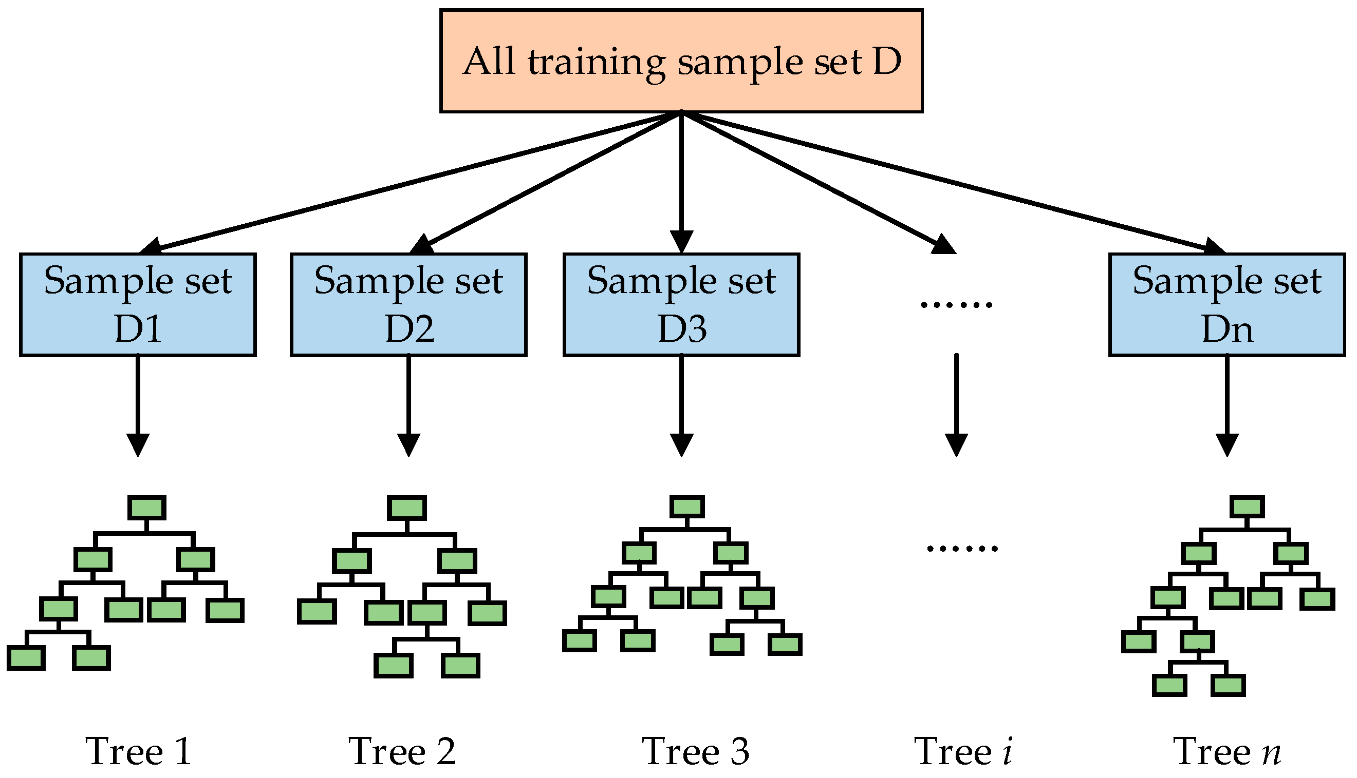
As the modeling of tunneling loads is a multi-parameter engineering problem, constructing π quantities based on dimensional analysis can achieve some dimension reduction effect, but the efficiency of the symbolic regression solution still needs to be improved. Therefore, it is necessary to eliminate unnecessary input parameters before model training. This paper presents a feature selection algorithm based on the random forest nonlinear model. The random forest method is an integrated algorithm based on decision trees [24] and can be used to evaluate the importance of each parameter for feature selection. The basic idea is illustrated in Figure 2. First, n samples are randomly extracted from the original dataset to generate n training sets. Based on these training sets, n decision tree models are then obtained. In each decision tree model, the parameters and samples are divided according to the Gini coefficient, so that each tree is constantly divided into different branches. Eventually, all the trees come together to form a random forest. When selecting the feature parameters based on the random forest model, the Gini coefficients are the calculation indices that determine the importance of each feature. In the regression decision tree, the Gini coefficient (GINI) of each node is actually the sample variance, as shown in Equation (1). Finally, the Gini index of each feature quantity in n trees is summarized and calculated to obtain the variable importance measure (VIM), so as to realize feature selection. Therefore, the feature selection method based on the random forest model has good applicability to nonlinear regression models.
GINI = 1 n i = 1 n ( y i y ¯ ) 2
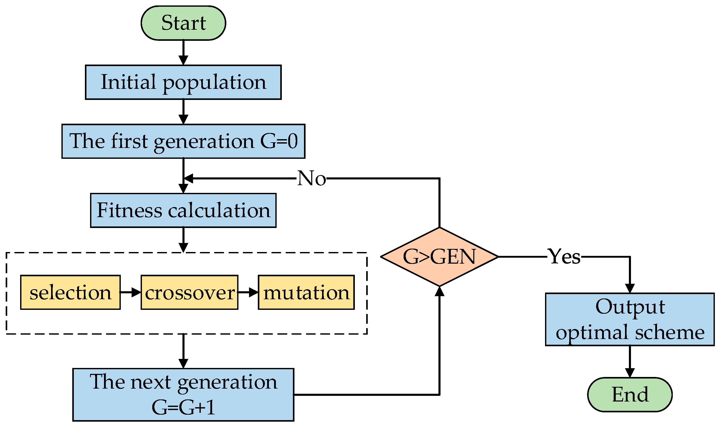
To output explicit load models that can describe the physical relationship between the parameters, a training model based on symbolic regression is proposed. After feature selection, the symbolic regression algorithm is applied to train the models. This is a nonlinear regression algorithm that automatically discovers rules and knowledge based on the data, without any prior assumptions about the functional form of the training model. Some fitness value (usually the mean absolute error) is taken as the optimization goal, and the optimal solution is discovered using a genetic algorithm [29]. Genetic algorithms are intelligent optimization algorithms that search for the optimal solution by simulating the natural evolution process [30]. Their basic operation process is shown in Figure 3. First, the population is initialized. The initialization settings include the number of individuals M, the number of superior individuals in each generation, and the maximum number of evolution generations GEN. At this time, the system will randomly generate M initial individuals, and then apply selection, crossover, and mutation operations based on the fitness of different individuals, to form the next-generation population. Successive generations continue to circulate and evolve until the maximum number of evolution generations is reached. Finally, the individual with the maximum fitness value is output as the optimal solution [31]. Compared with traditional optimization algorithms, which begin the iteration process from a single solution, the genetic algorithm starts searching from a series of randomly generated solutions, which increases the coverage of the search and reduces the risk of becoming trapped around a local optimal solution [31,32,33]. However, a single application of the genetic algorithm cannot fully represent the constraints of the optimization problem. In the symbolic regression algorithm, these constraints are reflected in the operation symbol and the complexity of the function solution, which are set by two parameters: “function” (operation symbol) and “parsimony_coefficient” (model simplicity coefficient). Both of these settings directly affect the model morphology. The tuning of the parameters will be discussed in detail in Section 4.3. In the process of modeling, several regression symbols that accord with the theoretical relationship are tested by the enumeration method, and then the symbol setting of the final modeling and load models are determined according to the “simple and effective” principle, known as “Ockham’s razor” [34]. The basic idea of this principle is: “Do not add an entity if it is not necessary.” A large number of mathematical and scientific studies have confirmed that when two models have the same effect, choosing the simpler one is more conducive to grasping the fundamental law and reflecting the essential characteristics [35,36,37].

3. Constructing π Quantities Based on Dimensional Analysis

Dimensions reflect the most essential attributes of physical parameters. Any physical parameter can be traced back to its definition or derivation source through dimensions. The parameters of tunneling loads typically fall into three categories: geological, operational, and those based on the equipment structure. According to the relevant investigation and mechanical analysis of the geological failure mechanism, and the statistical analysis of some geological parameters, it is found that geological parameters have some linear correlation, and the influence of some geological parameters on the tunneling loads can be considered in some basic mechanical parameters. For example, the influence of rock joints on the tunneling load can be reflected by the shear modulus of rock during exploration. Therefore, six basic mechanical parameters are determined for analysis. The specific parameters and their dimensions are presented in Table 1.
The П theorem is an important theorem about dimensional analysis, which states that every physical problem can be represented by several dimensionless powers of quantities [38], denoted by π. Based on the basic idea of the П theorem, the relationship between the tunneling loads and the parameters is as follows:
π F , T = g ( π 1 , π 2 , , π k )
Here, k = ( n 3 ) , n is the number of influencing parameters, and π 1 , π 2 , , π k , π F , T are the dimensionless π quantities composed of influencing parameters.
To construct the dimensionless π quantities mentioned in Equation (1), analysis and calculations are carried out through two steps: the selection of the basic quantities and the construction of π quantities.

3.1. Selection of the Basic Quantities

Basic quantities should be the core parameters reflecting the physical relationship. The selection of basic quantities directly determines the functional form of each π quantity. However, their selection method has some degree of freedom. Therefore, the basic quantities need to be determined by combining the characteristics of the specific problem. The basic quantity selection process in this paper is shown in Figure 4.
As the number of basic quantities should be equal to the number of basic dimensions of the research problem, and as there are three basic dimensions in a mechanical system (mass dimension M, length dimension L, and time dimension T), all the influencing parameters are divided into three groups according to their basic dimensions, as listed in Table 2. One parameter is then selected from each group as the basic quantity. Finally, based on the selected basic quantities, a dimensionless operation is performed on the remaining parameters to construct the π quantities. For the selection of the basic quantities in each dimensional group, this paper mainly considers three aspects: (i) whether it is the core parameter that has a key influence on the target quantity; (ii) whether it is a constant parameter that has a key influence on the target quantity, because it is difficult to identify the influence of constant parameters when exploring the physical laws among the parameters through data analysis, and this could easily result in analysis blind spots; and (iii) whether the dimensionality of a parameter is “concise,” because the construction of a π quantity essentially uses the basic quantity as a unit system to measure each parameter [12], which is a switch of measurement methods. It is found that choosing basic quantities with relatively simple dimensions is beneficial for obtaining more characteristic information. Considering the above principles, for the basic dimension M, the shear modulus G is selected as the basic quantity, as it is the core influencing parameter of the machine tunneling. For the basic dimension L, the cutter head diameter D is selected as the basic quantity. D is a constant parameter that has a direct influence on the total driving load and its dimension is very concise. For the basic dimension T, the cutter head speed ω is selected as the basic quantity, as it has a relatively simple dimension.

3.2. Constructing π Quantities

Based on the selected fundamental quantities, the π quantities are constructed through matrix operations. The independent variables x i and the target quantity y are expressed by the basic dimensions M, L, and T in the form shown in Equation (2), where α i , β i , γ i are the basic dimensional indices of the parameter x i , and α , β , γ are the basic dimensional indices of the target quantity y.
dim ( x i ) = M α i L β i T γ i , dim ( y ) = M α L β T γ
The selected basic quantities are denoted as x r , x s , x t , and the exponents to be solved are s i r , s i s , s i t , respectively. The following operations are performed for each parameter:
[ α r α s α t β r β s β t γ r γ s γ t ] [ s i r s i s s i t ] = [ α i β i γ i ] π i = x i x r s i r x s s i s x t s i t , π y = y x r s n r x s s n s x t s n t
The π quantities corresponding to the parameters v , μ , c , ρ , σ c , σ t , F , T are as follows:
π 1 = v D ω , π 2 = μ , π 3 = c G , π 4 = ρ ω 2 D 2 G , π 5 = σ c G , π 6 = σ t G , π F = F G D 2 , π T = T G D 3

4. Case Study

After obtaining the π quantities through dimensional analysis, they are trained on engineering data. In this paper, the calculations are based on in situ tunneling data from a construction section of the Yin-Song Project in Jilin Province, China, which is being constructed using a TBM with a diameter of 8.03 m. The length of the researched construction section is about 600 m. According to the geological exploration report, the stratum which the tunnel passes through is mainly composed of granite, which is a massive structure, and the mineral composition is mainly feldspar and quartz. The surrounding rocks are classified as granite II and III (according to China’s “engineering rock mass classification standards”). The statistical characteristics of each parameter in the tunneling data are shown in Table 3.
The calculation mainly includes three parts: data preprocessing, feature selection of the parameters, and model training.

4.1. Preprocessing of In Situ Tunneling Data

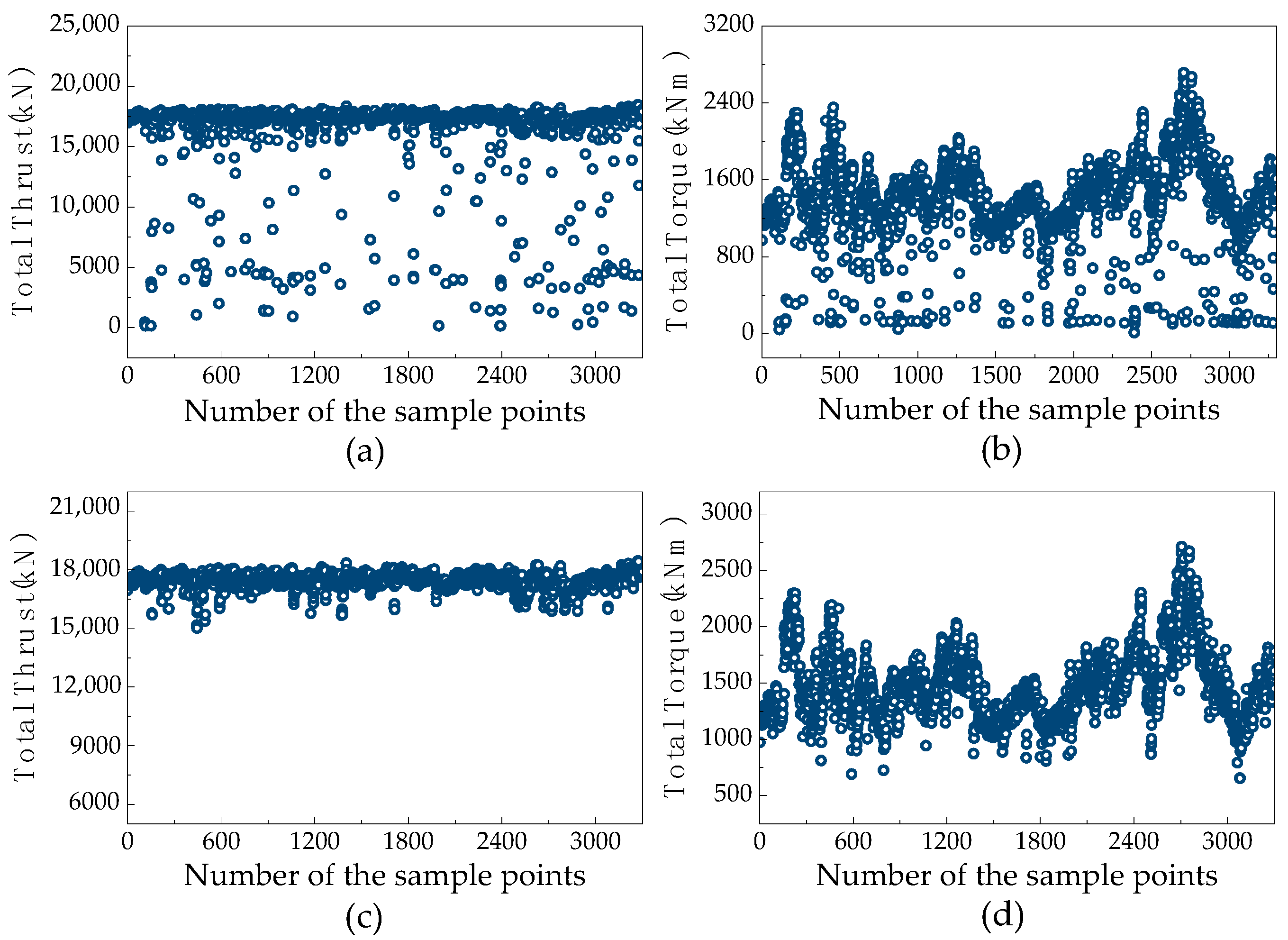
There are some outliers in the original tunneling data files of the Yin-Song Project, as shown in Figure 5a,b. These outliers mainly include null push data and abnormal data. When any of the operating parameters, such as the tunneling speed, cutter head speed, total thrust, and total torque, is 0 or close to 0, they are assumed to be “null push” data [28,39]. Such data are eliminated directly through numerical screening. Outliers usually exhibit the characteristics of mutation relative to their surrounding data points. However, although some of these abrupt data are outliers, others may be caused by geological changes. Therefore, it is necessary to combine professional knowledge with statistical methods to eliminate abnormal data effectively and maximize the retention of the regular characteristics of data. Load mutations caused by geological changes often affect more than one data point, so the difference method combined with box diagrams is proposed to distinguish the abnormal data. First, the forward and backward differences of all total thrust and torque data are calculated, and then the outliers in the difference results are identified by the box diagram method. Finally, the intersection of the forward and backward difference outliers is noted, and the corresponding load data points are identified as abnormal values. The union of the total thrust and torque abnormal values constitutes the abnormal data of the project. Compared with a direct statistical method for identifying the outliers of the tunneling load, this approach has the advantage that it, not only deals with anomalies effectively, but also avoids the mistake of deleting maximum or minimum values that deviate from the overall data mean, but exhibit regular changes. The box diagram method is a statistical technique for outlier detection when processing data. Unlike the 3σ rule, Z-score method, and so on, it does not presuppose the data distribution and follows the original characteristics of the data [40]. Its structure and outlier identification method are shown in Figure 6. A total of five statistics are calculated based on the data to be identified: median, lower quartile (Q1), upper quartile (Q3), lower limit (Q1 − 1.5IQR), and upper limit (Q3 + 1.5IQR), where IQR is the difference between the upper quartile and the lower quartile. Data sample points with values less than the lower limit or greater than the upper limit are considered to be outliers. The load data from the Yin-Song Project after outlier processing are shown in Figure 5c,d.
Considering the large differences in the magnitude of each π quantity, the dataset should be normalized before the machine learning algorithm is used to train the model. This prevents the magnitude from affecting the weight of different features. In this paper, decimal scaling normalization is used to restrict the data to the range 0–10. The calculation method is as follows:
x i = x i 10 j
where j is the smallest integer that makes max ( x i ) < 10 .

4.2. Feature Selection of Input Parameters

In the process of feature selection, to reduce the risk of becoming trapped around local optimal solutions, the union of 10 calculation results is selected as the final feature parameter. The dimensionless input parameters π 1 , π 2 , π 3 , π 4 , π 5 , π 6 calculated in Section 3.2 are trained with π F and π T as target quantities, respectively. When π T is used as the target quantity for feature selection, there is a very high correlation between π 1 and the target quantity, which leads to other more important feature parameters being neglected in the automatic calculation process; that is, a local optimal solution appears. Therefore, π 2 , π 3 , π 4 , π 5 , π 6 are further used as the input parameters for feature screening, and the union of two calculations is taken as the final result. The calculation results are as follows:
{ π F = f ( π 2 , π 3 , π 4 , π 5 , π 6 ) π T = g ( π 1 , π 2 , π 3 , π 5 , π 6 )

4.3. Modeling Based on Symbolic Regression Algorithm

In this study, the initial population number is set to 1000, the evolutionary algebra is set to 20, and the dominant number of each generation is set to 20. The data we are using have been normalized, so the range of constants is set as 0–10. The constraints on the complexity of the training model and the operation symbols are critical. When the model complexity is too high or there are too many operation symbols, the model will be very complex and cumbersome, whereas when the model setting is too simple, the risk of invalid solutions increases. In this algorithm, the rationality of the model is controlled by setting the parsimony_coefficient and function. Trial calculations show that, for training the tunneling load models in this paper, setting the parsimony_coefficient to be less than the default value of 0.001 increases the model complexity, but does not change R2 significantly. Therefore, the parsimony_coefficient is set to 0.001 in the modeling process. As for the setting of function, considering the theoretical relationship between the parameters and the target quantity, the five symbol setting schemes shown in Figure 7 are used to train the model. Five random sampling calculations are then carried out for each scheme and the R2 values are recorded. Through comparative analysis, reasonable model symbols are then determined according to the principle of Ockham’s razor.
Figure 8 shows how R2 changes under different regression symbol settings. In the thrust modeling, when the regression symbol is “add, mul”, R2 is higher than for other symbols and the fluctuation range is small, that is, the model recognition is relatively stable. Therefore, the regression symbol for thrust modeling is set to “add, mul”. For torque modeling, the regression symbol “add, mul” gives a significantly higher R2 value than “add” and “add, mul, div, sqrt, log”, but a similar value to “add, mul, div” and “add, mul, div, sqrt”. However, the model complexity of the latter two symbols is significantly higher, and the model becomes unstable. Therefore, following the principle of Ockham’s razor, it is more reasonable to use the “add, mul” regression symbol for torque modeling.
Based on the above settings, the tunneling data from the Yin-Song Project are randomly divided into a training set and a test set at a ratio of 7:3. The total thrust and total torque are modeled based on the training dataset, and the calculated results are given by Equation (8). The R2 of the thrust and torque models in the independent test dataset are 0.95 and 0.81, respectively. The measured and predicted values in the test set are compared in Figure 9. The serial number of the sample points in the figure is the number of sample points according to the construction sequence.
{ F G D 2 = ( c + σ t + σ c 10 2 ) c G 2 10 2 T G D 3 = ( v D ω + σ c G 10 6 ) σ t G
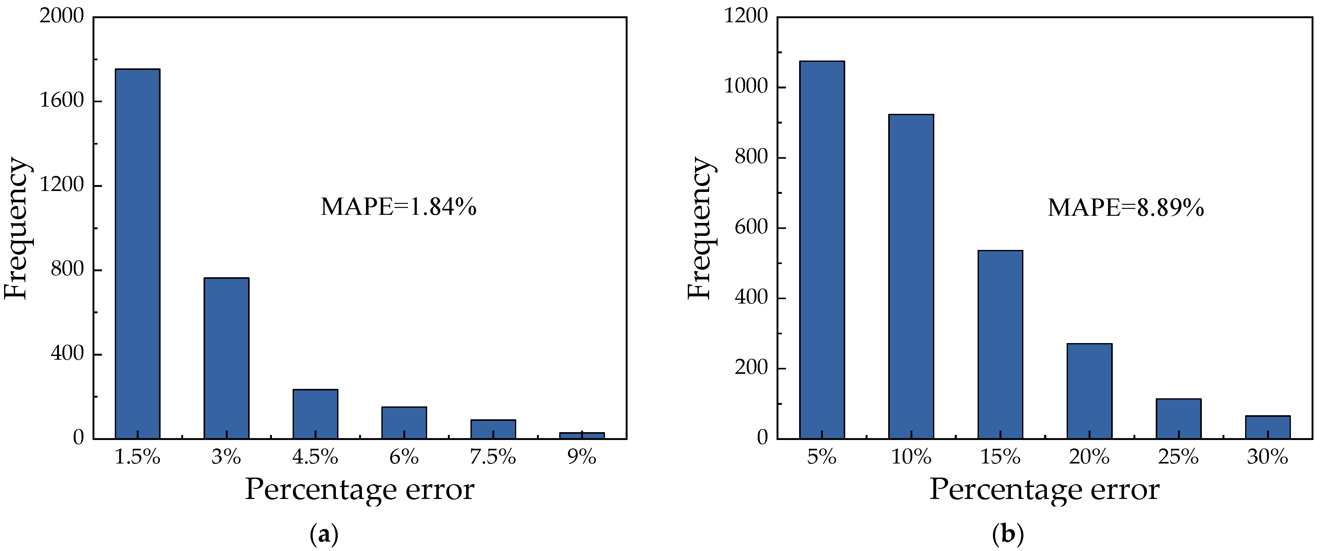
After dimension reduction, the load models are as shown in Equation (9). The statistical results of the prediction error of the model in the total dataset are shown in Figure 10. The thrust prediction error is less than 6% for 95% of the data, and the torque prediction error is less than 20% for 92% of the data. This indicates that the prediction model for tunneling total loads accurately reflects the tunneling total load values in actual engineering projects.
{ F = ( c + σ t + σ c 10 - 2 ) c D 2 G 10 - 2 T = ( v ω D G + σ c 10 6 ) σ t D 3 G

4.4. Discussion

Analyze the load model Formula (9) and convert it into the form shown in Formula (10). It is found that the thrust and torque models have quadratic and cubic power function relations, with the diameter of the cutter head D, respectively, which conforms to the basic theory of mechanical equilibrium. In addition, the parametric relations given by the models indicate that the ratios of cohesion c, compressive strength σc, and tensile strength σt to shear modulus G are the important factors affecting the total loads under similar hard rock geological conditions. The rock cohesion c and compressive strength σt have key influences on the total thrust and the total torque, respectively. In the torque model, v/ω is actually the penetration degree of the cutter head. Therefore, the penetration degree of the cutter head is also an important factor affecting the total tunneling torque.
{ F = ( c G + σ t G + σ c G 10 - 2 ) 10 - 2 c D 2 T = σ t ( v ω D 2 + 10 6 σ c G D 3 )
To further evaluate the tunneling load prediction model, general linear regression and artificial neural network algorithms are used to model and predict the tunneling total loads based on the same engineering data samples. The input parameters are the same as for the symbolic regression. The R2 and MAPE (mean absolute percentage error) of five random samples in the independent test set are selected and averaged. The results are presented in Table 4, and the linear regression model is described by Equations (11) and (12). Analysis shows that the prediction effect of the linear regression model is slightly better than that of the other two algorithms. However, according to Equations (11) and (12), the relationship between certain parameters in the model and the target quantity is obviously inconsistent with the theoretical laws. For example, in Equation (11) there is a negative correlation between the compressive strength σ c of the rock and the total thrust F, and in Equation (12) there is a negative correlation between the cutter head speed ω and the total torque T. There is no significant difference in the prediction effect between the symbolic regression model and the neural network model. However, as can be seen from Equation (10) and its analysis, the advantage of the symbolic regression model is that it provides an explicit physical relationship model, which not only conforms to the basic theoretical relationship, but also satisfies the physical rules of dimensional uniformity. In conclusion, based on the modeling method proposed in this paper, load models with both prediction accuracy and interpretability can be obtained through the training of engineering data.
F G D 2 = 2.67 10 - 2 v D ω 23.9 μ + 9.56 c G + 27.4 ρ ω 2 D 2 G 0.193 σ c G + 1.77 σ t G + 4.33 F = 2.67 10 - 2 v ω G D 23.9 μ G D 2 + 9.56 c D 2 + 27.4 ρ ω 2 D 4 0.193 σ c D 2 + 1.77 σ t D 2 + 4.33 G D 2
T G D 3 = 1.28 v D ω + 0.257 μ 0.152 c G 0.102 ρ ω 2 D 2 G + 3.67 10 4 σ c G + 2.53 10 2 σ t G 4.85 10 2 T = 1.28 v ω G D 2 + 0.257 μ G D 3 0.152 c D 3 0.102 ρ ω 2 D 5 + 3.67 10 4 σ c D 3 + 2.53 10 2 σ t D 3 4.85 10 2 G D 3

5. Conclusions

Aiming at the problem of modeling tunneling loads, a modeling method based on symbolic regression has been proposed in this paper. In this method, dimensionless processing is carried out on the original parameters through dimensional analysis, allowing the nonlinear combination relationship between the parameters to be constructed and the dimensionless parameters (π quantities) to be obtained in accordance with some potential physical connotations. Taking the π quantities as the input parameters for the subsequent calculations and model training is equivalent to providing physical constraints on the training process, and ensures that the modeling process satisfies the relevant dimensional rules, which helps the symbolic regression training to obtain a more efficient and reasonable load model. In addition, the dimensionless processing of the parameters also achieves the effect of dimensionality reduction, reducing the initial nine parameters to six. To further improve the efficiency of the symbolic regression modeling, feature selection is applied before model training to eliminate unnecessary input parameters. To avoid the constraint of a priori assumptions on the function relationship between π quantities, feature selection is based on a random forest model. Finally, the principle of Ockham’s razor is applied to complete the symbolic regression modeling. The results show that the method can obtain explicable load models based on the potential physical relationship between the parameters, while guaranteeing the accuracy of the predictions. The model also satisfies the basic mechanical theoretical relations and physical dimensional rules, and the form is simple. This improves the practicability of machine learning modeling, and provides a reference for construction excavation. The modeling method described in this paper provides a new concept for obtaining training models that are interpretable and conform to the relevant physical rules.
It is important to emphasize that the modeling method combining dimensional analysis, feature selection, and symbolic regression algorithm in this paper can be applied to other projects. Moreover, the models in Equation (9) based on the engineering case of Jilin Project can provide a reference for similar working conditions if needed.

Author Contributions

Conceptualization, Q.Z.; methodology, Q.Z.; funding acquisition, Q.Z.; supervision, Q.Z.; validation, L.Z., S.Z. and S.L.; formal analysis, L.Z.; writing—original draft, L.Z.; writing—review and editing, Q.Z. and L.Z. All authors have read and agreed to the published version of the manuscript.

Funding

This research was supported by National Key R&D Program of China [No. 2018YFB1702505], National Natural Science Foundation of China [No. 11872269], and Natural Science Foundation of Tianjin [No. 18JCYBJC19600].

Institutional Review Board Statement

Not applicable.

Informed Consent Statement

Not applicable.

Data Availability Statement

The raw/processed data required to reproduce these findings cannot be shared at this time as the data also forms part of an ongoing study.

Conflicts of Interest

The authors declare that they have no conflict of interest to report regarding the present study.

References

  1. Stachowiak, G.P.; Stachowiak, G.W.; Podsiadlo, P. Automated classification of wear particles based on their surface texture and shape features. Tribol. Int. 2008, 41, 34–43. [Google Scholar] [CrossRef]
  2. Hassanpour, J.; Ghaedi Vanani, A.A.; Rostami, J.; Cheshomi, A. Evaluation of common TBM performance prediction models based on field data from the second lot of Zagros water conveyance tunnel (ZWCT2). Tunn. Undergr. Space Technol. 2016, 52, 147–156. [Google Scholar] [CrossRef]
  3. Salimi, A.; Rostami, J.; Moormann, C.; Delisio, A. Application of non-linear regression analysis and artificial intelligence algorithms for performance prediction of hard rock TBMs. Tunn. Undergr. Space Technol. 2016, 58, 236–246. [Google Scholar] [CrossRef]
  4. Armaghani, D.J.; Koopialipoor, M.; Marto, A.; Yagiz, S. Application of several optimization techniques for estimating TBM advance rate in granitic rocks. J. Rock Mech. Geotech. Eng. 2019, 11, 779–789. [Google Scholar] [CrossRef]
  5. Koopialipoor, M.; Tootoonchi, H.; Jahed Armaghani, D.; Tonnizam Mohamad, E.; Hedayat, A. Application of deep neural networks in predicting the penetration rate of tunnel boring machines. Bull. Eng. Geol. Environ. 2019, 78, 6347–6360. [Google Scholar] [CrossRef]
  6. Dalong, J.; Zhichao, S.; Dajun, Y. Effect of Spatial Variability on Disc Cutters Failure During TBM Tunneling in Hard Rock. Rock Mech. Rock Eng. 2020, 53, 4609–4621. [Google Scholar] [CrossRef]
  7. Rispoli, A.; Ferrero, A.M.; Cardu, M. From Exploratory Tunnel to Base Tunnel: Hard Rock TBM Performance Prediction by Means of a Stochastic Approach. Rock Mech. Rock Eng. 2020, 53, 5473–5487. [Google Scholar] [CrossRef]
  8. Wei, M.; Song, Y.; Wang, X.; Peng, J. Safety diagnosis of TBM for tunnel excavation and its effect on engineering. Neural Comput. Appl. 2021, 33, 997–1005. [Google Scholar] [CrossRef]
  9. Ates, U.; Bilgin, N.; Copur, H. Estimating torque, thrust and other design parameters of different type TBMs with some criticism to TBMs used in Turkish tunneling projects. Tunn. Undergr. Space Technol. 2014, 40, 46–63. [Google Scholar] [CrossRef]
  10. Zhou, X.P.; Zhai, S.F. Estimation of the cutterhead torque for earth pressure balance TBM under mixed-face conditions. Tunn. Undergr. Space Technol. 2018, 74, 217–229. [Google Scholar] [CrossRef]
  11. Zhang, Q.; Su, C.; Qin, Q.; Cai, Z.; Hou, Z.; Kang, Y. Modeling and prediction for the thrust on EPB TBMs under different geological conditions by considering mechanical decoupling. Sci. China Technol. Sci. 2016, 59, 1428–1434. [Google Scholar] [CrossRef]
  12. Rostami, J.; Ozdemir, L. A new model for performance prediction of hard rock TBMs. Rect Proc. 1993, 50, 793–809. [Google Scholar]
  13. Rostami, J.; Ozdemir, L.; Nilson, B. Comparison between CSM and NTH hard rock TBM performance prediction models. In Proceedings of the Annual Technical Meeting of the Institute of Shaft Drilling Technology, Las Vegas, NV, USA, 1–3 May 1996; pp. 1–10. Available online: https://www.researchgate.net/publication/237801456 (accessed on 15 June 2021).
  14. Liu, H.P. Study on TBM Cutterhead Working Principle. Appl. Mech. Mater. 2012, 152–154, 1612–1618. [Google Scholar] [CrossRef]
  15. Young, K.T.; Jin, Y.H.; Jin, S.Y. A comparative study on the TBM disc cutter wear prediction model. J. Korean Tunn. Undergr. Space Assoc. 2014, 16. [Google Scholar] [CrossRef] [Green Version]
  16. Shi, H.; Yang, H.; Gong, G.; Wang, L. Determination of the cutterhead torque for EPB shield tunneling machine. Autom. Constr. 2011, 20, 1087–1095. [Google Scholar] [CrossRef]
  17. Wang, L.; Gong, G.; Shi, H.; Yang, H. Modeling and analysis of thrust force for EPB shield tunneling machine. Autom. Constr. 2012, 27, 138–146. [Google Scholar] [CrossRef]
  18. Zhang, Q.; Huang, T.; Huang, G.Y.; Cai, Z.X.; Kang, Y.L. Theoretical model for loads prediction on shield tunneling machine with consideration of soil-rock interbedded ground. Sci. China Technol. Sci. 2013, 56, 2259–2267. [Google Scholar] [CrossRef]
  19. Zhang, Q.; Qu, C.Y.; Cai, Z.X.; Kang, Y.L.; Huang, T. Modeling of the thrust and torque acting on shield machines during tunneling. Autom. Constr. 2014, 40, 60–67. [Google Scholar] [CrossRef]
  20. Zhang, H.M.; Wu, X.G.; Zeng, W.H. Experimental study on earth pressure balance shield tunneling and mathematical model. Chin. J. Rock Mech. Eng. 2005, S2, 5762–5766. (In Chinese) [Google Scholar]
  21. Entacher, M.; Lorenz, S.; Galler, R. Tunnel boring machine performance prediction with scaled rock cutting tests. Int. J. Rock Mech. Min. 2014, 70, 450–459. [Google Scholar] [CrossRef]
  22. Zhang, Z.Q.; Li, T.; Han, A.M. Prediction Model of Shield Driving Rate and Cutterhead Torque and Its Formation Adaptability in Complex Strata. Tunn. Constr. 2016, 36, 1449–1455. (In Chinese) [Google Scholar]
  23. Yagiz, S. New equations for predicting the field penetration index of tunnel boring machines in fractured rock mass. Arab. J. Geosci. 2017, 10, 33. [Google Scholar] [CrossRef]
  24. Li, J.; Li, P.; Guo, D.; Li, X.; Chen, Z. Advanced prediction of tunnel boring machine performance based on big data. Geosci. Front. 2021, 12, 331–338. [Google Scholar] [CrossRef]
  25. Sun, W.; Shi, M.; Zhang, C.; Zhao, J.; Song, X. Dynamic load prediction of tunnel boring machine (TBM) based on heterogeneous in-situ data. Autom. Constr. 2018, 92, 23–34. [Google Scholar] [CrossRef]
  26. Zheng, Z.; Chen, K.; Zhang, Q. Identification of Loads on Shield Tunneling Machines Based on PSO-SVM Method. Appl. Mech. Mater. 2013, 392, 746–749. [Google Scholar] [CrossRef]
  27. Yagiz, S.; Karahan, H. Prediction of hard rock TBM penetration rate using particle swarm optimization. Int. J. Rock Mech. Min. 2011, 48, 427–433. [Google Scholar] [CrossRef]
  28. Zhang, Q.L.; Liu, Z.; Tan, J. Prediction of geological conditions for a tunnel boring machine using big operational data. Autom. Constr. 2019, 100, 73–83. [Google Scholar] [CrossRef]
  29. Köktürk-Güzel, B.E.; Beyhan, S. Symbolic Regression Based Extreme Learning Machine Models for System Identification. Neural Process. Lett. 2021, 53, 1565–1578. [Google Scholar] [CrossRef]
  30. Nijhout, F. An introduction to genetic algorithms. Complexity 1997, 2, 39–40. [Google Scholar] [CrossRef]
  31. Zheng, Q.; Sha, J.; Fang, C. An effective genetic algorithm to VDA with discontinuous “on-off” switches. Sci. China Earth Sci. 2012, 55, 1345–1357. [Google Scholar] [CrossRef]
  32. Xing, X.; Liu, Y.; Garg, A.; Ma, X.; Yang, T.; Zhao, L. An improved genetic algorithm for determining modified water-retention model for biochar-amended soil. Catena 2021, 200, 105143. [Google Scholar] [CrossRef]
  33. Mahardhika, T. Hybrid Algorithm as alternative method for optimization, a combination Genetic Algorithm and Particle Swarm Optimization. J. Phys. Conf. Ser. 2021, 1764, 12040. [Google Scholar] [CrossRef]
  34. Rodriguez-Fernández, J. Ockham’s razor. Endeavour 1999, 23, 121–125. [Google Scholar] [CrossRef]
  35. Sonnergaard, J.M. Ockham’s Razor Applied on Pharmaceutical Powder Compaction Models. J. Pharm. Sci. 2021, 110, 989–996. [Google Scholar] [CrossRef]
  36. Stanhill, G. Total, global and surface solar radiation: The case for Ockham’s razor. Weather 2018, 73, 117. [Google Scholar] [CrossRef]
  37. Mirko, F.; Mazen, A. The Ockham’s razor applied to COVID-19 model fitting French data. Annu. Rev. Control 2021. prepublish. [Google Scholar]
  38. Buckingham, E. On physically similar systems. J. Wash. Acad. Sci. Wash. DC 1914, 4, 345–376. [Google Scholar]
  39. Hou, S.K.; Liu, Y.R.; Li, C.Y.; Qin, P.X. Dynamic Prediction of Rock Mass Classification in the Tunnel Construction Process based on Random Forest Algorithm and TBM in situ Operation Parameters. Iop Conf. Ser. Earth Environ. Sci. 2020, 570, 052056. [Google Scholar] [CrossRef]
  40. Li, A.; Feng, M.; Li, Y.; Liu, Z. Application of Outlier Mining in Insider Identification Based on Boxplot Method. Procedia Comput. Sci. 2016, 91, 245–251. [Google Scholar] [CrossRef] [Green Version]
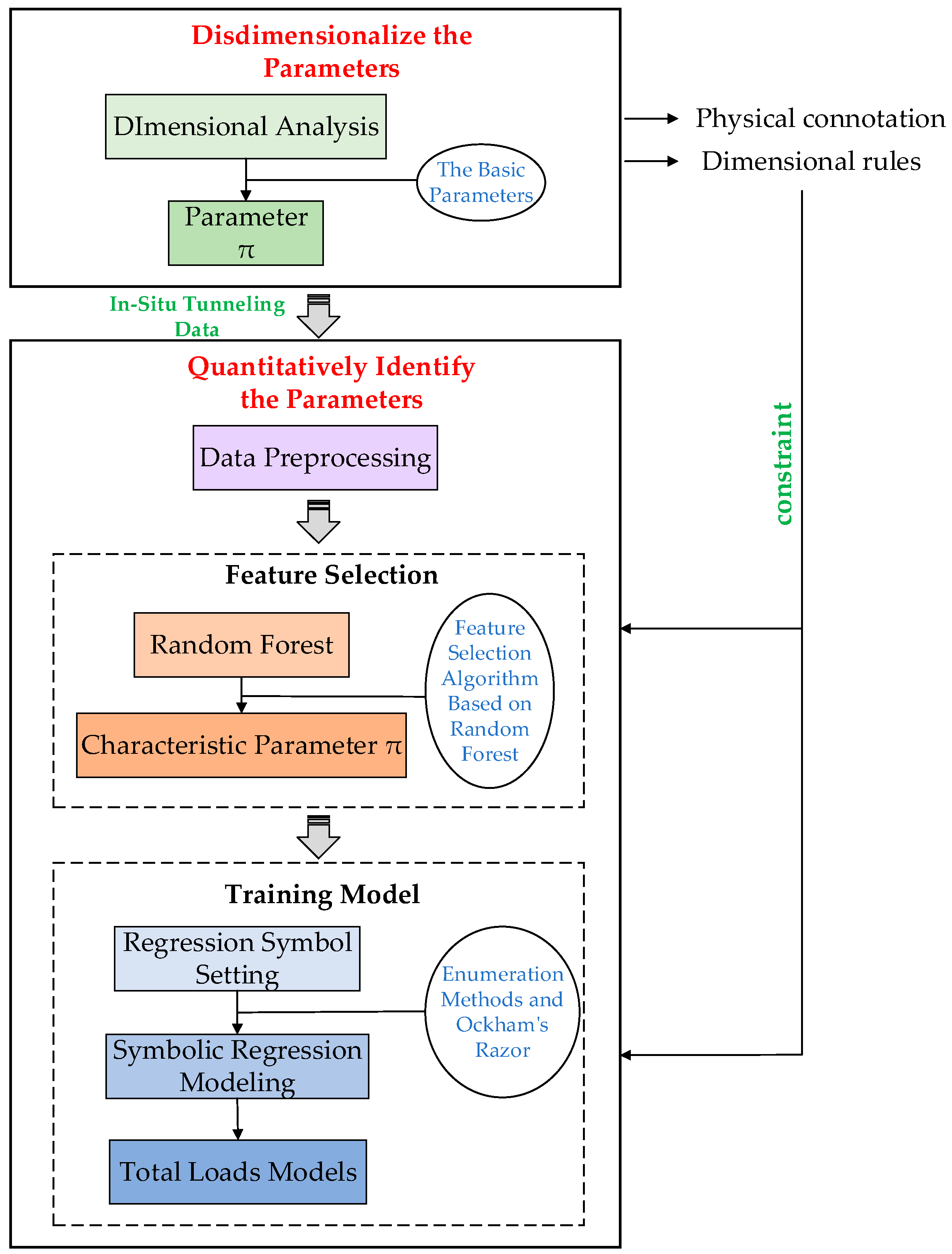
Figure 1. Modeling process.
Applsci 11 05671 g001
Figure 2. Basic concept of the random forest algorithm.
Applsci 11 05671 g002
Figure 3. Basic operation process of genetic algorithm.
Applsci 11 05671 g003
Figure 4. The basic quantity selection process.
Applsci 11 05671 g004
Figure 5. Data of tunneling loads in the Yin-Song Project: (a) total thrust before outlier processing, (b) total torque before outlier processing, (c) total thrust after outlier processing, (d) total torque after outlier processing.
Applsci 11 05671 g005
Figure 6. Box diagram structure.
Applsci 11 05671 g006
Figure 7. Regression symbol setting schemes.
Applsci 11 05671 g007
Figure 8. R2 with different regression symbol settings: (a) the total thrust, (b) the total torque.
Applsci 11 05671 g008
Figure 9. Comparison between the predicted values and the measured values of the dimensionless load models: (a) the total thrust, (b) the total torque.
Applsci 11 05671 g009
Figure 10. Statistical results of prediction error on the total set: (a) the total thrust, (b) the total torque.
Applsci 11 05671 g010
Table 1. Parameters and their dimensions.
Physical ParametersDimension
Machine ParametersCutterhead diameter D   ( m ) L
Operating ParametersDriving speed v   ( m / s ) L T−1
Cutterhead rotation speed ω   ( r / min ) T−1
Geologic ParametersRock density ρ   ( g / cm 3 ) M L−3
Shear modulus G   ( MPa ) M L−1 T−2
Poisson’s ratio μ
Cohesive force c   ( kPa ) M L−1 T−2
Compressive strength σ c   ( MPa ) M L−1 T−2
Tensile strength σ t   ( MPa ) M L−1 T−2
Target ParametersTotal thrust F   ( kN ) M L T−2
Total torque T   ( kN m ) M L2 T−2
Table 2. Grouping of the influencing parameters based on basic dimensions.
Basic Dimensions MBasic Dimensions LBasic Dimensions T
Physical ParametersDimensionPhysical ParametersDimensionPhysical ParametersDimension
ρ M L−3 D L v L T−1
G M L−1 T−2 v L T−1 G M L−1 T−2
c M L−1 T−2 ρ M L−3 c M L−1 T−2
σ c M L−1 T−2 G M L−1 T−2 σ c M L−1 T−2
σ t M L−1 T−2 c M L−1 T−2 σ t M L−1 T−2
σ c M L−1 T−2
σ t M L−1 T−2
ω T−1
Table 3. The statistical characteristics of the parameters.
Physical ParametersMaximumMinimumAverage
Operating ParametersDriving speed v   ( mm / min ) 81.001.0018.04
Cutterhead rotation speed ω   ( r / min ) 7.000.245.75
Geologic ParametersRock density ρ   ( g / cm 3 ) 2.702.642.65
Shear modulus G   ( MPa ) 7.153.754.04
Poisson’s ratio μ 0.270.230.26
Cohesive force c   ( kPa ) 1.911.451.50
Compressive strength σ c   ( MPa ) 106.5774.9978.82
Tensile strength σ t   ( MPa ) 6.594.754.96
Target ParametersTotal thrust F   ( kN ) 18,458.00151.0016,843.48
Total torque T   ( kN m ) 2712.0012.001408.90
Table 4. Comparison of tunneling total load models under different modeling methods.
Total ThrustTotal Torque
R2MAPEModelTheoretical RelationshipR2MAPEModelTheoretical Relationship
SR0.951.82%Explicitreasonable0.818.83%explicitreasonable
LR0.961.55%Explicitunreasonable0.848.13%explicitunreasonable
ANN0.951.71%hidden layerunknown0.818.33%hidden layerunknown
Publisher’s Note: MDPI stays neutral with regard to jurisdictional claims in published maps and institutional affiliations.