Approximate Image-Space Multidirectional Occlusion Shading Model for Direct Volume Rendering

Abstract

Understanding and perceiving three-dimensional scientific visualizations, such as volume rendering, benefit from visual cues produced by the shading models. The conventional approaches are local shading models since they are computationally inexpensive and straightforward to implement. However, the local shading models do not always provide proper visual cues since non-local information is not sufficiently taken into account for the shading. Global illumination models achieve better visual cues, but they are often computationally expensive. It has been shown that alternative illumination models, such as ambient occlusion, multidirectional shading, and shadows, provide decent perceptual cues. Although these models improve upon local shading models, they still require expensive preprocessing, extra GPU memory, and a high computational cost, which cause a lack of interactivity during the transfer function manipulations and light position changes. In this paper, we proposed an approximate image-space multidirectional occlusion shading model for the volume rendering. Our model was computationally less expensive compared to the global illumination models and did not require preprocessing. Moreover, interactive transfer function manipulations and light position changes were achievable. Our model simulated a wide range of shading behaviors, such as ambient occlusion and soft and hard shadows, and can be effortlessly applied to existing rendering systems such as direct volume rendering. We showed that the suggested model enhanced the visual cues with modest computational costs.

1. Introduction

Direct volume rendering is a conventional technique to visualize volumetric datasets, such as measured medical data and scientific simulation data. The direct volume rendering is beneficial when the rendering provides proper visual cues to emphasize the spatial relationships within the data. The visual cues can be further enhanced by improving the shading models in the rendering pipeline. The realism supported by the improved shading models enables the user to understand the data better since the rendering images become realistic, similar to a natural image. Therefore, many approaches have been proposed to enhance the conventional shading models.

On the one hand, many simplified shading models from the global illumination models [1] have been developed for interactive rendering performance, such as ambient occlusion and shadow maps, which are volumetric approaches. These techniques interactively provide perceptually better visual cues in the rendering. However, most of the techniques require long computing times for preprocessing, a substantial amount of extra GPU memory, multiple additional rendering passes, or all of these. Moreover, the rendering performance becomes significantly degraded if the additional cost scales relative to the size of the input volume data. Some of the approximations [2,3] interactively operate on-the-fly and do not require additional GPU memory. However, they are limited to a particular rendering technique such as slice-based direct volume rendering, and the additional computation is proportional to the size of the volume data.

On the other hand, to overcome the performance degradation proportional to the data size, image-space occlusion techniques have been proposed for the polygonal rendering [4,5,6,7,8,9] that is widely used in computer graphics and the gaming industry. The color, normal, and depth of a scene are rendered to buffers, and the occlusion is computed with the depth and normal buffers. The benefits of these methods are that they are independent of the rendering engine and can be applied to any rendering pipeline by merely adding a screen-space pass. Furthermore, the computation is much less compared to the volumetric approaches.

In this work, we present an approximate image-space multidirectional occlusion shading (ISMOS) model for the direct volume rendering. Our model, ISMOS, simulates the global illumination effects in a simplified manner. ISMOS utilizes the rendered depth and normal buffers for the occlusion shading computation at the end of the direct volume-rendering pipeline. ISMOS does not require preprocessing, nor extra GPU memory for the entire volume data. Since the model is operated as an additional computation in the shader, ISMOS can be easily employed in any volume-rendering pipeline. Besides, the transfer function manipulations and light property changes, including light positions, can be interactively executed on-the-fly without interrupting the rendering since ISMOS utilizes the rendered buffer information on the GPU memory. ISMOS simulates various light sources, whereas previous models simulated only ambient and directional light sources. For the sampling strategy, while previous models sampled test points within a hemisphere centered at each pixel, ISMOS takes sample points along a ray between a pixel and the light source to calculate the amount of light transferred to the pixel. Note that preprocessing indicates the light volume generation before the ray casting volume rendering, and the light volume is repeatedly generated whenever the light parameters and transfer function parameters are changed in other approaches.

Figure 1a illustrates the ISMOS model setup, including the volume-rendered image-space, eye position, and light source. The volume-rendered image-space contains the color, depth, and normal information stored in the renderbuffers. The eye position indicates the camera location, and the light source is placed on a hemisphere with the radius R, centered at the center of the image-space. Figure 1b,c shows three different light sources, including point, area, and ambient lights. Note that the light source in (a) is an example of the area light source with the radius d. Since our image-space model does not require notable extra computation time, ISMOS easily enabled us to manipulate multiple light sources. The multiple directional light sources were difficult to apply in the previous image-space approaches because the hemispheres centered at the pixels were not directional. Besides, we applied an opacity threshold for the shading effect estimation on the opaque pixels to make the inner volume structures stand out, which allowed us to create renderings accommodating multiple transparent layers with different opacity values. We also handled transparent objects efficiently by applying a transmittance approximation with a smooth function, which can be easily performed in a volume-rendering pass, as presented in Figure 2. The approximated functional form of the transmittance describes the opacity values, which allowed us to represent all opacity values over the depth with only one parameter per pixel. Figure 3 presents the rendering pipeline. We extended the conventional volume rendering with frame buffers to simulate various occlusion shading models.

Our major contributions in this work include:

• An interactive approximate image-space multidirectional occlusion shading model applicable to the conventional direct volume-rendering pipeline without preprocessing and additional GPU memory;
• The simulation of light sources, including ambient occlusion and soft and hard shadows as a unified model;
• The handling of multiple directional lights with only a minor additional overhead;
• A multi-layered view for transparent scenes.

2. Related Work

Volume rendering has been widely used to explore volumetric datasets and provides useful insights into the volumetric datasets. For a better understanding of the data, illumination models have been intensively studied over the decades. Various optical approximation models, such as emission–absorption models [10], have been widely employed to build up the volume rendering system. Levoy [11] presented a local illumination model with gradients in the volume rendering, which enhanced the visual cues.

However, the locally illuminated volume rendering might not give sufficient depth cues that enable unobstructed visualization of complicated features in the volumetric data. Kniss et al. [12] proposed a simple and effective interactive shading model that captured volumetric light attenuation effects, including volumetric shadows. They utilized a direct and indirect light contribution to render a translucent material. Hernell et al. [13] achieved an interactive global light propagation in the direct volume rendering. Their technique was nearly physically correct, unlike the model by Kniss et al. [12]. Tarini et al. [14] presented ambient occlusion and edge cueing for molecular visualizations. Their approach interactively enhanced the visual cues for the understanding of complex molecular surface renderings.

Ambient occlusion has been applied in volume rendering to improve visual quality and understanding. Díaz et al. [15] used summed-area tables to compute the ambient occlusion and halos. They presented a vicinity occlusion map (VOM) and a density summed-area table (DSAT) to enhance depth perception for the volumetric data. However, the VOM works in limited circumstances, and the DSAT for the volume data requires extra 3D texture memory with a long preprocessing time. Local ambient occlusion in the volume rendering was proposed by Hernell et al. [16]. The approach is a gradient-free shading model and, therefore, less sensitive to noise. In their work, an extra 3D texture was generated to hold the emissive color and the ambient light of each voxel. However, the extra 3D texture was regenerated whenever the transfer function was changed. Recently, advanced illumination models [17,18,19,20,21,22,23,24] for the volume rendering have been introduced. Ropinski et al. [23] presented an interactive volume rendering with ambient occlusion and color bleeding. Lindemann and Ropinski [19] showed advanced light material interactions. Moving light sources [21,22] have also been applied in the interactive volume rendering. In the work of [21,22], the volumetric lighting was simulated for the scattering and shadowing. However, all of these studies utilized extra 3D texture memory to store the new volumetric lighting information, which required additional preprocessing operations. Since the rendering only needed to fetch the 3D lighting textures during the rendering, the rendering speed was comparatively faster than models with on-the-fly lighting computation.

Papaioannou et al. [25] proposed a volume-based ambient occlusion model. They presented a view-independent approach by calculating ambient occlusion using normal and depth buffers with multiple volume textures. Tikhonova et al. [26] showed an enhanced visualization using a proxy image where a depth proxy was used to increase the visual cues. A directional occlusion shading model was proposed by Schott et al. [2], who presented a model for ambient occlusion within the slice-based direct volume rendering. The model was designed with conical subsets by positioning a light in front of the camera. As an extension to this work, Šoltészová et al. [3] presented a multidirectional occlusion with elliptical kernels. However, these two models worked only with the slice-based direct volume rendering and could not be applied to other volume rendering systems, such as ray casting.

Global illumination models, such as shadows [27], have been studied in many areas, including surface rendering and direct volume rendering. Hadwiger et al. [27] presented an efficient shadow rendering model with precomputed shadow maps for the direct volume rendering. Their approach required extra shadow textures to generate the final shadowed volume rendering. Annen et al. [28] employed an exponential shadow map to achieve fast shadow renderings with fewer artifacts. Banks and Beason [29] proposed a 4D light transport model to decouple the illumination computation from the isosurface generation. Recently, ambient volume scattering [30] has been proposed to simulate scattering on mesoscopic scales in direct volume rendering, and an advanced lighting design [31] for the global illumination in volume rendering was presented. However, these approaches do not interactively reflect the changes of volume rendering settings, such as the transfer function and lighting properties. Zhang and Ma [32] extended their previous paper [31] to compute the light volume more interactively with CUDA and achieved faster global illumination. However, the light volume size affected the computation speed exponentially, and the technique did not support interactive hard shadows.

Another important class of illumination techniques includes screen-space shading models [4,5,6,7,8,9,33] that have been widely used in the polygonal surface rendering and gaming industry. However, they have not been applied to volume rendering. Luft et al. [7] presented unsharp masking of the depth buffer to enhance the perceptual quality of images. Simple approximations of the ambient occlusion in the screen-space were proposed in various polygonal surface renderings [4,5,6]. These approaches compute the occlusion based on the depth and normal by sampling test points inside a hemisphere centered at each pixel. The rendering performance was excellent, but there were some limitations, such as the poor quality due to the undersampling, data quantization, and missing values. In order to remedy the problems, they proposed randomized sampling and blurring techniques. Nichols et al. [8] introduced an interactive multiresolution image-space rendering model for the dynamic area lighting. Timonen and Westerholm [33] applied dynamic height fields for the self-shadowing. Ritschel et al. [9] presented a screen-space directional occlusion model generalized from the screen-space ambient occlusion. They accounted for the direction of the incoming light and included one bounce of indirect illumination with minor extra computing time. The occlusion was computed with the visible directions only, in contrast to the screen-space ambient occlusion, but it was still based on a hemisphere at each pixel.

3. Image Space Multidirectional Occlusion Shading Model

In this section, we introduce our ISMOS model. The ISMOS model was designed to provide rich visual cues with a small amount of computing and memory overhead so that it could be scaled without loss of interactions and a lack of GPU memory. We present the details of our approach in the rest of this section.

3.1. Algorithm Overview

As mentioned earlier, the ISMOS model is defined in the image-space, and there is no need to change the rendering pipeline to apply the model in the existing system since the model is decoupled from the rendering system. The ISMOS model utilizes only color and depth buffers to compute the amount of light transported to a pixel. Therefore, a scene in the rendering system is simply rendered to the color and depth buffers.

When the color and depth buffers are obtained, a light source is placed on a hemisphere centered at the center of the buffers, as illustrated in Figure 1a. Each light source is designed as a circular shape with the normal vector facing towards the center of the buffers. By varying the size and position of the light source, different light types such as point, area, or ambient light can be simulated. The light source is discretized as a finite number of light samples. We computed the amount of occluded light along paths from the light samples to each pixel on the rendered buffer.

In this work, we computed the approximate amount of occluded light for opaque and transparent materials. Full occlusion was associated with the opaque material and calculated by counting the number of light samples occluded on paths from the light samples to each pixel. In contrast, partial occlusion was associated with the transparent material and computed by estimating the intensity of the light arriving at a pixel from the light samples. The details of these computations are presented in Section 3.3.1 and Section 3.3.2 for the full and partial occlusion, respectively. The depth buffer was utilized to determine whether the paths were occluded by materials in the volume, which is illustrated in Figure 1b,c. In the figure, the gray paths are fully occluded by object materials in the scene. The faded pink paths are partially occluded and pass through the transparent material, which is the green object in (b). Finally, the rendering is shaded by combining the color buffer with the amount of light transmitted to the pixels in the color buffer. Note that the amount of transmitted light was computed as 1.0—occlusion.

3.2. Light Model

Figure 1a illustrates the ISMOS model. The color and depth buffers were rendered as rectangles whose texture coordinates were between (0, 0) and (1, 1). The z values from the depth buffer ranged between zero and one. Note that we used 1.0—z—as the depth value in this work. All units in this section were relative to the texture coordinates. We then placed a hemisphere with a radius R, at the center of the rectangle, which was $(0.5,0.5,0.0)$. The light source was defined as a disk whose radius was d, and its center was located on the hemisphere. We then sampled N light points uniformly on the disk. $L_{sp}$ indicates the light sample point in the light source.

The light sample points were obtained by rotating the sample points on the disk with the radius r, whose center was at $(0.5-R,0.5,0.0)$, to simplify the calculations. We rotated the light sample points by angle $\varphi$ about the y-axis ($R_y\left(\varphi \right)$) and then rotated them once more by angle $\theta$ about the z-axis ($R_z\left(\theta \right)$). The rotation matrix was obtained as follows.

$$R_z\left(\theta \right)R_y\left(\varphi \right)=\left(\begin{array}{ccc}cos\left(\theta \right)cos\left(\varphi \right)& -sin\left(\theta \right)& -cos\left(\theta \right)sin\left(\varphi \right)\\ sin\left(\theta \right)cos\left(\varphi \right)& cos\left(\theta \right)& -sin\left(\theta \right)sin\left(\varphi \right)\\ sin\left(\varphi \right)& 0& cos\left(\varphi \right)\end{array}\right)$$

where $0\leqq \theta \leqq 2\pi$ and $0\leqq \varphi \leqq \pi$. Note that whenever the light source moved, we just needed to compute the light sample point positions only once for all pixels. However, all previous image-space approaches generate similar samples per pixel since a hemisphere is defined per pixel. In our model, it was possible to use a sphere instead of the hemisphere for the light source location in Figure 1a. Then, the center of the sphere was $(0.5,0.5,0.5)$, and $\varphi$ was between zero and $2\pi$.

We also defined the light intensity, $I_L$, assuming that the intensity at all light sample points from one light source was the same, to simplify computations. The intensity was attenuated by the distance between the pixel and the center of the light source. It was proportional to the inverse of the distance square as follows. $I_L\propto \frac{1}{\parallel L_c{-P\parallel }^2}$, where $L_c$ is the center of the light source and P is the pixel position. Note that P is represented as $P=(P_x,P_y,z(P_x,P_y))$, where $z(P_x,P_y)$ is the depth value at a position $(P_x,P_y)$ on the rendered image. We could manage the light intensity of each light source.

3.3. Occlusion Computation

The occluded path between a pixel, P, and a light sample point, $L_{sp}$, implies that the material between them obstructs the light transmittance either fully or partially. Full occlusion occurs when the material completely blocks the light transmittance on the paths between the pixel and the light sample points, which means that the material is fully opaque. On the other hand, partial occlusion appears when the material is transparent. The amount of the transmitted light intensity to the pixel diminishes as the light sample travels through the transparent material along the path. Generally, the full occlusion computation is faster than the partial occlusion computation.

3.3.1. Full Occlusion

In order to compute full occlusion, we generated paths from a pixel (P) to the light samples ($Lp$) and tested whether the paths were occluded by neighbors during ray marching. The ray marching is illustrated in Figure 4a and performed on the paths defined by:

$$r\left(t\right)=P·(1-t)+L_{sp}·t,$$

(1)

where t is between zero and one. In order to test whether $r\left(t\right)$ passes through any opaque rendered scene, we sampled $N_R$ test points (green dots in Figure 4a) along the path $r\left(t\right)$. We incremented t by $\Delta t=1.0/N_R$ from P and checked if the test point was occluded. For more efficient sampling of the test points, we calculated $t_b$ at the boundary of the space and used it instead of 1.0. Therefore, the increment was rewritten as $\Delta t=t_b/N_R$, where $t_b<1.0$. The occlusion was tested by comparing the z-value of $r\left(t\right)$ with the z-value from the depth buffer at a pixel onto which $r\left(t\right)$ were projected. If the z-value from the depth buffer was higher than the z-value of $r\left(t\right)$, the path $r\left(t\right)$ was occluded; otherwise, the path was not blocked by any rendered scene. If the test point was occluded, we then terminated the ray marching and increased $N_o$ by one. Otherwise, we moved to the next test point by adding $\Delta t$ to t. Finally, the occlusion from the light source was computed as:

$$O_{cc}=\frac{N_o}{N},$$

(2)

where the $N_o$ is the number of occluded light samples and N is the total number of light samples introduced in Section 3.2.

Once the $O_{cc}$ was calculated, the final color was computed as:

$$C_{\mathit{final}}=C_p·I_L·max\left((1.0-O_{cc}),I_{\mathit{amb}}\right)$$

(3)

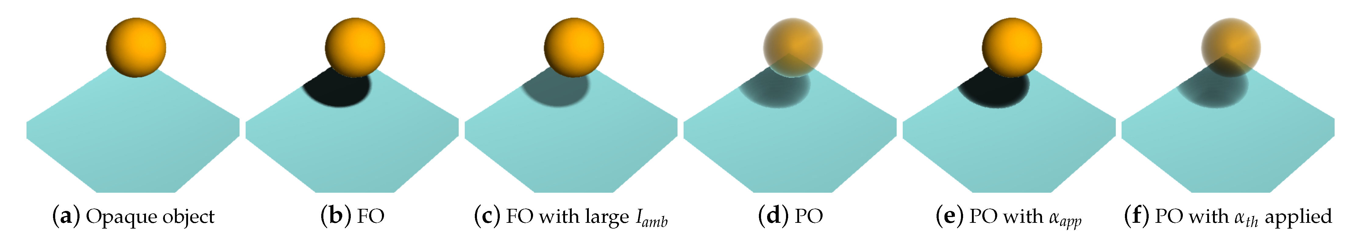
where $C_p$ is a color at a pixel from the color buffer assuming that the color of the light source is white and $I_L$ is the light intensity. $I_{\mathit{amb}}$ is an ambient light term that adjusts the darkness of the occlusion and prevents completely dark pixels. An example of full occlusion is presented in Figure 5b. The effect of large $I_{\mathit{amb}}$ is shown in (c).

3.3.2. Partial Occlusion

For partial occlusion, we could use an opacity buffer in addition to the depth buffer in order to compute how much the light intensity is transported through a transparent medium, similarly to the front-to-back ray-casting computation starting the ray marching from a pixel P. This additional opacity buffer is not necessary if we use the opacity approximation, which is introduced in Section 3.5, since there is only one parameter required per pixel and it can be stored in the A component of the color buffer (RGBA). Once the ray hit a transparent medium, we accumulated the amount of occlusion for the $i\mathrm{th}$ light sample as follows.

$${O_{\mathit{cc}}}_i=(1-{O_{\mathit{cc}}}_i)·{\alpha }_t+{O_{\mathit{cc}}}_i,$$

(4)

where ${\alpha }_t$ is the opacity value at $r\left(t\right)$ and ${O_{\mathit{cc}}}_i$ is initialized as zero. We stored multiple depth values per pixel in the depth buffers to handle transparent layers. In this paper, we used four front-most depth layers since our main interest lied between the front transparent layer and the back opaque layer. More detail about the multiple depth layers is described in Section 3.6. The termination conditions for the ray marching were: (i) $r\left(t\right)$ in Equation (1) was not placed between $(0,0,0)$ and $(1,1,1)$; (ii) ${O_{cc}}_i$ was one; and (iii) t was one. The total occlusion from N light samples was computed as follows.

$$O_{\mathit{cc}}=\frac{{\sum }_i{O_{\mathit{cc}}}_i}{N}.$$

(5)

The final color was computed using Equation (3). Figure 5d presents an example of partial occlusion. The occlusion was computed on the front layer in the example; therefore, the occlusion was not visible behind the transparent object.

3.4. Shadow and Ambient Occlusion

In Section 3.2, we present our light source model, which was defined as a disk with a radius d. The light was placed on a hemisphere with a radius R, as illustrated in Figure 1a. This model allowed us to simulate different shading effects, such as shadow and ambient occlusion. In Figure 1b, point and area lights are presented according to the light source radius d. The point light source was used to generate hard shadows, since there was only one path from a pixel to the light sample. In this case, N was one, and $N_o$ was either zero or one in Equation (2). The area light produced a soft shadow where the intensity of the soft shadow was computed by the occlusion in Equation (2) or Equation (5). Note that generally smaller d generate more hard shadows. Moreover, we could simulate ambient occlusion by choosing a large d and small R and placing the light at $\varphi =\pi /2$. This is illustrated in Figure 1c, which shows that we could produce similar conditions as in previous image-space ambient occlusion approaches, such as the image-space horizon-based ambient occlusion [5]. Figure 6 shows the different light sources applied to the engine block data. Only local illumination is used in (a), and our ISMOS model is applied in (b–d) as hard shadow, soft shadow, and ambient occlusion, respectively. (e) is a comparison image generated using the image-space horizon-based ambient occlusion [5].

3.5. Opacity Approximation

The partial occlusion computation described in Section 3.3.2 requires opacity values to accumulate the amount of light transported onto a pixel. In this section, we describe how to approximate opacity values continuously using volume transmittance.

Volume transmittance per pixel from an eye position during the ray-casting rendering was calculated as follows.

$$T\left(z\right)=exp\left(-{\int }_0^z\alpha \left(z^{\prime }\right)d{z}^{\prime }\right)$$

(6)

$$T_n\approx \prod _{j=1}^{n}exp\left(-\alpha \left(z_j\right)\Delta z\right),$$

(7)

where n is the number of samples to reach the depth z during the ray-casting rendering, $\Delta z$ the distance ($z_j-z_{j-1}$) between samples, and $\alpha$ the opacity at a certain depth z. The volume transmittance $T\left(z\right)$ is a continuous analytical form, whereas $T_n$ is a discrete form, which was used for the actual computation. The transmittance through objects is illustrated in Figure 2a and decreases as a ray passes an object. In previous work [34], a list of transmittances and their corresponding depths from a light position was stored for the deep shadow maps. To reduce the number of samples in the list, they introduced a compression scheme with an error tolerance, which is acceptable in practice. However, the compression procedure required a large storage for the list, and it might not be interactive when the light position changes. Instead, we proposed a functional approximation for the transmittance list. Figure 7a shows a graph of the transmittance as an example where the shape of the graph is similar to that of the Gaussian function. In practice, we do not need very accurate transmittance. The Gaussian function used in this work was defined as follows.

$$f\left(z\right)=exp\left(-\beta z^2\right),$$

(8)

where $\beta$ is the parameter to be approximated. Note that we used $f\left(z\right)$ to minimize the number of parameters that should be stored in a buffer, but other functional forms with more parameters can be used to approximate the transmittance more accurately. Since we wanted to find the best $\beta$ to approximate $T\left(z\right)$, we used least-squares fitting. The squared residual was defined as follows.

$$R_{\mathit{esidual}}=\sum _i{\left(\beta z_i^2-log\left(\frac{1}{T_i}\right)\right)}^2.$$

(9)

From this, we could define $X={\left(z_1^2,z_2^2,\dots ,z_n^2\right)}^T$ and $y={\left(log(1/T_1),log(1/T_2),\dots ,log(1/T_n)\right)}^T$. Then, we simply applied linear least-squares fitting. Therefore, the best $\beta$ per pixel was computed as:

$$\beta ={\left(X^{T}X\right)}^{-1}{X}^{T}y.$$

(10)

$\beta$ was computed in real time during the ray-casting rendering. The approximate transmittance $f\left(z\right)$ per pixel is shown in Figure 7b. Since we approximated the volume transmittance by only one parameter $\beta$ per pixel, $\beta$ was stored in the A component of the color buffer (RGBA) to represent the entire volume transmittance instead of using additional buffers to store opacity values corresponding to the depth layers. Note that the A component in the color buffer (RGBA) was not actually used as a color in our ISMOS model, since we did not use any blending after the first rendering pass; therefore, it was possible to use the A component for the approximation parameter $\beta$ without using an additional buffer.

To calculate the approximate opacity value at a certain z from the transmittance approximation, we used Equations (11) and (12) in the following equations.

$$\frac{f\left(z\right)}{f(z-\Delta z)}=\frac{T_n}{T_{n-1}}=exp\left(-\alpha \left(z\right)\Delta z\right).$$

(11)

Therefore, the approximate opacity was computed as:

$${\alpha }_{\mathit{app}}\left(z\right)=\frac{1}{\Delta z}·log\left(\frac{f(z-\Delta z)}{f\left(z\right)}\right).$$

(12)

This allowed us to easily and simply encode and decode the opacity values at any depth (z) position. As shown in Figure 2c, the opacity values were interactively calculated during the ray marching. We used this opacity approximation in Figure 5e with the partial occlusion computation. Note that extending our opacity approximation caused by the wavelength was possible by storing the wavelength information in an additional buffer.

3.6. Multiple Layers with Transparent Volume

We often render volumetric datasets with several transparent and opaque layers according to important features. In previous studies, the occlusion shading was applied to the entire volume. However, it was still difficult to see the shading effects on the transparent layers. Since our method operated in the image-space, applying our model to multiple layers was not easy with only one depth value per pixel. However, it was possible to find multiple layers depending on a layer differentiation method since we were using ray casting for rendering. In this work, we differentiated layers according to the transfer function settings. Note that depth peeling could be used to find multiple layers for polygonal rendering. Depth values for the layers were stored in depth buffers. The corresponding opacity values were calculated on-the-fly using our opacity approximation approach introduced in Section 3.5. We stored four front-most layers in the depth buffer as RGBA components, but it could be extended easily for more layers using more buffers. The multiple layers are illustrated in Figure 7c,d. In Figure 7c, we applied partial occlusion for pixels (d3 in the figure) on layers whose opacities ($\alpha$s) were higher than ${\alpha }_{\mathit{th}}$. For transparent pixels (d1 in the figure), we used local illumination only, such as Phong shading. The example shown in Figure 5f gave us an idea that our shading model was applied only on the opaque blue surface. We can see the shade through the transparent object (orange ball). The occlusion was computed using Equations (4) and (5).

However, applying our shading model only on opaque layers might produce unnatural effects. Instead, we computed occlusions on all layers and blended them. Figure 7d, for example, shows three layers (d1, d2, d3). d1 is not occluded, whereas d2 and d3 are partially and fully occluded, respectively. Therefore, ${O_{\mathit{cc}}}_1$ for d1 is 0, ${O_{\mathit{cc}}}_2$ is between 0 and 1, and ${O_{\mathit{cc}}}_3$ is 1. Once occlusions for all layers were calculated, we simply applied the alpha blending technique for the final occlusion, $O_{\mathit{cc}}$ from the front layer (d1) to the back layer (d3). One disadvantage was that the partial occlusion computation had to be repeated for the number of layers, but the overhead was not significant.

3.7. Multiple Directional Light Sources and Spotlight

We introduced our image-space shading model with a single light source in the previous sections. Since we just needed to compute the occlusion factor $O_{\mathit{cc}}$ in Equations (2) and (5), it was straightforward to extend the idea to multiple directional light sources. We defined full occlusion in this work as:

$$O_{\mathit{cc}}=\left(\sum _j{N_o}_j\right)/\left(\sum _j{N}_j\right),$$

(13)

where ${N_o}_j$ is the number of occluded samples from the $j\mathrm{th}$ light source and $N_j$ the total number of light samples on the $j\mathrm{th}$ light source. Similarly, partial occlusion was defined as:

$$O_{\mathit{cc}}=\left(\sum _j{\left(\sum _i{O_{cc}}_i\right)}_j\right)/\left(\sum _j{N}_j\right).$$

(14)

We then blended the colors of all light sources and applied the occlusion similarly to Equation (3). Figure 8a presents an example with two light sources for the full occlusion case. The figure shows an example with two light sources $L0$ and $L1$. From a pixel P, there were four light samples on $L0$ and five light samples on $L1$. Three out of four samples were occluded for $L0$, and two out of five were occluded for $L1$. Then, we computed the occlusion from the two light sources as $O_{\mathit{cc}}=(3+2)/(4+5)=0.555$. Let us assume that the colors for the two light sources are $C_0$ and $C_1$ and the intensities from the two lights are $I_{L0}$ and $I_{L1}$. The final color at the pixel P was computed as:

$$C_{\mathit{final}}=\frac{1}{2}·C_p·\left(C_0·I_{L0}+C_1·I_{L1}\right)·(1-O_{\mathit{cc}}),$$

(15)

where $C_p$ is the color at the pixel P from the color buffer, and we ignored the $I_{\mathit{amb}}$ term for simplicity. Note that the number of light sources was not limited to two, although we used only two light sources for the demonstration. Figure 8 shows the effect of our multiple directional light sources using a teddy bear dataset. The ambient occlusion in (c) provides good depth cues compared to the local illumination in (b). However, it is still difficult to locate the arms in (c). The red and blue lights are applied separately in (d) and (e), and they provide more visual cues around the arms in each direction. (f) presents the effect of the two lights applied together, by which the visual cues are further enhanced. This multiple directional light effect could not be easily generated by previous image-space illumination models since the occlusion was computed at each pixel with light coming from all directions on the hemisphere. Note that the same lights used in (d) and (e) are applied in (f), and the two light colors are blended using Equation (15). Due to the light intensities, two different colors are blended gradually.

A spotlight can be used to emphasize a certain area. Since we had multidirectional occlusion settings, it was easy to model a spotlight. Figure 11e illustrates our spotlight model. The model was a cone with parameters, a spotting point (C) and a covering angle ($\omega$) from a light sample ($L_p$). We tested whether a pixel (P) was within a cone by comparing the angle $\gamma$ with $\omega$ (see Figure 11e for $\gamma$ and $\omega$). $\gamma$ was calculated as $arccos\left(\frac{(P-L_p)·(C-L_p)}{\parallel P-L_p\parallel ·\parallel C-L_p\parallel }\right)$. If $\gamma$ was smaller than $\omega$, then we computed the occlusions described in the previous sections. Otherwise, the pixel was occluded without further computations, and the color at the pixel was computed as follows.

$$C_{\mathit{final}}=C_p·I_L·I_{\mathit{amb}},$$

(16)

where we assumed that the color of the light source was white.

4. Results and Discussion

We tested our approximate image-space multidirectional occlusion shading model on a Xeon CPU 2.66 GHz processor with NVidia GeForce GTX 295 graphics hardware, and for the volume rendering, we extended the ray-casting technique using the NVidia Cg shader. The color and depth from the volume rendering were stored in floating point textures, and they were used in our shading model, as described in Section 3. For the rendering without transparency, we used only one component in the depth texture; however, for the transparent object occlusion or multiple layer rendering, we used four components in the depth texture. As described in Section 3.5, the approximated opacity was easily computed using a parameter ($\beta$), which was stored together in the color buffer. Therefore, an additional opacity buffer was not required.

In the light model implementation presented in Section 3.2, the actual light samples were obtained by rotating samples on a disk with the radius r, whose center was at $(R+0.5,0.5,0.0)$, to simplify the calculations. We rotated the samples by an angle $\varphi$ about the y-axis ($R_y\left(\varphi \right)$) and then rotated them once more by an angle $\theta$ about the z-axis ($R_z\left(\theta \right)$). The rotation matrix was obtained as follows.

$$R_z\left(\theta \right)R_y\left(\varphi \right)=\left(\begin{array}{ccc}cos\left(\theta \right)cos\left(\varphi \right)& -sin\left(\theta \right)& -cos\left(\theta \right)sin\left(\varphi \right)\\ sin\left(\theta \right)cos\left(\varphi \right)& cos\left(\theta \right)& -sin\left(\theta \right)sin\left(\varphi \right)\\ sin\left(\varphi \right)& 0& cos\left(\varphi \right)\end{array}\right),$$

where $0\leqq \theta \leqq 2\pi$ and $0\leqq \varphi \leqq \pi$.

We used six different datasets to show the effects of our ISMOS model, as summarized in

Table 1. Performance in fps. “1 L” means one light source, and “2 Ls” indicates two light sources. “FO” is full occlusion, and “PO” is partial occlusion. “PO, 1” indicates PO with one layer, and “PO, m” is PO with m layers. “${\alpha }_{\mathit{app}}$” means that the opacity approximation is used in the column.

Dataset	Size	Local Illumination	1 L, FO	1 L, PO, 1	1 L, PO, m	1 L, PO, 1, ${\mathit{\alpha }}_{\mathit{app}}$	1 L, PO, m, ${\mathit{\alpha }}_{\mathit{app}}$	2 Ls, FO	2 Ls, PO, 1	2 Ls, PO, m	2 Ls, PO, 1, ${\mathit{\alpha }}_{\mathit{app}}$	2 Ls, PO, m, ${\mathit{\alpha }}_{\mathit{app}}$
Engine	$256\times 256\times 128$	23.3	19.7	15.8	13.4	12.1	11.2	16.1	13.6	12.5	10.1	9.2
Teddy bear	$512\times 512\times 63$	22.7	18.5	15.1	13.1	13.8	12.5	15.3	12.1	8.8	9.1	8.6
Head	$256\times 256\times 225$	22.2	19.6	16.1	10.2	11.0	8.3	18.1	15.3	8.1	8.9	6.9
Abdomen	$256\times 256\times 128$	20.0	13.5	11.2	10.8	8.9	7.5	11.4	9.7	8.6	7.9	7.0
Carp	$256\times 256\times 512$	20.8	14.1	13.3	12.7	12.1	11.8	12.1	11.9	11.1	9.5	8.8
Stag beetle	$832\times 832\times 494$	10.4	9.2	8.2	7.9	7.5	6.9	7.8	6.4	6.0	5.5	5.1

. The engine data are presented with different shading methods in Figure 6. Our ISMOS model was able to produce the different shading effects by simply adjusting the light parameters. The shadow (b,c) and ambient occlusion (d) provided more depth cues compared to simple local illumination (a). The ambient occlusion effect (d) from our ISMOS was similar to the effect (e) proposed by Bavoil et al. [5]. Figure 8 presents the effect of the multiple directional light sources applied to the teddy bear dataset. The two directional lights in (f) provide more visual cues compared to the previous ambient occlusion method (c) and shading with a single light source (d,e).

We show an occlusion caused by transparent layers on an opaque layer in Figure 9. The transparent skin occludes the light arriving on the bone, and the effect is shown in (b) and (c). The occlusion is also caused by the bone, and this is seen around the back side of the neck bone. As seen in the figure, less light on the bone is observed in (c) compared to (b) since the more opaque skin in (c) occludes the light arriving at the bone more than the more transparent skin in (b). The occlusions on multiple layers are computed and blended in (d).

The abdomen data are compared with different shading methods in Figure 10. The data were rendered with the opaque transfer function setting in (a–c) and transparent setting in (d–f). (c) shows the full occlusion of ISMOS and provides very good depth cues compared to (a) and (b). We also compare the multiple layer effect in (e) and (f), and a part of the scene is highlighted with a blue box. The shading is visible through the transparent object, and the multilayer occlusion shows more natural shading effect as seen in (f). The carp data were used to show how well our ISMOS worked on a complicated structure in Figure 11. We extracted a bone structure out of the data and applied ISMOS on it. The opacity approximation is applied in (c,d), and we can see that the approximation is very reliable to represent the bone structure. Furthermore, the spotlight is used in (d), which enables us to focus on a certain area and to reduce the computation time since scenes outside the spotlight are simply occluded. Our ISMOS model in (c,d) provides proper visual cues of the object compared to (a,b). Similar effects are obtained with the beetle data as presented in Figure 12. We compare the accuracy of the opacity approximation in (c) and (d); and (f) and (g). Furthermore, we can see more natural shading effects with the multiple layer occlusion, and they are shown in (h) compared to (g). Moreover, the perceptual cue is improved with our ISMOS.

For the performance measurement, we used ray casting with a $580\times 580$ view port in the volume rendering. The performances are summarized in Table 1. As shown in the table, the performance overhead was similar for all datasets. An average 13.8 ms overhead was measured for full occlusion with one light source and an average 25.6 ms overhead with two light sources. The average performance difference between the full and partial occlusion was about 11.4 ms, and the opacity approximation required on average 15.9 ms. The number of light sources affected the performance, but the difference was fairly small. Note that our focus was not the optimization of the ray casting volume rendering, but the overhead for our shading model. Therefore, our performance on the volume rendering might not be faster compared to other highly optimized volume renderings, but the overhead was the same all the time as long as the view port size was fixed. Although there was a performance overhead by applying our ISMOS model, we still obtained interactive performance for all datasets even with transfer function changes and light source changes.

For the quality comparison, we compare our hard shadow with the existing deep shadow map [27] in Figure 13. Local illumination in (a), ambient occlusion in (b), deep shadow map in (c), and our hard shadow by ISMOS in (d) are compared. As seen in the figure, our hard shadow is almost identical to the deep shadow map. Although our model supported various lighting models, indirect lighting was not achieved since indirect lighting was not interpreted within the model. However, it was possible to extend our model to support the enclosed volume with a partially opaque object and multiple objects with varying partial opacity by adding more buffers to store more precise transmittance.

5. Conclusions and Future Work

In this work, we presented a novel approximate image-space multidirectional occlusion shading model for volume rendering. Our model was a unified shading model to simulate different light sources, and it provided more visual cues with minor performance overhead compared to using only local illumination. The occlusion for the opaque and transparent medium was handled separately using the full and partial occlusion methods. Our model caused small overhead in texture memory compared to the previous techniques and did not require any preprocessing. The transfer function and light position could be changed interactively. Moreover, we introduced an opacity approximation that allowed us to compute opacity values at any depth z instead of using additional opacity buffers. In order to produce a more natural shading effect, we blended the occlusion shadings from multiple layers, and we were able to produce realistic shading results through a transparent volume. Multiple directional light sources enhanced visual cues more with a small overhead. Then, we tested our ISMOS model with various datasets and proved that the ISMOS provided better visual cues with a small amount of additional computation. Our model can be applied to any rendering system since the ISMOS is decoupled from the rendering pass. As future work, we will optimize the ISMOS computation. Since the light source can be located anywhere in a volume, we will study an efficient image-space subsurface scattering effect. Moreover, we will investigate more efficient layer management to handle more layers in the future.