Linear and Nonlinear Normal Interface Stiffness in Dry Rough Surface Contact Measured Using Longitudinal Ultrasonic Waves

Abstract

When two rough surfaces are loaded together contact occurs at asperity peaks. An interface of solid contact regions and air gaps is formed that is less stiff than the bulk material. The stiffness of a structure thus depends on the interface conditions; this is particularly critical when high stiffness is required, for example in precision systems such as machine tool spindles. The rough surface interface can be modelled as a distributed spring. For small deformation, the spring can be assumed to be linear; whilst for large deformations the spring gets stiffer as the amount of solid contact increases. One method to measure the spring stiffness, both the linear and nonlinear aspect, is by the reflection of ultrasound. An ultrasonic wave causes a perturbation of the contact and the reflection depends on the stiffness of the interface. In most conventional applications, the ultrasonic wave is low power, deformation is small and entirely elastic, and the linear stiffness is measured. However, if a high-powered ultrasonic wave is used, this changes the geometry of the contact and induces nonlinear response. In previous studies through transmission methods were used to measure the nonlinear interfacial stiffness. This approach is inconvenient for the study of machine elements where only one side of the interface is accessible. In this study a reflection method is undertaken, and the results are compared to existing experimental work with through transmission. The variation of both linear and nonlinear interfacial stiffnesses was measured as the nominal contact pressure was increased. In both cases interfacial stiffness was expressed as nonlinear differential equations and solved to deduce the contact pressure-relative surface approach relationships. The relationships derived from linear and nonlinear measurements were similar, indicating the validity of the presented methods.

1. Introduction

When two solid surfaces come into contact, it is the asperity peaks that touch, and the real area of contact is substantially less than the nominal contact area [1]. Applying a pressure to the surfaces causes a small approach of the mean lines of their roughness. The interfacial stiffness (per unit area) is then defined as the rate of change of contact pressure with approach of the mean lines of the roughness of the contacting surfaces [2]. If the real contact area is low, then a low nominal contact pressure is all that is required to deflect the asperities. Increasing the nominal contact pressure brings more asperities into contact and the interface becomes stiffer; hence interface stiffness is a nonlinear variable. Interfacial stiffness is important in tribology because it affects machine element deflection, wear, and friction, since stiffer interfaces tend to less deflection. Machining accuracy, for example, depends on the stiffness of the joints in the machine tool assembly [2].

Several studies have focused on the interfacial stiffness of rough contact from both theoretical and experimental perspectives. An early example from Mindlin [3] provided a theoretical model for elastic contact of a smooth curved surface. Later, Greenwood and Williamson (GW model) [4] presented a statistical model for the relation between the contact area of the rough elastic mating surfaces and applied pressure. The model is limited by two assumptions: firstly asperities are treated as a distribution of hemispherical capped peaks, and secondly those peaks are treated as independent such that the deformation of one peak does not affect its neighbors. The relationship between the contact area and applied pressure also presented by models such as the Whitehouse-Archard-Onion model (WAO model) [5,6] and the Buh-Gibson-Thomas model (BGT model) [7]. These models have been widely used to predict contact stiffness. Campana et al. [8] used Mindlin’s theory to measure the stiffness ratio of stationary contact.

Digital image correlation (DIC) [9,10,11] has been used to measure stiffness in joints. In this method, a series of images prior to applying load and during loading are taken from the interface and surrounding area. The comparison of the images shows the relative displacement. A plot of the applied load measured with a load cell against the relative surface displacement is created; the gradient gives the contact interface. Although it has advantages such as a full field capability and high resolution, the main limitation is that a surface near the contacting surfaces must be accessible for the camera to capture images. In many items of engineering machinery optical access is limited and this limits application of DIC outside a laboratory setting. Another method is to make direct measurements of the displacement of the interface under applied load. Burdekin et al. [12] used relative displacement transducers between the fixed frame and the stack of rings to measure direct displacement of the interface. Chikate et al. [13] also directly measured displacement of a smooth surface using strain gauges and spring-loaded pins. For example, Handzel-Powierza et al. [14] used a tenso-metric bridge to measure the applied load and an indicator sensor to measure the surface approach. They compared their results to theoretical predictions from the Greenwood-Williamson model in the range of elastic deformation for quasi-isotropic surfaces. However, this technique is restricted to low contact stiffness $\left(1 \mathrm{GPa}/\mathsf{\mu }\mathrm{m}\right)$ [15].

It is also possible to measure contact stiffness from a structure’s resonance frequency. This contact frequency method uses a relationship between the contact stiffness and the natural frequency of the mating surfaces [16]. One of the disadvantages of this method is the need for vibration response equations of the experimental tools [17].

The approach used here, also a vibrational method, is through the reflection or transmission of ultrasound [11,18,19,20,21,22,23]. This has the advantage being non-invasive, non-destructive, and can measure interface inside a machine where desired surfaces are inaccessible. Reflection and transmission coefficients are defined as the proportion of an incident wave reflected from or transmitted through the interface, respectively. The reflection coefficient depends on the amount of solid contact. The acoustic impedance of air is significantly small, compared to solid materials, and so the air gap at the interface causes more incident energy to reflect. Increasing the nominal contact pressure leads to an increase in the number of the asperities in contact, therefore less incident energy is reflected and more energy transmitted [18]. Kendal and Tabor [24] and Tattersall [19] used a spring model, where the interface is treated as a distributed stiffness, to demonstrate that the reflection coefficient of an imperfect contact (incomplete contact) is dependent on the interfacial stiffness.

Authors have studied both normal and tangential interface stiffness in the linear regime using either longitudinal or transverse polarised ultrasound, respectively [11,18,19,20,21,22,23,25,26,27]. Both elastic and plastic rough surface contact models have been used to predict interface stiffness compared to ultrasonic measurement [15,28,29].

Krolikowski et al. [15,28] presented a spring-damper model in a parallel configuration to address the effect of ultrasound attenuation. However, the results were still far beyond those predicted by the GW model. Rokhlin et al. [30] modeled the interface as a layer of equivalent materials such as viscoelastic materials. Their study is accurate in cases where the Poisson’s ratio of the layer model is known. The principle has been modified by Du. et al. [31], Xiao et al. [32] and Sun et al. [17].

These studies have been based around the linear response of an interface to an ultrasonic wave. The pressures generated by the wave and the resulting deflections are normally very small and so the process is elastic and reversible. However, in recent years there have been a number of studies based around higher power ultrasound that causes nonlinear behaviour. The nonlinear behaviour may originate from the material itself, as the stress-strain relationship of the medium exceeds Hooke’s law (nonlinear elasticity) [33,34]. Alternatively, the interface may also be a source of nonlinearity. If the wave is of sufficient power, it can cause opening and closing of the air gaps and this can lead to the generation of higher harmonics in the reflected/transmitted waves. This is known as Contact Acoustic Nonlinearity CAN [35,36,37]. In Section 2, a description of the higher harmonics generation (mechanics of CAN) is described.

Richardson [38] studied one-dimensional nonlinear wave propagation through identical contacting materials by considering the concept of CAN. He defined an analytical relation between the incident wave and the relative surface approach of the interface. Biwa et al. [39] used Richardson’s findings to propose a nonlinear nominal contact pressure-relative surface approach relationship using a polynomial Taylor series to define the linear and nonlinear interfacial stiffnesses using the reflection coefficient. Nonlinear interfacial stiffness is important when a high-power ultrasound is employed to define the interface. The wave itself causes a distortion of the interface and hence a linear model can no longer describe the proper interface response. In previous studies only through transmission methods had been used to measure the nonlinear interfacial stiffness. The aim of this paper is to evaluate linear and nonlinear interfacial stiffnesses measured with a reflection method to demonstrate that they are both based on the same fundamental relationship between contact pressure and relative surface approach. The result is compared to published experimental work using through transmission.

Both the linear and nonlinear interfacial stiffness have been deduced using a reflection coefficient R and a second order nonlinear parameter for reflected ultrasound from the interface γ. A fourth-order polynomial expression for the linear and nonlinear interfacial stiffness variation with nominal contact pressure based on experimental data is used. Since the accuracy of the nonlinear stiffness measured with ultrasound has not been studied, a first order nonlinear homogenous differential equation of the linear interfacial stiffness and a second order nonlinear homogenous differential equation of the nonlinear interfacial stiffness have been used to derive the relationship between nominal contact pressure and approach of the surface. The study shows the nominal contact pressure–relative surface approach measured from the linear and nonlinear interfacial stiffness both give similar results. This indicates the equations proposed by [39] for the linear and nonlinear interfacial stiffness can accurately measure the interfacial stiffness.

2. Theoretical Approach

2.1. Governing Equation

Consider two linear elastic media in contact subjected to a one-dimensional elastic longitudinal ultrasonic wave (Figure 1).

The direction of ultrasound propagation is through the thickness of the media which is defined as the $x$-axis. The origin of the $x$-axis is the point of first contact of the surfaces. The roughness mean lines above and below the interface are located at $X_{-}$ and $X_{+,}$ respectively (Figure 1a). The separation (mean gap) between the two surfaces under zero load is then given by ($X_{+}-X_{-}$). When there is no elastic wave the surfaces are in static equilibrium under a nominal contact pressure $p_0$ causing an equilibrium separation of $h_0$ (Figure 1b,c). When an elastic wave passes through the interface the surface separation, $h\left(t\right)$ is cyclically reduced and then increased about the equilibrium value $h_0$. The relative surface approach $Y\left(t\right)$ is defined as the difference between the separation variation with time $h\left(t\right)$ and equilibrium separation $h_0$, $\left(Y\left(t\right)=h\left(t\right)-h_0\right)$. In the absence of an elastic wave, the relative surface approach$Y\left(t\right)$ is zero. The sign of relative surface approach $Y\left(t\right)$ is opposite to the direction of loading/unloading by the wave. During the loading process by the elastic wave, the relative surface approach $Y\left(t\right)$ is negative, whereas during the unloading process it is positive. In order to clearly illustrate the relative approach of the surfaces (assuming the lower body is fixed and the upper moving), the upper body is considered to be rigid and flat whilst the lower body is elastic and rough (Figure 1c).

The elastic wave pressure superimposed on the nominal contact pressure $p_0$ generates a relative surface approach $Y\left(t\right)$ which varies with time (shown in Figure 1d). Increasing nominal contact pressure $p_0$ decreases separation of the surfaces.

The equations described in this section follow the method presented in [38,39]. The equation of the interface subjected to a one-dimensional longitudinal ultrasonic wave is given by:

$$\rho \frac{{\partial }^{2}u}{\partial t^2}=\frac{\partial \sigma }{\partial x}$$

(1)

The stress-displacement relation is given by:

$$\sigma \left(x,t\right)+p_0=E\frac{\partial u}{\partial x}$$

(2)

where $\rho$ is the density of the media, $\sigma \left(x,t\right)$ is the normal stress generated by the ultrasonic wave and $p_0$ in the media, $u\left(x,t\right)$ is the displacement of the ultrasonic wave and $p_0$ is the nominal contact pressure. The general solution of Equation (1) results in the displacement of each side of the interface:

$$\{\begin{array}{c}u\left(x,t\right)=f\left(x-ct\right)+G\left(x+ct\right) , x{X}_{-}\\ u\left(x,t\right)=H\left(x-ct\right) , x{X}_{+}\end{array}$$

(3)

where $u\left(x,t\right)$ is the displacement of the interface, $c$is the speed of sound in the media which is $\sqrt{E/\rho }$, $t$ is the time of flight of ultrasound, $f\left(x-ct\right)$ is the incident wave, $G\left(x+ct\right)$and$H\left(x-ct\right)$ are the reflected and transmitted wave, respectively. The displacement through the upper and lower media is as $x{X}_{-}$ and $x{X}_{+},$ respectively. The boundary condition at the interface is defined by:

$$\sigma \left(X_{+},t\right)=\sigma \left(X_{-},t\right)=-p\left(h\left(t\right)\right) , p\left(h_0\right)=p_0$$

(4)

where $h\left(t\right)$ is the rough surface mean line separation (surface separation) variation with time and $h_0$ is the separation under static equilibrium $p_0$ in the absence of the elastic wave (as shown in Figure 1). A negative sign pressure term indicates compression at the interface. Substituting Equation (4) into Equation (2) gives:

$$\{ \begin{array}{c}\frac{\partial u\left(X_{-},t\right)}{\partial x}=\frac{-1}{E}p\left(h\left(t\right)\right)+\frac{1}{E}{p}_0 \\ \frac{\partial u\left(X_{+},t\right)}{\partial x}=\frac{-1}{E}p\left(h\left(t\right)\right)+\frac{1}{E}{p}_0 \end{array}$$

(5)

The relative surface approach $Y\left(t\right)$ of the mating surfaces is defined as the difference in the wave displacement $u\left(x,t\right)$ of both sides of the interface (Figure 1d):

$$Y\left(t\right)=\left\{u\left(X_{+},t\right)-u\left(X_{-},t\right)\right\}=h\left(t\right)-h_0$$

(6)

Equation (6) shows that the relative surface approach $Y\left(t\right)$ can be used instead of the surface separation $h\left(t\right).$ The translational motion of the interface is defined by:

$$X\left(t\right)=\left\{u\left(X_{+},t\right)+u\left(X_{-},t\right)\right\}/2$$

(7)

In order to simplify the calculation, the displacement of the interface is represented only in terms of incident wave [38]:

$$X\left(t\right)=f\left(x-ct\right)$$

(8)

Differentiation of Equations (6) and (8) with respect to time gives:

$$\dot{X}=\frac{-c \partial f\left(X\_-ct \right)}{\partial \left(X\_-ct\right)}$$

(9)

where dots denote the differentiation with respect to time.

$$\dot{Y}=c\left\{-\frac{ \partial H\left(X_{+}-ct\right)}{\partial \left(X_{+}-ct\right)}+\frac{ \partial f\left(X_{-}-ct\right)}{\partial \left(X_{-}-ct\right)}-\frac{ \partial G\left(X_{-}+ct\right)}{\partial \left(X_{-}+ct\right)}\right\}$$

(10)

Equation (10) is expressed in terms of incident, reflected, and transmitted ultrasonic waves; it is necessary to reduce this in terms of only the incident wave and nominal contact pressure. To do this Equation (3) is differentiated with respect to $x$:

$$\{ \begin{array}{c}\frac{\partial u\left(X_{-},t\right)}{\partial x}=\frac{\partial f\left(X_{-}-ct\right)}{\partial \left(X_{-}-ct\right)}+\frac{\partial G\left(X_{-}+ct\right)}{\partial \left(X_{-}+ct\right)} \\ \frac{\partial u\left(X_{+},t\right)}{\partial x}=\frac{\partial H\left(X_{+}-ct\right)}{\partial \left(X_{+}-ct\right)} \end{array}$$

(11)

Rearranging Equation (11) to make the reflected and transmitted waves the subject gives:

$$\{ \begin{array}{c}\frac{\partial G\left(X_{-}+ct\right)}{\partial \left(X_{-}+ct\right)}=\frac{\partial u\left(X_{-},t\right)}{\partial x}-\frac{\partial f\left(X_{-}-ct\right)}{\partial \left(X_{-}-ct\right)} \\ \frac{\partial H\left(X_{+}-ct\right)}{\partial \left(X_{+}-ct\right)}=\frac{\partial u\left(X_{+},t\right)}{\partial x} \end{array}$$

(12)

Substituting Equation (5) into Equation (12) gives:

$$\{ \begin{array}{c}\frac{\partial G\left(X_{-}+ct\right)}{\partial \left(X_{-}+ct\right)}=\frac{-1}{E}p\left(h\left(t\right)\right)+\frac{1}{E}{p}_0-\frac{\partial f\left(x-ct\right)}{\partial \left(x-ct\right)} \\ \frac{\partial H\left(X_{+}-ct\right)}{\partial \left(X_{+}-ct\right)}=\frac{-1}{E}p\left(h\left(t\right)\right)+\frac{1}{E}{p}_0 \end{array}$$

(13)

Substituting Equation (13) into Equation (10) gives:

$$\dot{Y}=2c\frac{ \partial f\left(X\_-ct\right)}{\partial \left(X\_-ct\right)}+\frac{2}{\rho c}\left\{ p\left(h_0+Y\right)-p_0\right\}$$

(14)

Equation (14) is a first order differential equation describing the relative surface approach in terms of the incident wave and the nominal contact pressure $p\left(h_0+Y\right)$. Solving this differential equation results in an equation for the relative separation of the interface. Equation (14) can be written in terms of surface separation $h\left(t\right)$:

$$\dot{h}=2c\frac{ \partial f\left(X\_-ct\right)}{\partial \left(X\_-ct\right)}+\frac{2}{\rho c}\left\{ p\left(h\right)-p_0\right\}$$

(15)

The reflected ultrasonic wave is now defined in terms of relative surface approach. Equations (5) and (6) give the relationship between relative surface approach $Y\left(t\right)$ and translational motion of the contact interface $X$:

$$u\left(X_{-},t\right)=X\left(t\right)-\frac{1}{2}Y\left(t\right)$$

(16)

Substituting Equation (3) (for $x{X}_{-})$ and Equation (7) into Equation (15) gives:

$$G\left(x+ct\right)=-\frac{1}{2}Y\left(t+\frac{x-X_{-}}{c}\right)$$

(17)

It can be seen from Equation (17) that the reflected ultrasonic wave $G\left(x+ct\right)$is expressed only in terms of the relative surface approach. The negative sign of the reflected wave indicates propagation in the opposite direction to the incident wave through the upper body.

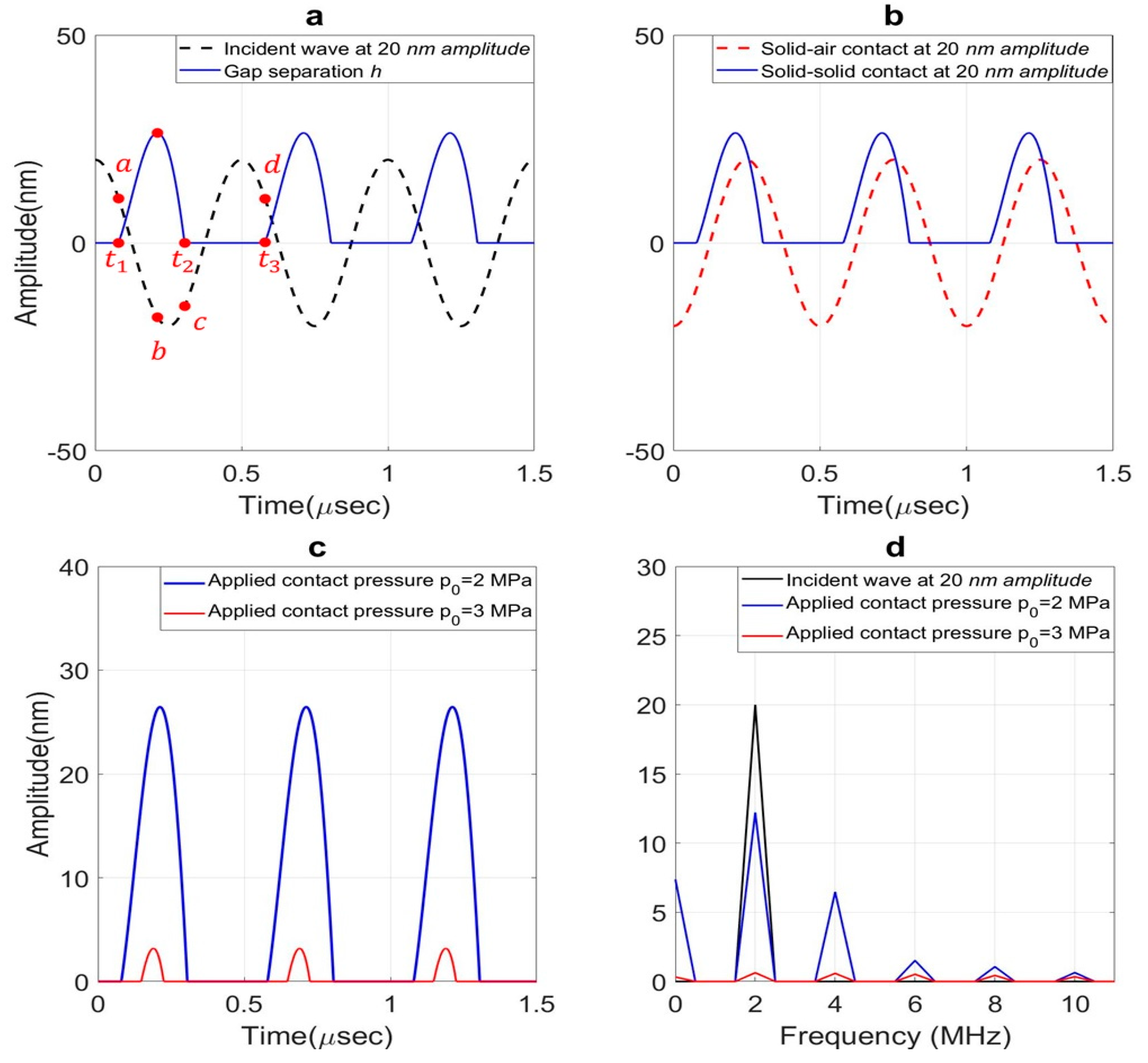
2.2. Determination of Contact Acoustic Nonlinearity (CAN)

An interface consists of asperity contacts and air gaps. In the regions of the interface with the air gap, there is no contact between the surfaces (Figure 2a). The approach of the two surfaces depends on the magnitude of the applied pressure [40]. The applied pressure is the sum of the externally applied pressure and the pressure applied by the incident wave.

A longitudinal incident cosinusoidal wave with centre angular frequency $\omega$ and amplitude $A$ strikes the interface at time $t_0$.

$$f\left(x-ct\right)=Acos\left\{\frac{\omega }{c}\left(x-X_{-}-ct\right)\right\}$$

(18)

Substituting Equation (18) into Equation (15) at the interface gives:

$$\dot{h}=2A\omega \sin \omega t+\frac{2}{\rho c}\left\{p\left(h\right)-p_0\right\}$$

(19)

It is assumed at time $t_0=0$ that the gap is closed and remains closed until just before time $t_1$. For the sake of derivation, the gap is assumed to be fully closed; however, in reality even under high pressure there will remain air gaps and the contact does not fully close. Therefore, the gap separation $h$ and relative surface separation $Y$ are zero, subsequently, the initial surface separation $h_0$ is zero. When the gap is open at time $t_1$, the pressure at the interface is zero, so the boundary condition in Equation (4) is:

$$\sigma \left(X_{+},t\right)=\sigma \left(X_{-},t\right)=-p\left(h\left(t\right)\right)=0$$

(20)

Substituting Equation (20) into Equation (19) and integrating with respect to time gives time $t_1$:

$$cos\omega t_1+\frac{p_0}{\rho cA} t_1-1=0$$

(21)

Equation (21) is different from those presented in [38]. Equation (21) is a nonlinear equation and in the present work it is solved by the Newton-Raphson method.

The gap remains open until time $t_2$. Integration of Equation (19) with respect to time and substituting Equation (20) in the interval [$t_1, t_2]$ gives opening interval:

$$h\left(t\right)-h\left(t_1\right)=-2A\left\{cos\omega t-cos\omega t_1\right\}-\frac{2}{\rho c}{p}_0\left(t-t_1\right) ; t_1\le t\le t_2$$

(22)

Hence at time $t_2$ the gap is just about to be closed; the right-hand side of Equation (21) is zero. Time $t_2$ can be found using the Newton-Raphson method:

$$cos\omega t_2+\frac{p_0}{\rho cA}{t}_2-cos\omega t_1-\frac{p_0}{\rho cA}{t}_1=0$$

(23)

The gap remains closed until time $t_3$. The opening-closing gap transition is repeated periodically:

$$h\left(t\right)=\{\begin{array}{c}h\left(t_{2n}\right) ; t_{2n}\le t{t}_1+nT\\ h\left(t_{2n}\right)-2A\left\{\cos \omega t-\cos \omega \left(t_1+nT\right)\right\}-\frac{2}{\rho c}{p}_0\left(t-t_1-nT\right); t_1+nT\le t{t}_2+nT \end{array}$$

(24)

where $n=0,1,2,\dots$ and $T$ is the period of the incident wave.

A single longitudinal incident ultrasonic wave cycle consists of two parts causing tension and compression (Figure 2b). Figure 3 shows surface separation at the interface of aluminium blocks subjected to a longitudinal wave with centre frequency $2 \mathrm{MHz}$ and amplitude $20 \mathrm{nm}$. The gap is initially assumed to be closed at time $t_0=0$. It is seen from Figure 3a that, when the compressional part of wave reaches the interface (corresponding to zero to point a on the incident wave), the applied pressure is sufficiently large to keep the gap closed in the interval [$t_0,t_1]$ (also see Figure 2c). As the wave passes (corresponding to part of the wave between point a and b on the incident wave), the applied pressure reduces so the surfaces of the gap are open at time $t_1$ and be pulled apart away from the mean position (also see Figure 2d). After that, the applied pressure increases (corresponding to part of the wave between point b and c on the incident wave) and presses the surfaces of the gap closer together.

In the time interval [$t_2,t_3]$ the gap is closed as the applied pressure increases (corresponding to part of the wave between point c and d on the incident wave). The opening-closing gap transition is repeated periodically. Figure 3b shows solid–solid contact and solid–air contact. Time domain signals presented in Figure 3b,c were converted to frequency domain using Fast Fourier Transform (FFT). It is seen that the surface of a solid-air contact freely moves, therefore no higher harmonic is generated. However, higher harmonics are generated (both even and odd) in solid–solid contact (Figure 3d). Figure 3c shows the effect of nominal contact pressure on the opening and closing the gap in the interface. It is seen that the higher nominal contact pressure closes the gap for longer period and the surfaces are separated less.

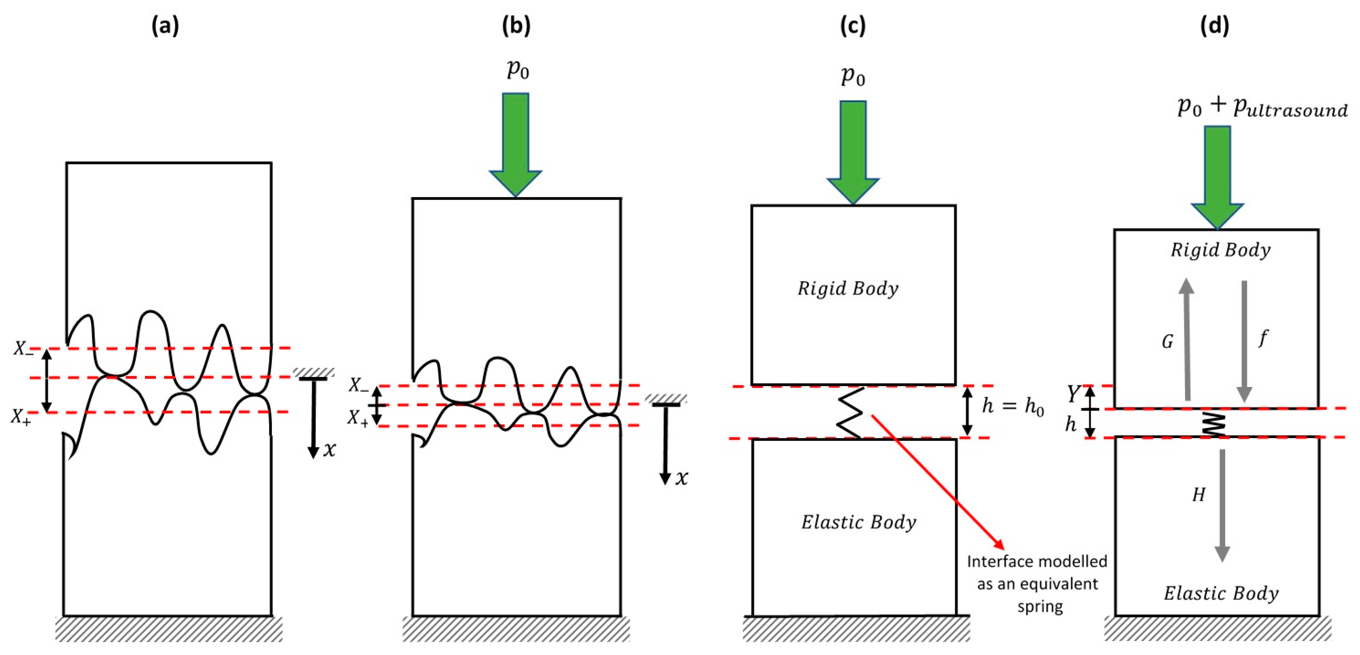
2.3. Theoretical Analysis

Evaluation of the general equations presented in Section 2.1 requires further theoretical analysis to drive the equations of interfacial stiffness.

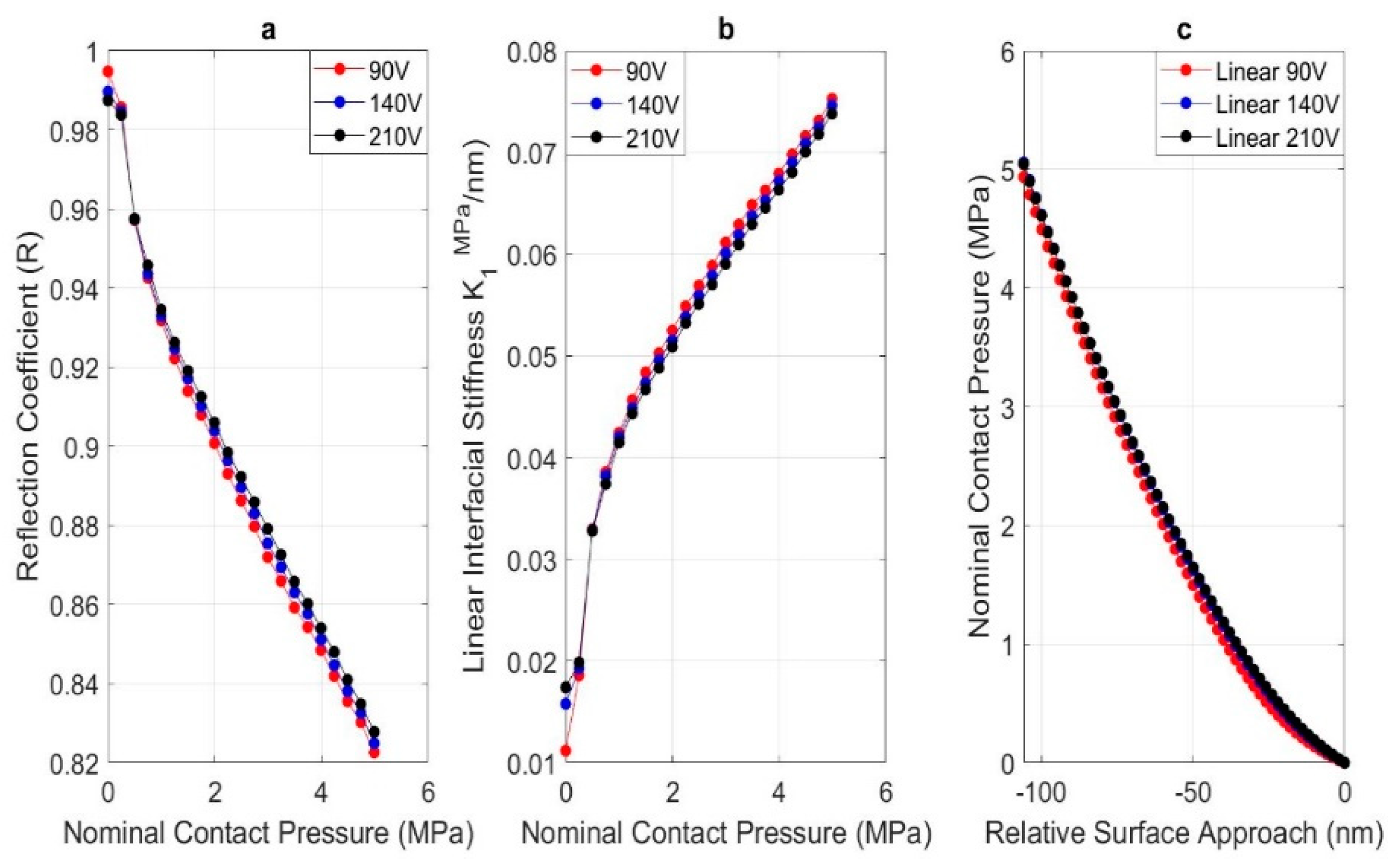
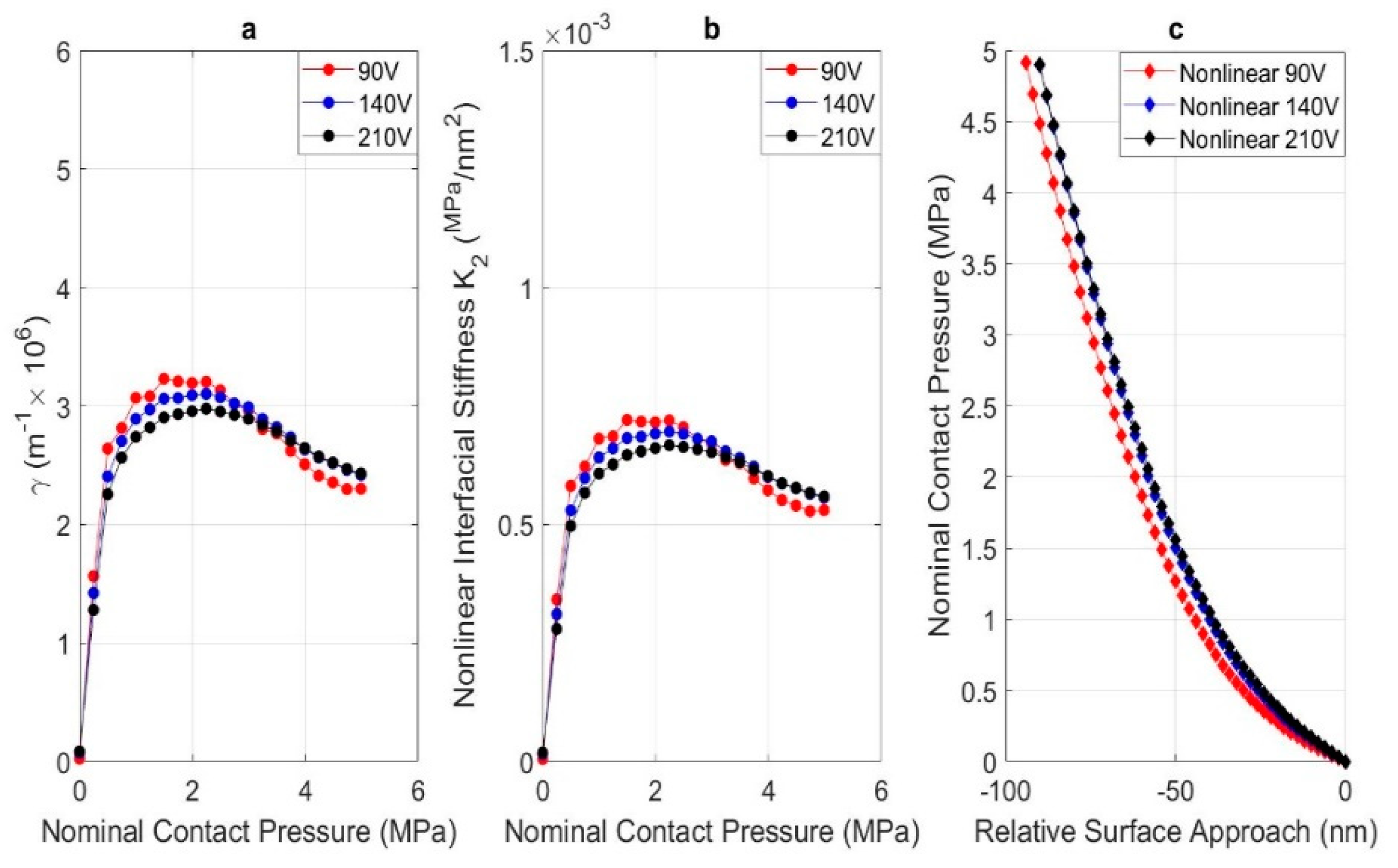
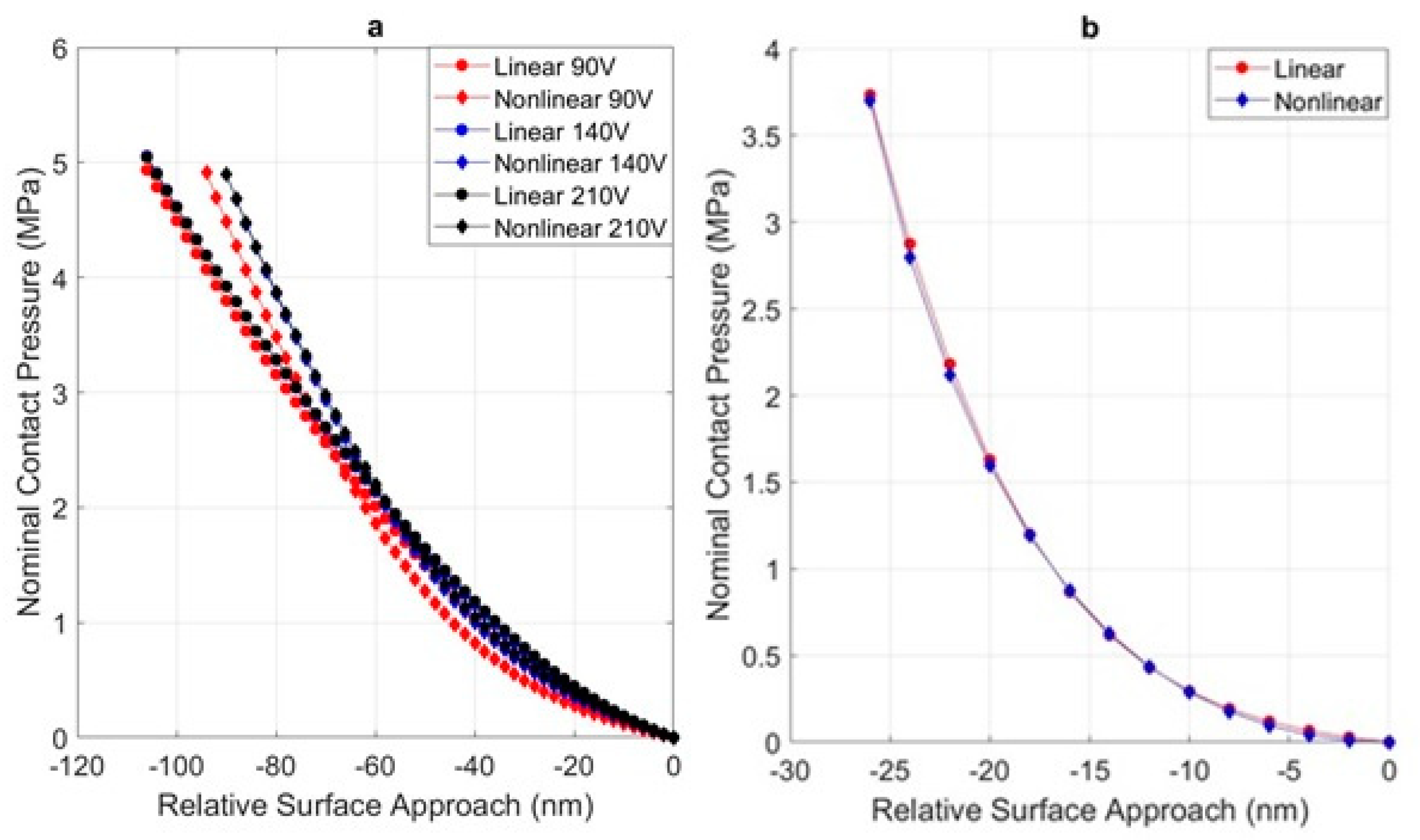
2.3.1. Linear and Nonlinear Interfacial Stiffness

The stiffness of an interface can be modelled as a series of springs created by the individual asperity contacts [20,24]. The series of the springs is then equivalent to a single distributed spring with an equivalent stiffness $K$ (expressed per unit area) [2]:

$$K=-\frac{d{p}_0}{dh}$$

(25)

For practical rough surface contacts, the spring is nonlinear since the relation between the applied pressure and surface separation is not directly proportional. As the contact pressure is increased, more asperity contact occurs and the interface becomes stiffer. If the deflection is small (and less than the elastic limit of the spring material [42]) the nonlinearity can be neglected. For large deflections, the pressure–separation relationship and the resulting nonlinear stiffness must be considered. One of the approaches to deal with the nonlinear contact pressure-relative surface approach of the interface (boundary or contact nonlinearity) is to express it as a series of polynomial terms in a Taylor series around $h=h_0$ [39]:

$$p\left(h\right)=p\left(h_0+Y\right)=p_0-K_{1}Y+K_2{Y}^2$$

(26)

where $K_1$ and $K_2$ are the linear and second order nonlinear interfacial stiffness and $p_0$ is the nominal contact pressure at $h_0$. The linear $K_1$ and nonlinear $K_2$terms of the interfacial stiffness are then defined by:

$$K_1=-\frac{dp}{dY} , h=h_0$$

(27)

$$K_2=\frac{1}{2}\frac{d^{2}p}{d{Y}^2} , h=h_0$$

(28)

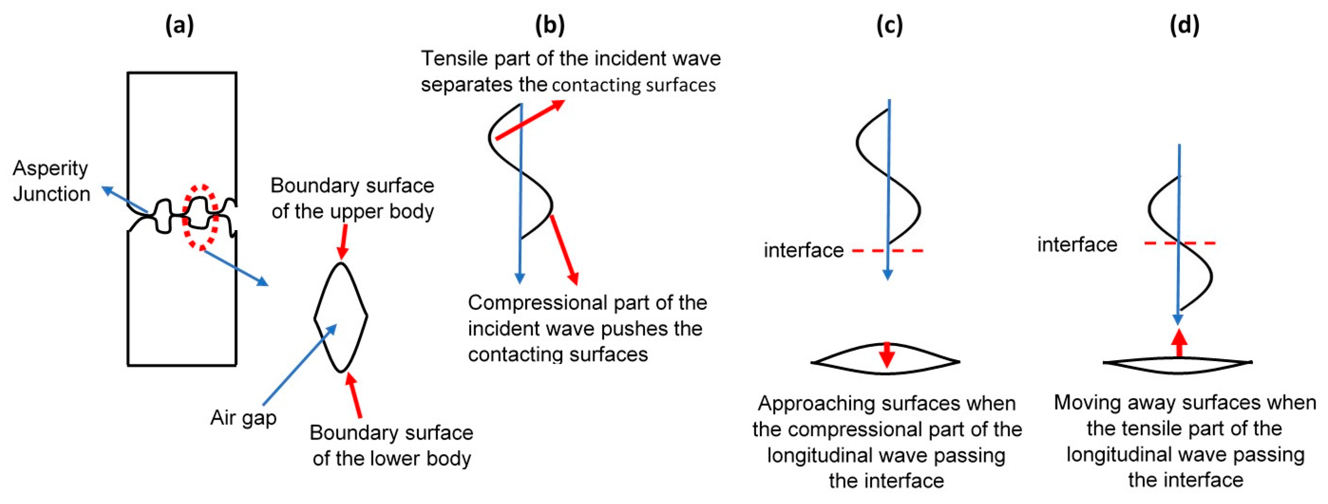
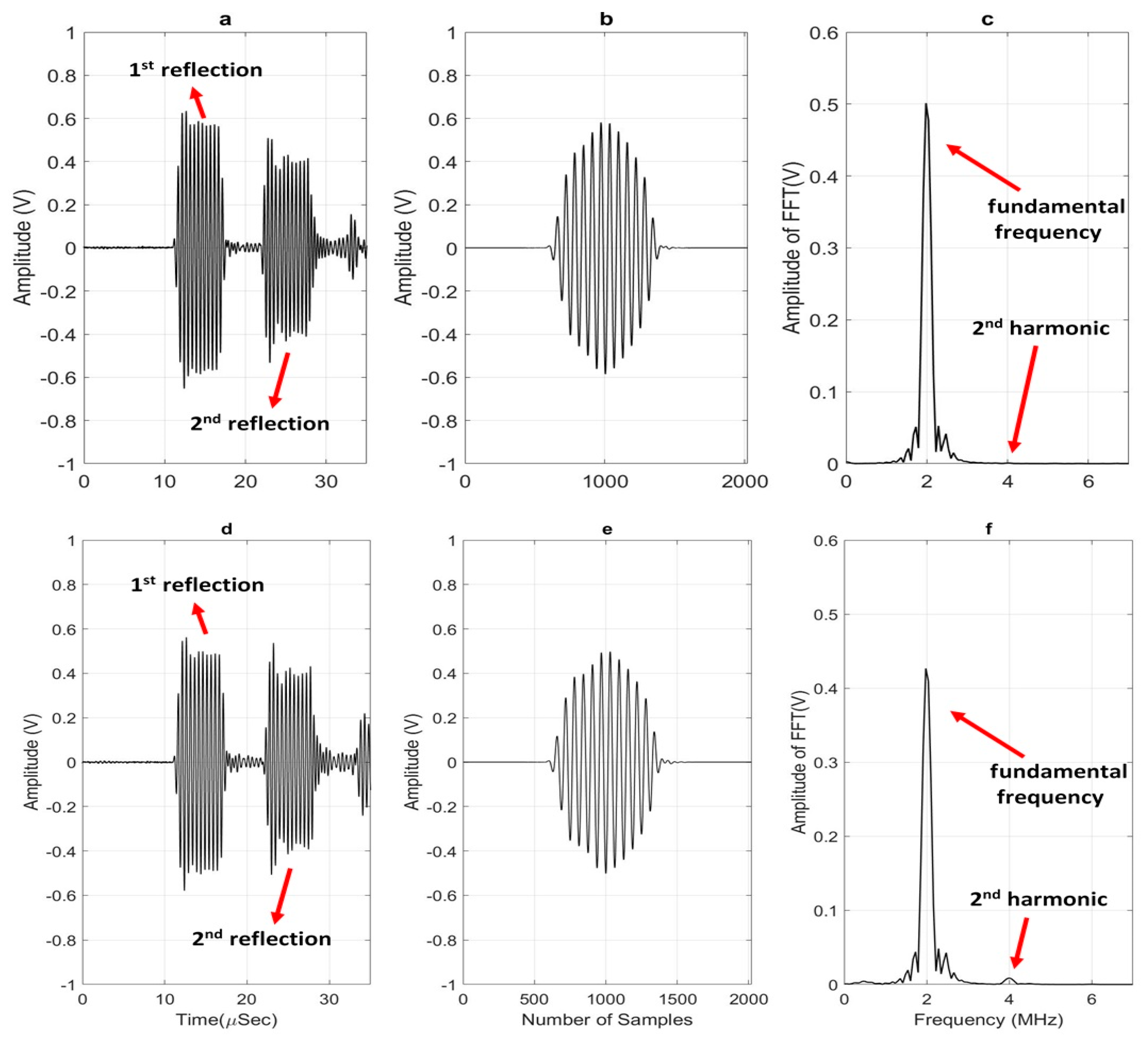
2.3.2. Incident and Reflected Elastic Waves

Differentiation of Equation (18) with respect to argument of the function at the interface $x=X_{-}$ results in:

$$\frac{ \partial f\left(X\_-ct\right)}{\partial \left(X\_-ct\right)}=A \omega \sin \omega t$$

(29)

Substituting Equations (26) and (29) into (14) gives:

$$\dot{Y}+\frac{2K_1}{\rho c}Y-\frac{2K_2}{\rho c} Y^2=2A\omega sin\omega t$$

(30)

which is a first order nonlinear differential equation. An approximate solution, such as the homotopy perturbation method (HPM) [43], is required to derive the particular solution of the relative approach of the contacting surfaces. To do this, the solution of the differential equation is defined as the sum of the linearized equations of the differential equation which is known as a perturbation series [43]:

$$Y=Y_0+\alpha Y_1+{\alpha }^2 Y_2+{\alpha }^3 Y_3$$

(31)

where $Y_0$ ,$Y_1$, $Y_2$ and $Y_3$are the first, second, third and fourth terms of the perturbation series and $\alpha$ is an imbedding parameter which is assumed to be 1 to derive the particular solution of the differential equation. It should be noted that $\alpha$ is a small parameter in the range of [0, 1] [43]. As $\alpha$ approaches 1, Equation (31) gives an approximate solution to the nonlinear differential Equation (30) [43]. In order to solve the nonlinear differential equation (Equation (30)), the differentiation of Equation (31) with respect to time is substituted into Equation (30). A series of differential equations in terms of only $Y_0$,$Y_1$, $Y_2$ and $Y_3$ are derived. The differential equations containing $Y_0$ and $Y_2$ are in transient state (homogeneous differential equations). The initial surface approach is zero, subsequently, $Y_0=Y_2=0$. Therefore, the transient behaviour of the differential equation was ignored and only the steady state behaviour was considered.

$$Y_1=\frac{2A}{\sqrt{1+{\left(2K_1/\rho c\omega \right)}^2}}\sin \left(\omega t-{\delta }_1\right)$$

(32)

$$Y_3=\frac{2K_2{A}^2}{K_1\left\{1+{\left(2K_1/\rho c\omega \right)}^2\right\}} \left\{1-\frac{\sin \left(2\omega t-2{\delta }_1+{\delta }_2\right)}{\sqrt{1+{\left(K_1/\rho c\omega \right)}^2}}\right\}$$

(33)

Substituting Equations (32) and (33) into Equation (31) gives the relative surface approach $Y\left(t\right)$:

$$Y\left(t\right)=\frac{2A}{\sqrt{1+{\left(2K_1/\rho c\omega \right)}^2}}\sin \left(\omega t-{\delta }_1\right)+\frac{2K_2{A}^2}{K_1\left\{1+{\left(2K_1/\rho c\omega \right)}^2\right\}} \left\{1-\frac{\sin \left(2\omega t-2{\delta }_1+{\delta }_2\right)}{\sqrt{1+{\left(K_1/\rho c\omega \right)}^2}}\right\}$$

(34)

where ${\delta }_1={\tan }^{-1}(\rho c\omega /2K_1)$ and${\delta }_2={\tan }^{-1}\left(K_1/\rho c\omega \right)$.

Substituting Equation (34) into Equation (17) results in an analytical equation for the reflected wave:

$$\begin{gathered} G\left(x+ct\right)=-\frac{K_2{A}^2}{K_1\left\{1+{\left(\frac{2K_1}{\rho c\omega }\right)}^2\right\}}-\frac{A}{\sqrt{1+{\left(\frac{2K_1}{\rho c\omega }\right)}^2}} sin\left\{\omega t+\frac{\omega }{c}\left(x-X_{-}\right)-{\delta }_1\right\} \\ \hspace{1em}\hspace{1em}\hspace{1em}\hspace{1em}\hspace{1em}\hspace{1em}\hspace{1em}\hspace{1em}+\frac{K_2{A}^2}{\rho c\omega \sqrt{1+{\left(\frac{K_1}{\rho c\omega }\right)}^2} \left\{1+{\left(\frac{2K_1}{\rho c\omega }\right)}^2\right\}}sin\left\{2\omega t+\frac{2\omega }{c}\left(x-X_{-}\right)-2{\delta }_1+{\delta }_2\right\} \end{gathered}$$

(35)

The terms in this equation with a frequency $\omega$ and $2\omega$ represent the fundamental and second order harmonics, respectively. So, the coefficient of terms containing $\omega$ and $2\omega$ are the amplitude of the fundamental frequency $A_{1 }$and second harmonic $A_2,$respectively. The reflection coefficient $R$ is defined as the ratio of the amplitude of the reflected pulse from the interface to the amplitude of the incident wave [2]. The reflection coefficient $R$ at imperfect contact is dependent on the interfacial stiffness per unit area of the interface (where the wavelength of elastic wave is large compared to the air gap). The reflection coefficient of the fundamental frequency is given by [19]:

$$R=\left|\frac{A_{1 }}{A}\right|=\frac{1}{\sqrt{1+{\left(2K_1/\rho c\omega \right)}^2}}$$

(36)

where $A_{1 }$ is the amplitude of the fundamental frequency of reflected pulse from the contact interface. In practice, $A_{1 }$ can be found from the experimental pulses from the amplitude of Fast Fourier Transform (FFT) of the fundamental frequency. Rearranging Equation (36) gives the linear interfacial stiffness $K_1$ in terms of reflection coefficient:

$$K_1=\frac{\rho c\omega }{2} \frac{\sqrt{1-R^2}}{R}$$

(37)

The second order nonlinear parameter for the reflected ultrasound from the interface $\gamma$ (derived from Equation (35)) is defined by [39]:

$$\gamma =\left|\frac{A_2}{A_1^2}\right|=\frac{K_2}{\rho c\omega \sqrt{1+{\left(K_1/\rho c\omega \right)}^2}}$$

(38)

where $A_{2 }$ is the amplitude of the second harmonic of the reflected wave. In the analytical approach (Equation (38)),$A_{2 }$ is the coefficient of the $2\omega t$ term. Again, experimentally,$A_{2 }$can be obtained from the amplitude of the second order harmonics obtained using a Fast Fourier Transform (FFT). It should be noted that the amplitude of the third harmonic is small compared to the amplitude of the second harmonic, therefore only the second harmonic is considered here.

$K_2$ is the second order nonlinear interfacial stiffness. The second order nonlinear parameter for reflected ultrasound $\gamma$ can be measured by the experiment with the values of $A_{1 }$ and $A_{2 }$. In order to derive the nonlinear stiffness per unit area of the interface $K_2$, Equation (38) is rearranged:

$$K_2=\gamma \rho c\omega \sqrt{1+{\left(K_1/\rho c\omega \right)}^2}$$

(39)

The nonlinear nominal contact pressure relationship (Equation (26)) can then be defined at any nominal contact pressure $p_0$ with the corresponding linear and nonlinear interfacial stiffness, $K_1$ and $K_2$ from Equations (37) and (39).

3. Experimental Approach

In this experiment the reflection coefficient from an interface subjected to normal applied load was measured. Two transducers were placed on the upper specimen to act in pitch-catch mode. Reflections were recorded as loads were applied to the specimen pair.

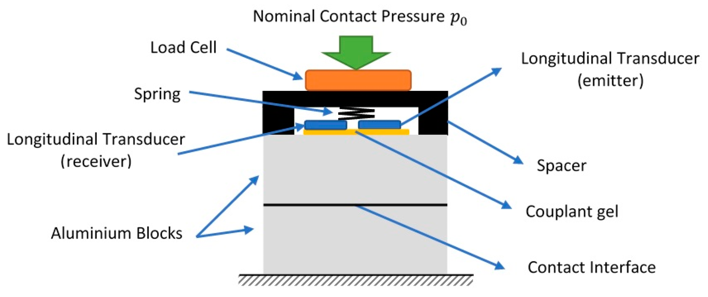
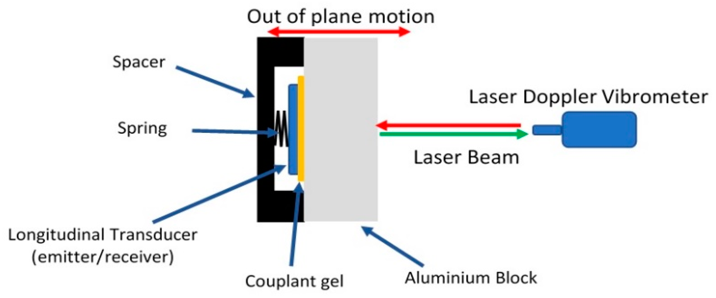
3.1. Loading Apparatus and Specimens

Figure 4 illustrates the experimental apparatus designed for capturing reflected pulses from the interface. Two cylindrical aluminium 6082 T6 blocks, of diameter 39 mm and thickness 32 mm, were loaded together creating a dry contact interface. The load was applied using with a hydraulic material testing machine and measured using a load cell. A spacer was used to protect the sensor location as shown in the figure.

The two specimen contact faces were polished with silicon carbide papers to P2500 grit size and lapped. The arithmetic mean deviation $R_a$, root mean square $R_q$ and mean roughness depth $R_z$ were measured according to ISO 4287 with an optical roughness measurement device (Alicona SL) as shown in

Table 1. Roughness measured before loading/unloading and after 10 loading/unloading cycles.

Process	${\mathit{R}}_{\mathit{a}} \left(\mathsf{\mu }\mathbf{m}\right)$	${\mathit{R}}_{\mathit{q}} \left(\mathsf{\mu }\mathbf{m}\right)$	${\mathit{R}}_{\mathit{z}} \left(\mathsf{\mu }\mathbf{m}\right)$
Before loading/unloading	0.446	0.577	3.092
After 10 loading/unloading cycles	0.404	0.522	2.745

.

Whilst the mean contact pressure is well below the yield stress of the materials, the asperity contacts are at much higher pressure [18] and so experience plastic flow. The plastic flow is greatest at the first loading and then the contact points conform or build up residual stress so subsequent loading is elastic. To ensure all measurements were recorded for an elastic contact, prior to the capturing, 10 loading/unloading cycles at a nominal contact pressure up to 5.5$\mathrm{MPa}$ (which is beyond the nominal contact pressure decided to compress the contacting surfaces ($5 \mathrm{MPa}$)) were applied. Further deformation of the asperity contacts was then expected to be fully elastic.

3.2. Instrumentation

Two piezoelectric longitudinal transducers ($18 \mathrm{mm}$ diameter) with centre frequencies of $2 \mathrm{MHz}$ and $5 \mathrm{MHz}$ were attached on the upper surface of the top aluminium blocks using a couplant gel. The transducer generated the incident wave and caught the signal reflected from the interface. A $2 \mathrm{MHz}$longitidinal toneburst with 11 cycles at different peak-to-peak excitation voltages of $90 \mathrm{V}$, $140 \mathrm{V}$ or $210\mathrm{V}$ was generated and amplified using a high-power amplifier (RITEC RAM-5000). The power generated at these voltages was sufficiently large to generate higher harmonics in reflected pulses from the interface. In this experiment, higher harmonics were observed when the incident wave had a voltage greater than $60\mathrm{V}$ peak-to-peak. The reflected pulses from the contact interface were captured with the longitudinal transducer with centre frequency $5 \mathrm{MHz}$ and stored using a digital oscilloscope. A reference signal was captured from a solid–air contact to eliminate the inherent effect of the materials and consider only the influence of the interface. A PC running LabView was used to trigger the pulsing and receive the digitized reflection data.

3.3. Signal Processing

Figure 5a shows the first and second reflected pulses from the interface of the solid–air contact (reference). This solid–air reflection acts as a reference. Since almost all the sound energy will be reflected from a solid–air interface, this is equivalent to the incident signal. Figure 5d shows the same pulses from a solid–solid contact at nominal contact pressure $4 \mathrm{MPa}$. In the present analysis, only the first reflected pulse was used as this contains most information from the interface.

This first peak was extracted and a Hanning window function and a zero-pad function were applied to increase the resolution of the signals (Figure 5b,e). It should be noted that the type of window function as well as the length of zero-pad function are dependent on the quality of captured signals. In this study, other window functions, such as Hamming window function and Blackman window function were employed, but showed insignificant difference in the results, so the Hanning window function was adopted throughout.

The time domain signals cannot precisely (in most cases this is impossible) indicate the existence of a super-harmonic (higher harmonics), subharmonic, or a mix of both. Therefore, a Fast Fourier Transform was employed to convert the time domain reflected signal to the frequency domain as shown in Figure 5c,f. These peaks are clearly visible corresponding to the fundamental frequency, as well as both, and even and odd (second) harmonics.

Since Figure 5c shows solid–air contact, the source of the higher order harmonics in this case cannot be due to the interfacial contact. This nonlinearity might be generated by the bulk material, bonding nonlinearity (transducers to the specimen), the transducers themselves, or in the amplifier circuitry [29,33,44]. A test to see whether the interface (in the solid-solid case) is a source of harmonics is to increase the nominal contact pressure; this causes a reduction in the amplitude of higher harmonics indicating that the interface is also the source of nonlinearity generated in the reflected signals. To eliminate all sources of nonlinearity apart from those generated by the contact [45,46], Equation (38) is reformulated as:

$$\gamma =\left|\frac{A_2}{A_1^2}-\frac{A_{2 ref}}{A_{1 ref}^2}\right|=\frac{K_2}{\rho c\omega \sqrt{1+{\left(K_1/\rho c\omega \right)}^2}}$$

(40)

where $A_{1 ref}$ and $A_{2 ref}$ are amplitudes of fundamental frequency and second order harmonic from a solid-air contact, respectively. In this way all nonlinearities not associated with the interface are subtracted out.

The amplitude of the fundamental frequency of the reflected pulse in solid–solid contact (Figure 5f) was divided by the amplitude of the corresponding harmonic from the reference solid-air contact (Figure 5c) to derive the reflection coefficient $R$ (Equation (36)). For the second order nonlinear parameter $\gamma$, the amplitude of the fundamental frequency was divided by the square of the amplitude of the second harmonic (Equation (40)).

3.4. Voltage to Meter Conversion

Reflected and transmitted signals received by the transducer from the interface are in units of voltage, therefore, the second order nonlinear parameter for the reflected ultrasound from the interface $\gamma$ is in ${\mathrm{V}}^{-1}$. To compute the nonlinear stiffness $K_2$, the nonlinear parameter for the reflected ultrasound amplitude from the interface $\gamma$ must be in units of meters. A method for determining the amplitude (in meters) from the piezo voltage was required. A Laser Doppler vibrometer (Polytec with laser sensor head OFV 354 and the vibrometer controller OFV 2500) was employed, as shown in Figure 6. A laser beam was incident on the free surface of the aluminium block with a transducer connected to the back face. While the transducer generated longitudinal waves in the aluminium block at different excitation voltages from $70 \mathrm{V}$ to $350 \mathrm{V}$ at center frequency $2 \mathrm{MHz}$, the laser beam was reflected from the free surface and captured by the laser sensor head. The captured laser beam returns velocity information. A numerical integral with respect to time results in the displacement of the surface in meters. The same signal processing procedure as explained in Section 3.3 was used to measure the displacement of the surface at different piezo voltages and hence incident amplitudes.

Figure 7 presents the linear variation of amplitude of the reflected signal from the interface in voltage unit against the displacement of solid–air contact in meter. The slope of the curve $\delta \left(\mathrm{V}/\mathrm{m}\right)$ gives voltage to meter conversion [47]:

$$\gamma \left({\mathrm{m}}^{-1}\right)=\delta \left(\frac{\mathrm{V}}{\mathrm{m}}\right)\gamma \left({\mathrm{V}}^{-1}\right)$$

(41)

4. Results and Discussion

Figure 8a shows the reflection coefficient $R$ for incident waves of excitations $90 \mathrm{V}$, $140 \mathrm{V}$ and $210 \mathrm{V}$ as a function of the nominal contact pressure, determined from the amplitude of the first order reflection from the solid interface divided by that from the solid-air interface according to Equation (36). They were measured after 10 loading/unloading cycles to remove any asperity plasticity effects. It can be seen that the reflection coefficient decreases with increasing the nominal contact pressure due to increase in the real contact area.

The data of Figure 8a was used to determine the first order linear interfacial stiffness $K_1$ using Equation (37) (Figure 8b). Higher pressures cause a stiffer interface. As expected, the reflection coefficient and linear stiffness determined at any voltage is identical. The amplitude of the ultrasonic wave does not change the linear stiffness component.

A best fit curve to the linear interfacial stiffness shown in Figure 8b is a fourth-order polynomial expression [22]:

$$K_1\left(p_0\right)={\displaystyle \sum }_{n=0}^4{a}_n{p}_0{}^n$$

(42)

where $a_n$ is a constant coefficient. This coefficient will depend on factors such as surface topography and elastoplastic deformation of the asperities in contact.

The nominal contact pressure $p_0$ can be expressed in terms of the relative surface approach $Y$ of the contacting surfaces. To do this, the linear interfacial stiffness $K_1$ (Equation (42)) was substituted into Equation (27) creating a first order nonlinear homogeneous differential equation:

$$\frac{dp}{dY}+K_1\left(p_0\right)=0 , p\left(0\right)=0$$

(43)

The initial condition indicates that in the absence of elastic wave (ultrasound), there is zero relative surface approach. The homotopy perturbation method (HPM) was employed to solve Equation (43) with respect to relative surface approach:

$$p_0\left(Y\right)={\displaystyle \sum }_{n=0}^2{b}_n{Y}^n$$

(44)

where $b_n$ is a constant coefficient. This coefficient, as with $a_n$, will also depend on the surface asperity and material properties. A numerical differential equation (ode45 function in MATLAB [48]) of the data in Figure 8b according to Equation (43) was used to determine the nominal contact pressure-relative surface approach relationship, as shown in Figure 8c.

The shape of the nonlinear nominal contact pressure-relative surface approach curve demonstrates the stiffening behaviour of the interfacial spring under increasing contact pressure. In other words, increasing the nominal contact pressure leads to a reduction in the gap, more solid contact, and hence a stiffer interface. In the absence of an elastic wave, the relative surface approach was zero ($Y=0)$ under nominal contact pressure $p_0=0 \mathrm{MPa}$ (nominal contact pressure generated by the weight of upper body is negligible). The negative sign of the relative surface approach $Y$ indicates the reduction of the interface separation (greater deflection in the asperities). The gradient of the curve increases with increase in nominal contact pressure demonstrating stiffer interfacial contact.

Figure 9a shows the second order nonlinear parameter $\gamma$ at excitations $90\mathrm{V}$, $140\mathrm{V}$, and $210\mathrm{V}$ as a function of the nominal contact pressure. This nonlinear parameter is determined from the amplitude of the second harmonic divided by the square of the first harmonic (Equation (40)). To evaluate the second order nonlinear stiffness $K_2$, the experimental results of the second order nonlinear parameter $\gamma$ were substituted into Equation (39) (Figure 9b).

It is seen from Figure 9b that the second order nonlinear stiffness increases as the nominal contact pressure increases up to 2.5 MPa. However, beyond this value the nonlinearity decreases, so the nonlinear stiffness decreases. The comparison shows that $K_2$ is independent of the amplitude of the incident wave. A best fit curve to the second order nonlinear interfacial stiffness $K_2$ shown in Figure 9b is a fourth-order polynomial expression [22]:

$$K_2\left(p_0\right)={\displaystyle \sum }_{n=0}^4{c}_n{p}_0{}^n$$

(45)

where $c_n$ is a constant coefficient. This coefficient depends on some factors such as surface topography and elastoplastic deformation of the asperities in contact. However, further studies are required. As before, the nominal contact pressure $p_0$ is expressed in terms of the relative surface approach $Y$ of the contacting surfaces. To do this, the nonlinear interfacial stiffness $K_2$ (Equation (45)) was substituted into Equation (28) creating a second order nonlinear homogeneous differential equation:

$$\frac{1}{2}\frac{d^{2}p}{d{Y}^2}-K_2\left(p_0\right)=0 , \frac{dp}{dY}=0 , p\left(0\right)=0$$

(46)

The initial conditions indicate that in the absence of an elastic wave (ultrasound), there is zero relative surface approach and linear interfacial stiffness. The homotopy perturbation method (HPM) was again employed to solve Equation (46) with respect to relative surface approach. A numerical differential equation (ode45 function in MATLAB [48]) of the data in Figure 9b according to Equation (46) was used to determine the nominal contact pressure–relative surface approach relationship, as shown in Figure 9c. The result was the same as Equation (44).

The comparison between the pressure–relative surface approach derived from linear and nonlinear interfacial stiffness is presented in Figure 10. Figure 10a shows the pressure-relative surface approach derived from the present experimental data. Figure 10b is included for comparison, and shows the pressure–relative surface derived from the experimental data from [22]. It should be noted that the experiment presented in [22] was through transmission while the current paper considered reflected signal. Both approaches yield a similar relationship.

It is seen that the pressure–approach relationship derived from the linear stiffness $K_1$ and second order nonlinear stiffness $K_2$are very similar for all excitation voltage cases. As expected, the pressure–approach response should not depend on whether it was determined from either linear or nonlinear stiffness measured data. This gives confidence in the robustness of the measurement method and the analysis approach. The interfacial spring can be modelled with a stiffness described by a Taylor expansion with first and second order components (Equation (26)). Further, an experimental measurement of either one of these components, using ultrasonic reflection, is sufficient to deduce the other and hence characterise the spring stiffness.

5. Conclusions

In this work, the stiffness of a rough surface contact has been expressed in terms of a linear and second order nonlinear stiffness. Both these interfacial stiffness components were determined from the refection of a high-power ultrasonic wave. The high-power wave causes a non-linear response of the interface and generates higher order harmonics. The first order linear stiffness was deduced from the reflection of the fundamental frequency wave; whilst the second order nonlinear stiffness was deduced from the second harmonic frequency reflection. A fourth-order polynomial expression for the linear and nonlinear interfacial stiffness as a function of nominal contact pressure were defined. A first order nonlinear homogeneous differential equation of linear stiffness and a second order nonlinear homogeneous differential equation of the nonlinear stiffness with respect to relative surface approach was used to determine the relationship between the nominal contact pressure and relative surface approach. The results derived from both linear and nonlinear interfacial stiffness were similar. This indicates both linear and nonlinear interfacial stiffness subjected to the same nominal contact pressure can be measured by ultrasound. Further, the Taylor series used to represent the contact pressure–relative surface approach relationship can accurately represent the interface behaviour.

References

1. Drinkwater, B.W.; Dwyer-Joyce, R.S.; Cawley, P. A study of the interaction between ultrasound and a partially contacting solid—Solid interface. Proc. R. Soc. A Math. Phys. Eng. Sci. 1996, 452, 2613–2628. [Google Scholar]
2. Thomas, T.R.; Sayles, R.S. Stiffness of Machine Tool Joints: A Random-Process Approach. J. Eng. Ind. 1977, 99, 250–256. [Google Scholar] [CrossRef]
3. Mindlin, R.D. Compliance of Elastic Bodies in Contact. J. Appl. Mech. 1949, 16, 259–268. [Google Scholar] [CrossRef]
4. Greenwood, J.A.; Williamson, J.B.P. Contact of nominally flat surfaces. Proc. R. Soc. Lond. Ser. A Math. Phys. Sci. 1966, 295, 300–319. [Google Scholar]
5. A Onions, R.; Archard, J.F. The contact of surfaces having a random structure. J. Phys. D Appl. Phys. 1973, 6, 289–304. [Google Scholar] [CrossRef]
6. Whitehouse, D.J.; Archard, J.F. The properties of random surfaces of significance in their contact. Proc. R. Soc. Lond. Ser. A Math. Phys. Sci. 1970, 316, 97–121. [Google Scholar] [CrossRef] [Green Version]
7. Bush, A.; Gibson, R.; Thomas, T. The elastic contact of a rough surface. Wear 1975, 35, 87–111. [Google Scholar] [CrossRef]
8. Campana, C.; Persson, B.; Müser, M.H. Transverse and normal interfacial stiffness of solids with randomly rough surfaces. J. Phys. Condens. Matter 2011, 23, 085001. [Google Scholar] [CrossRef] [Green Version]
9. Kartal, M.E.; Mulvihill, D.M.; Nowell, D.; Hills, D.A. Determination of the Frictional Properties of Titanium and Nickel Alloys Using the Digital Image Correlation Method. Exp. Mech. 2011, 51, 359–371. [Google Scholar] [CrossRef]
10. De Crevoisier, J.; Swiergiel, N.; Champaney, L.; Hild, F. Identification of In Situ Frictional Properties of Bolted Assemblies with Digital Image Correlation. Exp. Mech. 2012, 52, 561–572. [Google Scholar] [CrossRef]
11. Mulvihill, D.M.; Brunskill, H.; Kartal, M.E.; Dwyer-Joyce, R.S.; Nowell, D. A Comparison of Contact Stiffness Measurements Obtained by the Digital Image Correlation and Ultrasound Techniques. Exp. Mech. 2013, 53, 1245–1263. [Google Scholar] [CrossRef] [Green Version]
12. Straffelini, G. Surfaces in Contact. In Materials with Internal Structure; Springer: Cham, Switzerland, 2015; Volume 20, pp. 1–20. [Google Scholar] [CrossRef]
13. Chikate, P.; Basu, S. Contact stiffness of machine tool joints. Tribol. Int. 1975, 8, 9–14. [Google Scholar] [CrossRef]
14. Handzel-Powierza, Z.; Klimczak, T.; Polijaniuk, A. On the experimental verification of the Greenwood-Williamson model for the contact of rough surfaces. Wear 1992, 154, 115–124. [Google Scholar] [CrossRef]
15. Królikowski, J.; Szczepek, J. Prediction of contact parameters using ultrasonic method. Wear 1991, 148, 181–195. [Google Scholar] [CrossRef]
16. Sherif, H.; Kossa, S. Relationship between normal and tangential contact stiffness of nominally flat surfaces. Wear 1991, 151, 49–62. [Google Scholar] [CrossRef]
17. Sun, Y.; Xiao, H.; Xu, J. Investigation into the interfacial stiffness ratio of stationary contacts between rough surfaces using an equivalent thin layer. Int. J. Mech. Sci. 2019, 163, 105147. [Google Scholar] [CrossRef]
18. Dwyer-Joyce, R.S.; Drinkwater, B.W.; Quinn, A.M. The Use of Ultrasound in the Investigation of Rough Surface Interfaces. J. Tribol. 2000, 123, 8–16. [Google Scholar] [CrossRef]
19. Tattersall, H.G. The ultrasonic pulse-echo technique as applied to adhesion testing. J. Phys. D Appl. Phys. 1973, 6, 819. [Google Scholar] [CrossRef]
20. Baik, J.-M.; Thompson, R.B. Ultrasonic scattering from imperfect interfaces: A quasi-static model. J. Nondestruct. Eval. 1984, 4, 177–196. [Google Scholar] [CrossRef]
21. Dwyer-Joyce, R.S. The Application of Ultrasonic NDT Techniques in Tribology. Proc. Inst. Mech. Eng. Part J J. Eng. Tribol. 2005, 219, 347–366. [Google Scholar] [CrossRef] [Green Version]
22. Biwa, S.; Hiraiwa, S.; Matsumoto, E. Experimental and theoretical study of harmonic generation at contacting interface. Ultrasonics 2006, 44, 1319–1322. [Google Scholar] [CrossRef] [PubMed]
23. Biwa, S.; Suzuki, A.; Ohno, N. Evaluation of interface wave velocity, reflection coefficients and interfacial stiff-nesses of contacting surfaces. Ultrasonics 2005, 43, 495–502. [Google Scholar] [CrossRef]
24. Kendall, K.; Tabor, D. An ultrasonic study of the area of contact between stationary and sliding surfaces. Proc. R. Soc. Lond. Ser. A Math. Phys. Sci. 1971, 323, 321–340. [Google Scholar]
25. Gonzalez-Valadez, M.; Baltazar, A.; Dwyer-Joyce, R.S. Study of interfacial stiffness ratio of a rough surface in contact using a spring model. Wear 2010, 268, 373–379. [Google Scholar] [CrossRef] [Green Version]
26. Biwa, S.; Hiraiwa, S.; Matsumoto, E. Pressure-Dependent Stiffnesses and Nonlinear Ultrasonic Response of Contacting Surfaces. J. Solid Mech. Mater. Eng. 2009, 3, 10–21. [Google Scholar] [CrossRef]
27. Baltazar, A.; Rokhlin, S.I.; Pecorari, C. On the relationship between ultrasonic and micromechanical properties of contacting rough surfaces. J. Mech. Phys. Solids. 2002, 50, 1397–1416. [Google Scholar] [CrossRef]
28. Krolikowski, J.; Szczepek, J.; Witczak, Z. Ultrasonic investigation of contact between solids under high hydrostatic pressure. Ultrason. 1989, 27, 45–49. [Google Scholar] [CrossRef]
29. Yan, D.; Drinkwater, B.W.; Neild, S.A. Measurement of the ultrasonic nonlinearity of kissing bonds in adhesive joints. NDT E Int. 2009, 42, 459–466. [Google Scholar] [CrossRef]
30. Rokhlin, S.I.; Wang, Y.J. Analysis of boundary conditions for elastic wave interaction with an interface between two solids. J. Acoust. Soc. Am. 1991, 89, 503–515. [Google Scholar] [CrossRef]
31. Du, F.; Hong, J.; Xu, Y. An acoustic model for stiffness measurement of tribological interface using ultrasound. Tribol. Int. 2014, 73, 70–77. [Google Scholar] [CrossRef]
32. Xiao, H.; Sun, Y. An improved virtual material based acoustic model for contact stiffness measurement of rough interface using ultrasound technique. Int. J. Solids Struct. 2018, 155, 240–247. [Google Scholar] [CrossRef]
33. Breazeale, M.A.; Thompson, D.O. Finite-amplitude ultrasonic waves in aluminum. Appl. Phys. Lett. 1963, 3, 77–78. [Google Scholar] [CrossRef]
34. Zabusky, N.J. Interpretation of the “stabilization distance” as evidence of weak shock formation in low-loss longitudinal nonlinear wave propagation experiments. Phys. Chem. Solids 1965, 26, 955–958. [Google Scholar] [CrossRef]
35. Buck, O.; Morris, W.L.; Richardson, J.M. Acoustic harmonic generation at unbonded interfaces and fatigue cracks. Appl. Phys. Lett. 1978, 33, 371–373. [Google Scholar] [CrossRef]
36. Severin, F.M.; Solodov, I.Y. Experimental Observation of Acoustic Demodulation in Reflection from a Solid-Solid Interface. Phys. Acoust. 1989, 35, 447–448. [Google Scholar]
37. Ko, S.L.; Severin, F.M.; Solodov, I.Y. Experimental Observation of the Influence of Contact Nonlinearity on the Re-flection of Bulk Acoustic Waves and the Propagation of Surface Acoustic Waves. Sov. Phys. Acoust. 1991, 37, 610–612. [Google Scholar]
38. Richardson, J.M. Harmonic generation at an unbonded interface—I. Planar interface between semi-infinite elastic media. Int. J. Eng. Sci. 1979, 17, 73–85. [Google Scholar] [CrossRef]
39. Biwa, S.; Nakajima, S.; Ohno, N. On the Acoustic Nonlinearity of Solid-Solid Contact with Pressure-Dependent Interface Stiffness. J. Appl. Mech. 2004, 71, 508–515. [Google Scholar] [CrossRef]
40. Hirose, S. 2-D scattering by a crack with contact-boundary conditions. Wave Motion 1994, 19, 37–49. [Google Scholar] [CrossRef]
41. Jhang, K. Nonlinear Ultrasonic Techniques for Nondestructive Assessment of Micro Damage in Material: A review. Int. J. Precis. 2009, 10, 123–135. [Google Scholar]
42. Budynas, R.G.; Nisbett, J.K.; Tangchaichit, K. Shigley’s Mechanical Engineering Design, 10th ed.; McGraw-Hill Education: New York, NY, USA, 2011. [Google Scholar]
43. He, J.-H. Homotopy perturbation method: A new nonlinear analytical technique. Appl. Math. Comput. 2003, 135, 73–79. [Google Scholar] [CrossRef]
44. Hurley, D.C.; Fortunko, C.M. Determination of the nonlinear ultrasonic parameter using a Michelson interferom-eter Determination of the nonlinear ultrasonic parameter β using a Michelson interferometer. Meas. Sci. Technol. 1997, 8, 634–642. [Google Scholar] [CrossRef]
45. Blanloeuil, P.; Croxford, A.J.; Meziane, A. Numerical and experimental study of the nonlinear interaction between a shear wave and a frictional interface. J. Acoust. Soc. Am. 2014, 135, 1709–1716. [Google Scholar] [CrossRef]
46. Li, X.; Dwyer-Joyce, R.S. Measuring friction at an interface using ultrasonic response. Proc. R. Soc. A Math. Phys. Eng. Sci. 2020, 476, 20200283. [Google Scholar] [CrossRef] [PubMed]
47. Biwa, S.; Yamaji, S.; Matsumoto, E. Quantitative Evaluation of Harmonic Generation at Contacting Interface. AIP Conf. Proc. 2008, 1022, 505–508. [Google Scholar] [CrossRef]
48. Shampine, L.F.; Reichelt, M.W. The MATLAB ODE Suite. SIAM J. Sci. Comput. 1997, 18, 1–22. [Google Scholar] [CrossRef] [Green Version]
Figure 1. Schematic diagram of the asperity junctions and ultrasonic wave propagation through the media [1,39]: (a) aluminium blocks and aspeiry contact in the absence of normal load; (b) origin and direction of the positive propagation axis; (c) contacting surfaces in the absence of elastic wave under static equilibrium contact; (d) relative surface approach and surface separation due to propagating elastic wave.
Applsci 11 05720 g001
Figure 2. Schematic diagram of higher harmonic generation at an incomplete interface [41]: (a) rough surface interface modelled as array of gaps; (b) incidents ultrasonic wave interacts with the interface; (c) approaching surfaces; (d) being apart surfaces.
Applsci 11 05720 g002
Figure 3. A theoretical approach for Contact Acoustic Nonlinearity (CAN) mechanics at incident wave amplitude 20 nm: (a) comparison between incident wave and gap separation h variation with time; (b) comparison between reflected wave from solid-air contact (reference signal) and solid-solid contact at 2 MPa; (c) effect of nominal contact pressure on reflected wave from solid-solid contact at 2 MPa and 3 MPa; (d) frequency spectrum comparison between incident wave, solid-solid contact at 2 MPa and 3 MPa.
Applsci 11 05720 g003
Figure 4. Schematic diagram of ultrasound reflection measuring apparatus.
Applsci 11 05720 g004
Figure 5. Signal processing of the reflected pulses from interface using a 140 V excitation with incident frequency 2 MHz: (ac) solid-air contact (reference signal); (df) solid-solid contact at nominal contact pressure 4   MPa ; (a,d) time domain of generated, first and second reflected pulses; (b,e) Hanning window and zero pad result of the first reflected pulse; (c,f) Fast Fourier Transform (FFT) results of the first reflected pulse.
Applsci 11 05720 g005
Figure 6. Schematic diagram of voltage to meter conversion apparatus.
Applsci 11 05720 g006
Figure 7. Voltage to meter conversion at ultrasonic incident amplitudes 70 V, 90 V, 140 V, 210 V, 280 V and 350 V.
Applsci 11 05720 g007
Figure 8. The influence of nominal contact pressure p 0 : (a) reflection coefficient; (b) linear interfacial stiffness; (c) pressure-relative surface approach derived from the linear interfacial stiffness at incidents amplitude excitations of 90   V , 140   V and 210   V .
Applsci 11 05720 g008
Figure 9. The influence of nominal contact pressure p 0 : (a) second order nonlinear parameter for the reflected ultrasound from the interface γ ; (b) nonlinear interfacial stiffness; (c) pressure-relative surface approach derived from the nonlinear interfacial stiffness at incidents amplitude excitations of 90   V , 140   V and 210   V .
Applsci 11 05720 g009
Figure 10. Pressure-relative surface approach derived from linear and nonlinear interfacial stiffness: (a) experimental data of the current study at incidents amplitude excitations of 90   V , 140   V and 210   V ; (b) experimental data from [22] at incidents amplitude excitations of 374   V .
Applsci 11 05720 g010