An Effective Adaptive Combination Strategy for Distributed Learning Network

Abstract

In this paper, we develop a modified adaptive combination strategy for the distributed estimation problem over diffusion networks. We still consider the online adaptive combiners estimation problem from the perspective of minimum variance unbiased estimation. In contrast with the classic adaptive combination strategy which exploits orthogonal projection technology, we formulate a non-constrained mean-square deviation (MSD) cost function by introducing Lagrange multipliers. Based on the Karush–Kuhn–Tucker (KKT) conditions, we derive the fixed-point iteration scheme of adaptive combiners. Illustrative simulations validate the improved transient and steady-state performance of the diffusion least-mean-square LMS algorithm incorporated with the proposed adaptive combination strategy.

1. Introduction

It is generally beneficial to exploit diffusion strategies for distributed parameter estimation issues over adaptive networks [1,2,3,4,5,6]. Specifically, the diffusion least-mean-square (LMS)-based methods have already been used in many contexts, such as biological behavior modeling [7,8], distributed detection [9], distributed localization [10] and target tracking and escaping from predators [11], where scalability, robustness, and low power consumption are the desirable features [1]. For the diffusion strategy, each node of the network is allowed to receive the intermediate estimates from its neighboring nodes to improve the accuracy of its local estimate. Such cooperation enables each node to leverage the spatial diversity of noise profile over the entire network. From this point of view, the performance of distributed diffusion methods can be further enhanced by using suitable combination weights (combiners).

There have been several static combination rules [1,12], e.g., Metropolis rule, Laplacian rule, Uniform rule and Relative-degree rule. However, these static combiners are designed based solely on the topology of network, so they would generally be unadjustable to adapt to the spatial variation of signal and noise statistics. To address this problem, many studies resort to the adaptive combination (AC) strategies [12,13,14,15,16,17,18], most of which are developed for the adapt-then-combine (ATC) diffusion LMS algorithm [1].

Based on the minimum variance unbiased estimation (MVUE), the classic AC strategy [12] outperforms existing static combiners when applying onto the diffusion LMS algorithms. An optimal adaptive combination scheme is derived by estimating the variances of the measurement noises adaptively [13]. Simulation results validate the superior steady-state performance of the diffusion LMS algorithm regarding the optimal combiners in [13], as compared to previous static and adaptive combiners. Based on the adaptive combination rule in [13], an optimal combination rule regarding the channel distortion is also proposed [16]. To achieve both the accelerated convergence rate and good steady-state network performance, the combination switching mechanisms [14,15] are proposed, i.e., static combination scheme in the converging stage and AC scheme when approaching the steady state.

In addition, a decoupled adapt-then-combine (D-ATC) algorithm is proposed, for, the least-squares (LS)-based AC scheme is developed [17,18], which could achieve rather approximate performance as the ATC algorithm with the classic AC in homogeneous networks.

Motivation and Contribution

As mentioned above, the classic AC strategy is derived based on MVUE, which is validated to be a feasible criterion [12]. In fact, one of the key techniques in the classic AC strategy [12] is orthogonal projection which is exploited to guarantee the combiners adding up to 1. However, the orthogonal projection technique actually limits the update direction of combiners at each iteration, which can be relaxed to further improve the performance of diffusion LMS algorithm further ahead in Section 3.2.

In this paper, we still formulate the online adaptive combiners estimation of the ATC algorithm from the perspective of MVUE. Instead of directly exploiting the orthogonal projection technology in [12], we present a non-constrained mean-square deviation (MSD) cost function based on Lagrange multipliers. According to the fixed-point iteration methodology and KKT necessary conditions, we develop an effective adaptive combination strategy, which solely relies on the previous instantaneous intermediate weight estimates without resorting to the knowledge of measurement data and noises. The proposed AC strategy can be seen as the modified and extended version of the classic AC in [12]. Simulations validate the superior performance of the diffusion LMS algorithm when using the proposed AC strategy.

Notation: $\mathbb{R}$ and $\mathbb{C}$ denote the fields of real and complex numbers, respectively. Scalars are denoted by lower-case letters, and vectors and matrices respectively by lower- and upper-case boldface letters. The transpose and conjugate transpose are denoted by ${(·)}^{\mathrm{T}}$ and ${(·)}^{\mathrm{H}}$, respectively. $E\{·\}$ represents expectation. $\Re (·)$ means the real part. $\mathrm{col}\{·\}$ stands for the vector obtained by stacking its arguments on top of one another. $\mathrm{diag}\{·\}$ generates a diagonal matrix using the given diagonal arguments. ${[·]}_i$ stands for the ith element of a vector. The $min\{·\}$ denotes the minimum element of a vector. We define the eigenvalue set of the square matrix $\mathit{F}$ as $\left\{\lambda \right(\mathit{F}\left)\right\}$, with ${\lambda }_{max}\left(\mathit{F}\right)$ denoting the maximum eigenvalue. The spectral radius of the square matrix $\mathit{F}$ is denoted by $\varrho \left(\mathit{F}\right)\triangleq max\left\{\right|\lambda \left(\mathit{F}\right)\left|\right\}$.

2. The ATC Diffusion LMS Algorithm

2.1. Model Assumption

Consider a network containing N nodes, which are used to estimate an M-dimensional unknown parameter ${\mathit{w}}_o\in {\mathbb{C}}^M$ collectively. ${\mathcal{N}}_k$ denotes the set of neighbors of node k, including k itself. The cardinality of ${\mathcal{N}}_k$ is $n_k$. For each node k, at the time instant t, the regressor ${\mathit{u}}_k\left(t\right)\in {\mathbb{C}}^M$ and the measurement signal $d_k\left(t\right)\in \mathbb{C}$ are available. The signal model is given by

$$d_k\left(t\right)\triangleq {\mathit{w}}_o^{\mathrm{H}}{\mathit{u}}_k\left(t\right)+v_k\left(t\right),$$

(1)

where $v_k\left(t\right)$ denotes the additive zero-mean white Gaussian measurement noise at node k, with variance ${\sigma }_{v,k}^2$. For any k and t, $v_k\left(t\right)$ is independent from ${\mathit{u}}_k\left(t\right)$, and for all $k\ne l$ or $i\ne j$, $v_k\left(i\right)$ is independent from $v_l\left(j\right)$.

2.2. ATC Algorithm

The main target of distributed estimation algorithm is to generate an estimate ${\mathit{w}}_k\left(t\right)$ of ${\mathit{w}}_o$ at each node k and time t in a distributed manner. For the diffusion strategy, generally, each node k executes a local adaptation step to obtain an intermediate estimate ${\mathit{\psi }}_k\left(t\right)$, then all the nodes share their intermediate estimates to their neighbors, and finally, each node k linearly combines all the intermediate estimates received from its neighbors under some combination weights. The detailed steps of ATC diffusion LMS algorithm are

$$\begin{array}{cc}\hfill {\mathit{\psi }}_k\left(t\right)& ={\mathit{w}}_k(t-1)+{\mu }_k{\mathit{u}}_k\left(t\right){\mathit{e}}_k^{*}\left(t\right),\hfill \end{array}$$

(2)

$$\begin{array}{cc}\hfill {\mathit{w}}_k\left(t\right)& ={\sum }_{l\in {\mathcal{N}}_k}{a}_{l,k}{\mathit{\psi }}_l\left(t\right),\hfill \end{array}$$

(3)

where ${\mathit{e}}_k\left(t\right)\triangleq d_k\left(t\right)-{\mathit{w}}_k^{\mathrm{H}}(t-1){\mathit{u}}_k\left(t\right)$ is the prior estimate error and ${\mu }_k>0$ is the step size for $k\in \{1,2,\dots ,N\}$. The combiner $a_{l,k}$ is the weight of intermediate estimation from node l during the combination step of node k. Moreover, the non-negative combination matrix $\mathit{A}=\left[a_{l,k}\right]$ satisfies [1,12]

$$a_{l,k}\ge 0\mathrm{if}l\in {\mathcal{N}}_k,a_{l,k}=0\mathrm{if}l\notin {\mathcal{N}}_k,{\mathit{a}}_k^{\mathrm{T}}\mathbf{1}=1,$$

(4)

with ${\mathit{a}}_k$ denoting the kth column of $\mathit{A}$. Notice that $\mathit{A}$ is left-stochastic since the entries of each column are non-negative and sum to 1 [19,20].

3. Adaptive Combination Scheme

3.1. Minimum Variance Unbiased Estimation

Consider the signal model and the ATC diffusion LMS algorithm in Section 2. Assume that for each node $k\in \{1,\dots ,N\}$, the intermediate estimate ${\mathit{\psi }}_k\left(t\right)$ in the diffusion LMS algorithm satisfies

$$E\left\{{\mathit{\psi }}_k\left(t\right)\right\}={\mathit{w}}_o,\mathrm{for}\mathrm{all}k\in \{1,\dots ,N\},$$

(5)

We define

$$\begin{array}{cc}\hfill & \mathbf{\Psi }\left(t\right)\triangleq [{\mathit{\psi }}_1\left(t\right),\dots ,{\mathit{\psi }}_N\left(t\right)],k=1,\cdots ,N.\hfill \end{array}$$

Following [12], we have the minimum variance unbiased estimation problem for each $k\in \{1,\dots ,N\}$,

$$\begin{array}{cccc}\hfill & \hfill & \hfill \underset{{\mathit{a}}_k\in {\mathbb{R}}^N}{min}& {\mathit{a}}_k^T\Re \left({\mathit{Q}}_{\mathbf{\Psi }}\right){\mathit{a}}_k\hfill \\ \hfill & \hfill & \hfill \mathrm{st}.& {\mathbf{1}}_N^T{\mathit{a}}_k=1;a_{l,k}=0,\mathrm{for}\mathrm{all}l\notin {\mathcal{N}}_k,\hfill \end{array}$$

(6)

where ${\mathit{Q}}_{\mathbf{\Psi }}\triangleq E\left\{{(\mathbf{\Psi }\left(t\right)-E\left\{\mathbf{\Psi }\left(t\right)\right\})}^{\mathrm{H}}(\mathbf{\Psi }\left(t\right)-E\left\{\mathbf{\Psi }\left(t\right)\right\})\right\}$ and ${\mathbf{1}}_N$ denotes the $N\times 1$ vector with unit entries. Applying the convex combination strategy $\mathrm{for}\mathrm{all}k\in \{1,\dots ,N\}$, we also require $a_{l,k}⩾0$.

3.2. Fixed-Point Iteration Solution

First, we introduce a transform matrix ${\mathit{P}}_k$, defined as ${\mathit{P}}_k\triangleq {\left[l\mathrm{th}\mathrm{column}\mathrm{of}{\mathit{I}}_N\right]}_{l\in {\mathcal{N}}_k}$. Then, ${\mathit{a}}_k$ in (6) can be expressed by ${\mathit{a}}_k={\mathit{P}}_k{\mathit{b}}_k$, with ${\mathit{b}}_k\in {\mathbb{R}}^{n_k}$. Therefore, the minimization problem (6) can be transformed into

$$\begin{array}{cccc}\hfill & \hfill & \hfill \underset{{\mathit{b}}_k}{min}& J\left({\mathit{b}}_k\right)\triangleq {\mathit{b}}_k^T\Re \left({\mathit{Q}}_{{\mathbf{\Psi }}_k}\right){\mathit{b}}_k\hfill \\ \hfill & \hfill & \hfill \mathrm{st}.& {\mathbf{1}}_{n_k}^T{\mathit{b}}_k=1;b_{k,i}\ge 0,\mathrm{for}i=1,\dots ,n_k,\hfill \end{array}$$

(7)

where ${\mathit{Q}}_{{\mathbf{\Psi }}_k}\triangleq {\mathit{P}}_k^T{\mathit{Q}}_{\mathbf{\Psi }}{\mathit{P}}_k=E\left\{{({\mathbf{\Psi }}_k\left(t\right)-E\left\{{\mathbf{\Psi }}_k\left(t\right)\right\})}^{\mathrm{H}}({\mathbf{\Psi }}_k\left(t\right)-E\left\{{\mathbf{\Psi }}_k\left(t\right)\right\})\right\}$ with ${\mathbf{\Psi }}_k\left(t\right)\triangleq \mathbf{\Psi }\left(t\right){\mathit{P}}_k$, and $b_{k,i}$ is the ith element of vector ${\mathit{b}}_k$. By introducing the Lagrange multipliers $\alpha$ and $\mathbf{\omega }$, we obtain the cost function

$$\mathcal{L}({\mathit{b}}_k,\mathbf{\omega },\alpha )\triangleq J\left({\mathit{b}}_k\right)-{\mathbf{\omega }}^T{\mathit{b}}_k+\alpha ({\mathbf{1}}_{n_k}^T{\mathit{b}}_k-1).$$

(8)

Taking the gradient of (8) with respect to ${\mathit{b}}_k$ yields

$$\begin{array}{cc}\hfill {\nabla }_{{\mathit{b}}_k}\mathcal{L}({\mathit{b}}_k,\mathbf{\omega },\alpha )& ={\nabla }_{{\mathit{b}}_k}J\left({\mathit{b}}_k\right)-\mathbf{\omega }+{\mathbf{1}}_{n_k}\alpha \hfill \\ \hfill & =\Re \left({\mathit{Q}}_{{\mathbf{\Psi }}_k}\right){\mathit{b}}_k-\mathbf{\omega }+{\mathbf{1}}_{n_k}\alpha .\hfill \end{array}$$

(9)

According to the Karush–Kuhn–Tucker (KKT) condition [21], the optimal value of the tuple (${\mathit{b}}_k,\mathbf{\omega },\alpha$) should obey

$$\left\{\begin{array}{c}\Re \left({\mathit{Q}}_{{\mathbf{\Psi }}_k}\right){\mathit{b}}_k-\mathbf{\omega }+{\mathbf{1}}_{n_k}\alpha =0\hfill \\ {\left[\mathbf{\omega }\right]}_i{b}_{k,i}=0\hfill \end{array}\right..$$

(10)

or equivalently,

$${[\Re \left({\mathit{Q}}_{{\mathbf{\Psi }}_k}\right){\mathit{b}}_k+{\mathbf{1}}_{n_k}\alpha ]}_i{b}_{k,i}=0.$$

(11)

We introduce a positive definite diagonal matrix ${\mathit{D}}_k(t-1)$, whose ith diagonal element is an arbitrary positive function with respect to ${\mathit{b}}_k(t-1)$, denoted as $f_i\left({\mathit{b}}_k(t-1)\right)$. Obviously, ${\mathit{D}}_k(t-1)\left(-{\nabla }_{{\mathit{b}}_k}\mathcal{L}({\mathit{b}}_k,\mathbf{\omega },\alpha )\right)$ is still the descent direction of the cost function (8) [21]. Therefore, we have the adaptive solution of problem (7) through the fixed-point iteration method

$$\begin{array}{cc}\hfill b_{k,i}\left(t\right)=& b_{k,i}(t-1)-{\eta }_{k,i}\left(t\right)f_i\left({\mathit{b}}_k(t-1)\right)b_{k,i}(t-1)\hfill \\ \hfill & {[\Re \left({\mathit{Q}}_{{\mathbf{\Psi }}_k}\right){\mathit{b}}_k(t-1)+{\mathbf{1}}_{n_k}\alpha ]}_i,\hfill \end{array}$$

(12)

where $b_{k,i}\left(t\right)$ is the estimate of $b_{k,i}$ at time instant t and ${\eta }_{k,i}$ is the learning factor of $b_{k,i}\left(t\right)$.

To simplify the problem, we choose the same learning factor ${\eta }_{k,i}$ for all i at any time t. Hence, we can rewrite (12) as a vector,

$$\begin{array}{cc}\hfill {\mathit{b}}_k\left(t\right)=& {\mathit{b}}_k(t-1)-{\eta }_k\left(t\right){\mathbf{\Gamma }}_k(t-1)[\Re \left({\mathit{Q}}_{{\mathbf{\Psi }}_k}\right){\mathit{b}}_k(t-1)+{\mathbf{1}}_{n_k}\alpha ].\hfill \end{array}$$

(13)

where ${\mathbf{\Gamma }}_k(t-1)\triangleq \mathrm{diag}\left\{{\mathit{D}}_k(t-1){\mathit{b}}_k(t-1)\right\}$.

Applying the constraint ${\mathbf{1}}_{n_k}^T{\mathit{b}}_k\left(t\right)=1$ and pre-multiplying both sides of (13) by ${\mathbf{1}}_{n_k}^T$ yields the Lagrange multiplier $\alpha$

$$\alpha =\frac{{\mathbf{1}}_{n_k}^T({\mathit{b}}_k(t-1)-{\eta }_k\left(t\right){\mathbf{\Gamma }}_k(t-1)\Re \left({\mathit{Q}}_{{\mathbf{\Psi }}_k}\right){\mathit{b}}_k(t-1))-1}{{\eta }_k\left(t\right){\mathbf{1}}_{n_k}^T{\mathbf{\Gamma }}_k(t-1){\mathbf{1}}_{n_k}}.$$

(14)

Substituting $\alpha$ into (13), and using the constraint ${\mathbf{1}}_{n_k}^T{\mathit{b}}_k(t-1)=1$ again, we can obtain the update of combiners ${\mathit{b}}_k\left(t\right)$,

$$\begin{array}{cc}\hfill {\mathit{b}}_k\left(t\right)& ={\mathit{b}}_k(t-1)-{\eta }_k\left(t\right){\mathit{G}}_k(t-1){\mathbf{\Gamma }}_k(t-1)\Re \left({\mathit{Q}}_{{\mathbf{\Psi }}_k}\right){\mathit{b}}_k(t-1).\hfill \end{array}$$

(15)

where ${\mathit{G}}_k(t-1)\triangleq {\mathit{I}}_{n_k}-\frac{{\mathit{D}}_k(t-1){\mathit{b}}_k(t-1){\mathbf{1}}_{n_k}^T}{{\mathbf{1}}_{n_k}^T{\mathit{D}}_k(t-1){\mathit{b}}_k(t-1)}$ with ${\mathit{I}}_{n_k}$ denoting the $n_k\times n_k$ identity matrix.

The adaptive combiners (15) can be updated by two incremental steps

$$\begin{array}{cc}\hfill {\mathit{g}}_k\left(t\right)& ={\mathbf{\zeta }}_k(t-1)\Re \left({\mathit{Q}}_{{\mathbf{\Psi }}_k}\right){\mathit{b}}_k(t-1)\hfill \end{array}$$

(16)

$$\begin{array}{cc}\hfill {\mathit{b}}_k\left(t\right)& ={\mathit{b}}_k(t-1)-{\eta }_k\left(t\right){\mathit{g}}_k\left(t\right)\hfill \end{array}$$

(17)

where

$$\begin{array}{c}\hfill {\mathbf{\zeta }}_k(t-1)={\mathit{G}}_k(t-1){\mathbf{\Gamma }}_k(t-1).\end{array}$$

(18)

Then, we can obtain the combiner ${\mathit{a}}_k\left(t\right)$

$$\begin{array}{cc}\hfill {\mathit{a}}_k\left(t\right)& ={\mathit{P}}_k{\mathit{b}}_k\left(t\right)\hfill \end{array}$$

(19)

which can be used in (3) to update the local weight estimate adaptively. We also define the adaptive combination matrix $\mathit{A}\left(t\right)\in {\mathbb{R}}^{N\times N}$ where ${\mathit{a}}_k\left(t\right)$ is the kth column vector of it.

Please note that $-{\mathit{g}}_k\left(t\right)$ in (16) can be seen as the product of ${\mathbf{\zeta }}_k(t-1)$ and the gradient ${\nabla }_{{\mathit{b}}_k}J\left({\mathit{b}}_k(t-1)\right)=\Re \left({\mathit{Q}}_{{\mathbf{\Psi }}_k}\right){\mathit{b}}_k(t-1)$, which means ${\mathbf{\zeta }}_k(t-1)$ can be seen an auxiliary matrix to adjust the update direction ${\nabla }_{{\mathit{b}}_k}J\left({\mathit{b}}_k(t-1)\right)$. On the one hand, note that ${\mathit{G}}_k(t-1)$ in (18) is a projection matrix [22], which enables the update direction $-{\mathit{g}}_k\left(t\right)$ orthogonal to the vector ${\mathbf{1}}_{n_k}$, i.e., ${\mathbf{1}}_{n_k}^T{\mathit{g}}_k\left(t\right)=0$. Then we have ${\mathbf{1}}_{n_k}^T{\mathit{b}}_k\left(t\right)={\mathbf{1}}_{n_k}^T{\mathit{b}}_k(t-1)=\cdots ={\mathbf{1}}_{n_k}^T{\mathit{b}}_k\left(0\right)=1$ if the initial combiners satisfy ${\mathbf{1}}_{n_k}^T{\mathit{b}}_k\left(0\right)=1$. On the other hand, since as a whole, ${\mathbf{\zeta }}_k(t-1)$ is a positive semi-definite symmetric matrix, the update direction $-{\mathit{g}}_k\left(t\right)$ is still the descent direction of the cost function (7) [21]. Instead of using the positive semi-definite symmetric matrix ${\mathbf{\zeta }}_k(t-1)={\mathit{G}}_k(t-1){\mathbf{\Gamma }}_k(t-1)$, the classic AC [12] consider ${\mathbf{\zeta }}_k(t-1)$ being replaced by the orthogonal projection matrix characterized by ${\mathbf{1}}_{n_k}$, i.e., ${\mathit{I}}_{n_k}-\frac{{\mathbf{1}}_{n_k}{\mathbf{1}}_{n_k}^T}{n_k}$, which actually limits the update direction of the adaptive combiners to be lie in the hyperplane spanned by ${\mathbf{1}}_{n_k}$ and ${\nabla }_{{\mathit{b}}_k}J\left({\mathit{b}}_k(t-1)\right)$. In fact, we find that (16) and (17) could reduce to the classic AC [12] when ${\mathit{D}}_k\left(t\right)=\mathrm{diag}{\left\{{\mathit{b}}_k\left(t\right)\right\}}^{-1}$.

We now consider optimizing the learning factor ${\eta }_k\left(t\right)$. Substituting (16) and (17) into (7) yields a cost function regarding the learning factor ${\eta }_k\left(t\right)$,

$$\begin{array}{cc}\hfill h\left({\eta }_k\left(t\right)\right)& ={\mathit{g}}_k^T\left(t\right)\Re \left({\mathit{Q}}_{{\mathbf{\Psi }}_k}\right){\mathit{g}}_k\left(t\right){\eta }_k^2\left(t\right)\hfill \\ \hfill & -2{\mathit{g}}_k^T\left(t\right)\Re \left({\mathit{Q}}_{{\mathbf{\Psi }}_k}\right){\mathit{b}}_k(t-1){\eta }_k\left(t\right)\hfill \\ \hfill & +{\mathit{b}}_k^T(t-1)\Re \left({\mathit{Q}}_{{\mathbf{\Psi }}_k}\right){\mathit{b}}_k(t-1).\hfill \end{array}$$

(20)

Obviously, $h\left({\eta }_k\left(t\right)\right)$ is a quadratic (convex) function with respect to ${\eta }_k\left(t\right)$. Thus, its minimum value can be readily obtained if and only if

$$\begin{array}{cc}\hfill {\eta }_k^o\left(t\right)& ={\displaystyle \frac{{\mathit{g}}_k^T\left(t\right)\Re \left({\mathit{Q}}_{{\mathbf{\Psi }}_k}\right){\mathit{b}}_k(t-1)}{{\mathit{g}}_k^T\left(t\right)\Re \left({\mathit{Q}}_{{\mathbf{\Psi }}_k}\right){\mathit{g}}_k\left(t\right)}}\hfill \\ \hfill & ={\displaystyle \frac{{\mathit{b}}_k^T(t-1)\Re \left({\mathit{Q}}_{{\mathbf{\Psi }}_k}\right){\mathbf{\zeta }}_k(t-1)\Re \left({\mathit{Q}}_{{\mathbf{\Psi }}_k}\right){\mathit{b}}_k(t-1)}{{\mathit{g}}_k^T\left(t\right)\Re \left({\mathit{Q}}_{{\mathbf{\Psi }}_k}\right){\mathit{g}}_k\left(t\right)}}.\hfill \end{array}$$

(21)

Note that the optimal learning factor ${\eta }_k^o\left(t\right)$ is non-negative since ${\mathbf{\zeta }}_k(t-1)$ is a positive semi-definite matrix.

To guarantee that the combiners are non-negative, we set the upper bound of ${\eta }_k\left(t\right)$ as [12],

$$\begin{array}{c}\hfill {\eta }_k^{max}\left(t\right)={\displaystyle \frac{min\left({\mathit{b}}_k\left(t\right)\right)}{\parallel {\mathit{g}}_k{\left(t\right)\parallel }_{\infty }+\epsilon }},\end{array}$$

(22)

where $\epsilon >0$ is a small constant. Please note that ${\parallel ·\parallel }_{\infty }$ represents the maximum norm. Thus, we choose the learning factor in (17) at time instant t,

$$\begin{array}{c}\hfill {\eta }_k\left(t\right)=min\{{\eta }_k^{max}\left(t\right),{\eta }_k^o\left(t\right)\}.\end{array}$$

(23)

Please note that the ${\mathit{Q}}_{{\mathbf{\Psi }}_k}$ is usually unavailable in practical applications. As what done in [12], ${\mathit{Q}}_{{\mathbf{\Psi }}_k}$ can be replaced by its approximation

$$\begin{array}{c}\hfill {\widehat{\mathit{Q}}}_{{\mathbf{\Psi }}_k}\left(t\right)\approx \frac{1}{2}\Delta {\mathbf{\Psi }}_k^H\left(t\right)\Delta {\mathbf{\Psi }}_k\left(t\right).\end{array}$$

(24)

where $\Delta {\mathbf{\Psi }}_k\left(t\right)={\mathbf{\Psi }}_k\left(t\right)-{\mathbf{\Psi }}_k(t-1)$. To make it smoother, we consider a forgetting factor $\lambda$. Then, the iterative expression of ${\widehat{\mathit{Q}}}_{{\mathbf{\Psi }}_k}$ can be written as

$$\begin{array}{c}\hfill {\widehat{\mathit{Q}}}_{{\mathbf{\Psi }}_k}\left(t\right)=\lambda {\widehat{\mathit{Q}}}_{{\mathbf{\Psi }}_k}(t-1)+\frac{1}{2}\Delta {\mathbf{\Psi }}_k^H\left(t\right)\Delta {\mathbf{\Psi }}_k\left(t\right).\end{array}$$

(25)

In practical applications, we use ${\widehat{\mathit{Q}}}_{{\mathbf{\Psi }}_k}\left(t\right)$ in (25) to replace the aforementioned statistical quantity ${\mathit{Q}}_{{\mathbf{\Psi }}_k}$ for each node k at time instant t.

Finally, the implementation of the ATC algorithm with the proposed AC strategy is summarized in Algorithm 1.

Algorithm 1 ATC with the proposed AC strategy

For each node k, set ${\mathit{\psi }}_k\left(0\right)={\mathit{w}}_k\left(0\right)={\mathbf{0}}_M$ and choose ${\mathit{b}}_k\left(0\right)\in {\mathbb{R}}^{n_k}$ so that ${\mathbf{1}}_{n_k}^T{\mathit{b}}_k\left(0\right)=1$. Given a small positive constant $\epsilon$ and step size ${\mu }_k$, at each time instant $t>0$, compute at each node k: 1. Update the intermediate weight estimate ${\mathit{\psi }}_k\left(t\right)$ through (2). 2. Update combiner ${\mathit{a}}_k\left(t\right)$ consecutively through (25), (16), (23), (17) and (19). 3. Update the local weight estimate ${\mathit{w}}_k\left(t\right)$ through (3).

4. Mean Convergence

We now analyze the mean convergence of the diffusion LMS algorithm with the proposed adaptive combiners.

We now introduce the following independence assumptions:

Assumption 1

(Independence). All regressors ${\mathit{u}}_k\left(t\right)$ are spatially and temporally independent ([1], Assumption 1).

Assumption 2.

The combination matrix $\mathit{A}\left(t\right)$ is independent of all regressors ${\mathit{u}}_k\left(t\right)$ and all local weight estimates ${\mathit{w}}_k(t-1)$ at time $t-1$ ([12], Assumption 4.3).

Theorem 1.

Under Assumptions 1 and 2, a sufficient condition to guarantee the convergence of the diffusion LMS algorithm is given by,

$$\begin{array}{c}\hfill 0<{\mu }_k<{\displaystyle \frac{2}{\varrho \left(\mathit{R}\right)}},\end{array}$$

(26)

where $\varrho \left(\mathit{R}\right)$ denotes the spectrum radius of the matrix $\mathit{R}$.

The proof is referred to Appendix A. Please note that the sufficient condition (26) is consistent with ([1], Equation (37)) and ([12], Equation (25))

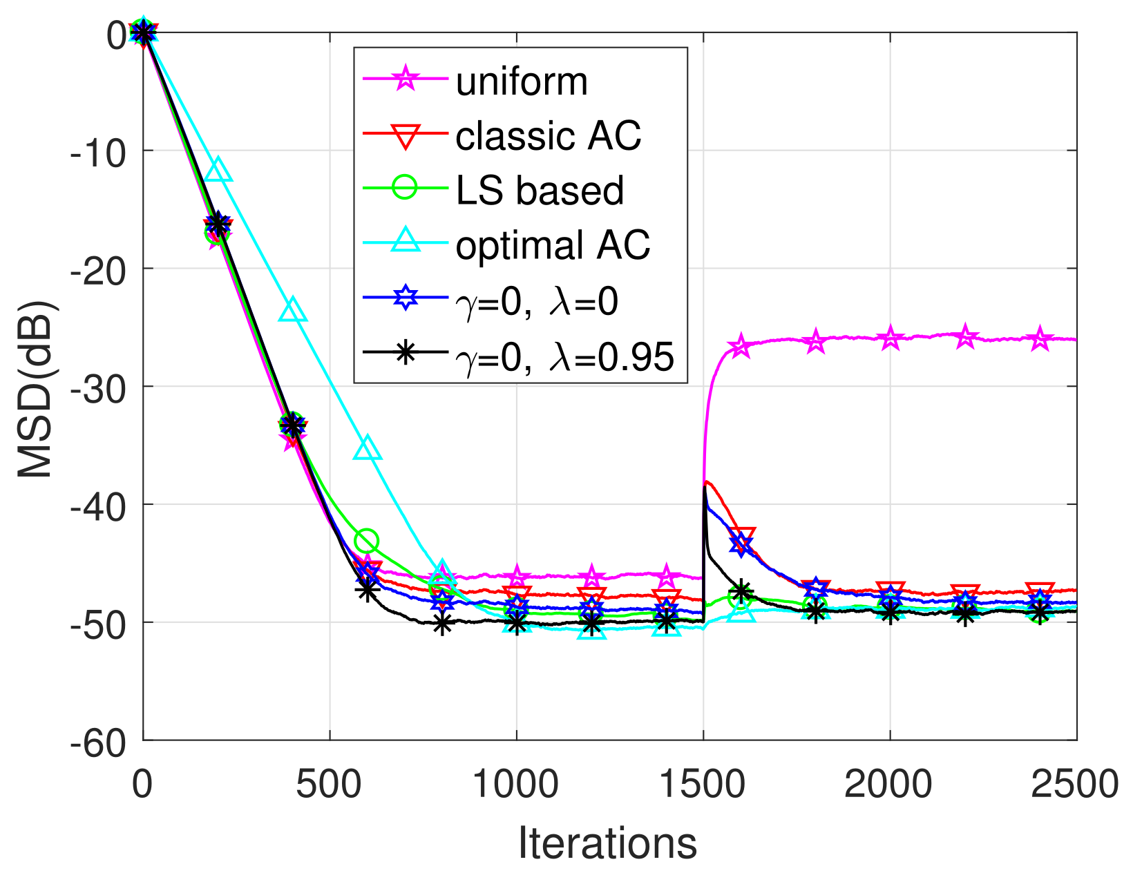
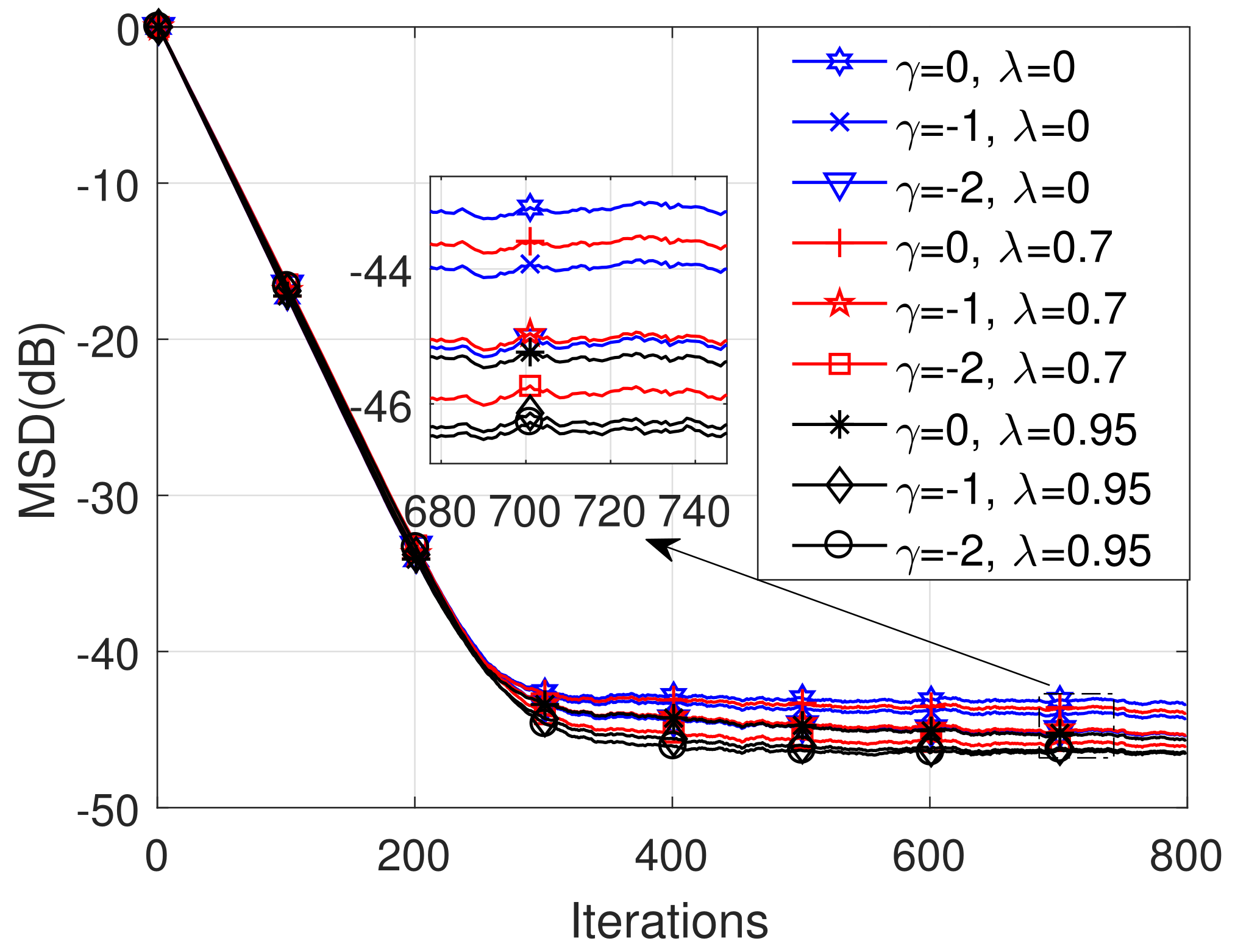
5. Simulation Results

We evaluate herein the MSD of the proposed algorithm. Without loss of generality, the unknown weight vector ${\mathit{w}}_o$ is set to be ${\mathbf{1}}_M/M$ with $M=5$. The initial weight vector estimations are ${\mathit{w}}_k\left(0\right)={\mathbf{0}}_M$ for each node k. The constant $\epsilon$ used in (22) is set to be $0.5\times {10}^{-4}$ and the forgetting factor $\lambda =0$ or $\lambda =0.95$. We consider ${\mathit{D}}_k\left(t\right)=\mathrm{diag}{\left\{{\mathit{b}}_k\left(t\right)\right\}}^{\gamma }$ in terms of the proposed AC, where $\gamma$ can be 0, −1 or −2.

We use the empirical MSDs as the performance metrics. Both the transient and steady-state empirical network MSDs hereinafter are obtained by averaging $\mathcal{L}=500$ independent trials over all nodes of the network,

$$\begin{array}{cc}\hfill \mathcal{MSD}\left(t\right)& \triangleq {\displaystyle \frac{1}{\mathcal{L}N}}{\sum }_{k=1}^N{\sum }_{\ell =1}^{\mathcal{L}}{\parallel {\tilde{\mathit{w}}}_k^{(\ell )}\left(t\right)\parallel }_2^2,\hfill \end{array}$$

(27)

$$\begin{array}{cc}\hfill \mathcal{MSD}& \triangleq {\displaystyle \frac{1}{\mathcal{L}N}}{\sum }_{k=1}^N{\sum }_{\ell =1}^{\mathcal{L}}{\parallel {\tilde{\mathit{w}}}_k^{(\ell )}(\infty )\parallel }_2^2,\hfill \end{array}$$

(28)

where ${\tilde{\mathit{w}}}_k^{(\ell )}\left(t\right)\triangleq {\mathit{w}}_{\mathrm{o}}-{\mathit{w}}_k^{(\ell )}\left(t\right)$ with ${\mathit{w}}_k^{(\ell )}\left(t\right)$ denoting the transient weight estimate of the ℓth trial and $\parallel {\tilde{\mathit{w}}}_k^{(\ell )}{(\infty )\parallel }_2^2$ is obtained by averaging $\parallel {\tilde{\mathit{w}}}_k^{(\ell )}{\left(t\right)\parallel }_2^2$ of 100 iterations after convergence.

Example 1.

We consider the same topology of the network with $N=15$ nodes as ([12], Figure 5) ([17], Figure 6a), illustrated in Figure 1a. The measurement noise is real Gaussian white noise with its variance ${\sigma }_{v,k}^2$ at each node k presented in Figure 1b. According to the mean convergence condition, we set the step size to ${\mu }_k=0.01$ for each node k. We herein consider $\gamma =0$. Each regressor ${\mathit{u}}_k\left(t\right)$ at each node k is real Gaussian white noise sequence with their covariance matrices ${\mathit{R}}_{u,k}={\sigma }_{u,k}^2{\mathit{I}}_M$ with ${\sigma }_{u,k}^2=1$ for all k. The noise power of node $5,12,13$ at the 1500th iteration suddenly goes up to 5.

As demonstrated in Figure 2, the proposed AC strategy outperforms the classic AC [12] and the uniform combination [1] in terms of superior steady-state performance and similar convergence rates, and outperforms LS-based AC [17] and the optimal AC [13] in terms of accelerated convergence rate. We also observe that the forgetting factor can further enhance the performance of the proposed AC. After the sudden change of the noise power of some nodes, the proposed AC exhibits rather high reconvergence rate and good steady-state performance.

Example 2.

The initial measurement noise variance ${\sigma }_{v,k}^2$ at each node k is presented in Figure 1b. In this simulation, we compare the proposed AC scheme with the uniform combination and the classic AC in terms of the steady-state MSD at different noise variances $\tau {\sigma }_{v,k}^2$ at each node k. The other simulation conditions are same as Example 1. The steady-state MSDs with respect to the noise variances are illustrated in

Table 1. The steady-state MSD with respect to the variation of the noise power.

	Combiners	Uniform	Classic AC	$\mathit{\lambda }=0$	$\mathit{\lambda }=0.95$
Noise $\mathit{\tau }$
$\tau =0.5$		−49.0	−50.2	−51.2	−53.0
$\tau =1$		−46.0	−48.0	−49.1	−50.0
$\tau =1.5$		−44.3	−46.6	−47.7	−48.3
$\tau =2$		−43.3	−45.9	−46.9	−47.1
$\tau =2.5$		−42.1	−45.1	−46.1	−46.1
$\tau =3$		−41.2	−44.3	−45.2	−45.3
$\tau =3.5$		−40.6	−43.7	−44.4	−44.4
$\tau =4$		−40.2	−43.5	−44.1	−44.0
$\tau =4.5$		−39.6	−42.9	−43.5	−43.3
$\tau =5$		−39.2	−42.7	−43.3	−43.2

.

The fairness of this experiment is endorsed by the relatively approximate convergence behavior of the transient MSD curves plotted in Figure 3. As shown in Table 1, with the noise variances increasing, the ATC algorithm incorporated with the proposed AC exhibits superior performance compared to the ATC algorithm with the uniform combination or the classic AC strategy. Additionally, we can also find that the performance gain brought by the forgetting factor is limited when the noise variances increase to some certain limit.

Example 3.

We now consider target tracking model ([17], Equation (52)), namely

$$\begin{array}{cc}\hfill {\mathit{w}}_o\left(t\right)& ={\mathit{w}}_o+\mathbf{\theta }\left(t\right)\hfill \end{array}$$

(29)

$$\begin{array}{cc}\hfill \mathbf{\theta }\left(t\right)& =0.99\mathbf{\theta }(t-1)+\mathbf{\xi }\left(t\right)\hfill \end{array}$$

(30)

where $\mathbf{\xi }\left(t\right)$ is a sequence of independent identically distributed perturbations with zero mean and covariance matrix Ξ, independent of the input regressors and measurement noise at every iteration. We herein consider $\mathbf{\xi }\left(t\right)$ is Gaussian white with $\mathbf{\Xi }={\sigma }_{\xi }^2{\mathbf{I}}_M$ and ${\sigma }_{\xi }^2=1\times {10}^{-7}$, i.e., the unknown weight vector is varying slowly. The other simulation conditions are same as Example 1.

As illustrated in Figure 4, similar to Example 1, the proposed AC strategy outperforms the uniform combination rule, the classic AC and LS-based AC in terms of superior steady-state performance, and outperforms the optimal AC in terms of accelerated convergence rate, under tracking scenarios. We could also observe that the forgetting factor can further enhance the performance of the proposed AC in the tracking scenario.

Example 4.

We now consider the impact of the factors λ and γ in the performance of the proposed AC strategy. Without loos of generality, we consider the step sizes ${\mu }_k=0.02$ for each node k. The simulation result is shown in Figure 5.

It can be seen from Figure 5 that with specific $\gamma$, the larger $\lambda$ brings the higher performance gain for the proposed AC. We could also observe that choosing $\gamma =-2$ brings better steady-state performance than the other two choices, especially for small forgetting factor $\lambda$. In particular, as compared to Example 1, for the two scenarios $\gamma =0,\lambda =0$ and $\gamma =0,\lambda =0.95$, we find that larger step sizes in this example lead to accelerated convergence rate at the cost of degraded steady-state performance.

Example 5.

We consider the sparse network with $N=15$ nodes with its topology same as ([12], Figure 8), depicted in Figure 6a. The measurement noise is real Gaussian white noise with its variance ${\sigma }_{v,k}^2$ at each node presented in Figure 6c. We consider the heterogenous network with the step sizes ${\mu }_k=0.004$ for orange shaded nodes and ${\mu }_n=0.02$ for the rest. Each regressor ${\mathit{u}}_k\left(t\right)$ at each node k is real Gaussian white noise sequence with their covariance matrices ${\mathit{R}}_{u,k}={\sigma }_{u,k}^2{\mathbf{I}}_M$ with ${\sigma }_{u,k}^2$ presented in Figure 6b for all k.

As illustrated in Figure 7, for the sparse network, the proposed AC scheme outperforms the classic AC and LS-based AC in terms of superior steady-state performance while keeping rather approximate convergence rate. It also outperforms the optimal AC scheme in terms of the accelerated convergence rate. Moreover, the introduction of forgetting factor can further enhance the performance of the proposed AC scheme.

6. Conclusions

In this paper, we present a modified adaptive combination strategy for the distributed estimation problem over diffusion networks to improve robustness against the spatial variation of signal and noise statistics over the network. Considering the Karush–Kuhn–Tucker conditions and fixed-point iteration methodology, we derive an effective adaptive combination strategy for the ATC diffusion LMS algorithm. We also invoke the forgetting factor and optimize the learning factor to further enhance the performance of the proposed adaptive combination strategy. Illustrative simulations validate the improved performance of the diffusion LMS algorithm with the proposed adaptive combination strategy.

References

1. Cattivelli, F.S.; Sayed, A.H. Diffusion LMS Strategies for Distributed Estimation. IEEE Trans. Signal Process. 2010, 58, 1035–1048. [Google Scholar] [CrossRef]
2. Lee, H.S.; Kim, S.E.; Lee, J.W.; Song, W.J. A Variable Step-Size Diffusion LMS Algorithm for Distributed Estimation. IEEE Trans. Signal Process. 2015, 63, 1808–1820. [Google Scholar] [CrossRef]
3. Ahn, D.C.; Lee, J.W.; Shin, S.J.; Song, W.J. A new robust variable weighting coefficients diffusion LMS algorithm. Signal Process. 2017, 131, 300–306. [Google Scholar] [CrossRef]
4. Huang, W.; Li, L.; Li, Q. Diffusion Robust Variable Step-Size LMS Algorithm Over Distributed Networks. IEEE Access 2018, 6, 47511–47520. [Google Scholar] [CrossRef]
5. Ashkezari-Toussi, S.; Sadoghi-Yazdi, H. Robust diffusion LMS over adaptive networks. Signal Process. 2019, 158, 201–209. [Google Scholar] [CrossRef]
6. Nassif, R.; Vlaski, S.; Sayed, A.H. Adaptation and Learning Over Networks Under Subspace Constraints—Part I: Stability Analysis. IEEE Trans. Signal Process. 2020, 68, 1346–1360. [Google Scholar] [CrossRef] [Green Version]
7. Tu, S.Y.; Sayed, A.H. Mobile adaptive networks with self-organization abilities. In Proceedings of the 2010 7th International Symposium on Wireless Communication Systems, York, UK, 19–22 September 2010; pp. 379–383. [Google Scholar] [CrossRef]
8. Cattivelli, F.S.; Sayed, A.H. Modeling Bird Flight Formations Using Diffusion Adaptation. IEEE Trans. Signal Process. 2011, 59, 2038–2051. [Google Scholar] [CrossRef]
9. Cattivelli, F.S.; Sayed, A.H. Distributed detection over adaptive networks using diffusion adaptation. IEEE Trans. Signal Process. 2011, 59, 1917–1932. [Google Scholar] [CrossRef]
10. Chen, J.; Sayed, A.H. Diffusion Adaptation Strategies for Distributed Optimization and Learning Over Networks. IEEE Trans. Signal Process. 2012, 60, 4289–4305. [Google Scholar] [CrossRef] [Green Version]
11. Tu, S.; Sayed, A.H. Mobile Adaptive Networks. IEEE J. Sel. Top. Signal Process. 2011, 5, 649–664. [Google Scholar] [CrossRef]
12. Takahashi, N.; Yamada, I.; Sayed, A.H. Diffusion Least-Mean Squares with adaptive combiners: Formulation and performance analysis. IEEE Trans. Signal Process. 2010, 58, 4795–4810. [Google Scholar] [CrossRef]
13. Tu, S.; Sayed, A.H. Optimal combination rules for adaptation and learning over networks. In Proceedings of the 2011 4th IEEE International Workshop Computational Advances in Multi-Sensor Adaptive Processing, San Juan, Puerto Rico, 13–16 December 2011; pp. 317–320. [Google Scholar] [CrossRef]
14. Yu, C.; Sayed, A.H. A strategy for adjusting combination weights over adaptive networks. In Proceedings of the 2013 IEEE International Conference Acoustic, Speech and Signal Processing, Vancouver, BC, Canada, 26–31 May 2013; pp. 4579–4583. [Google Scholar] [CrossRef]
15. Fernandez-Bes, J.; Arenas-García, J.; Sayed, A.H. Adjustment of combination weights over adaptive diffusion networks. In Proceedings of the 2014 IEEE International Conference Acoustic, Speech and Signal Processing, Florence, Italy, 4–9 May 2014; pp. 6409–6413. [Google Scholar] [CrossRef]
16. Abdolee, R.; Vakilian, V. An Iterative Scheme for Computing Combination Weights in Diffusion Wireless Networks. IEEE Wireless Commun. Lett. 2017, 6, 510–513. [Google Scholar] [CrossRef]
17. Fernandez-Bes, J.; Azpicueta-Ruiz, L.A.; Arenas-García, J. Distributed estimation in diffusion networks using affine least-squares combiners. Dig. Signal Process. 2015, 36, 1–14. [Google Scholar] [CrossRef]
18. Fernandez-Bes, J.; Arenas-García, J.; Silva, M.T.M. Adaptive Diffusion Schemes for Heterogeneous Networks. IEEE Trans. Signal Process. 2017, 65, 5661–5674. [Google Scholar] [CrossRef] [Green Version]
19. Sayed, A.H. Adaptive Networks. Proc. IEEE 2014, 102, 460–497. [Google Scholar] [CrossRef]
20. Zhao, X.; Sayed, A.H. Asynchronous Adaptation and Learning Over Networks-Part I: Modeling and Stability Analysis. IEEE Trans. Signal Process. 2015, 63, 811–826. [Google Scholar] [CrossRef]
21. Chen, J.; Richard, C.; Bermudez, J.C.M. Nonnegative Least-Mean-Square Algorithm. IEEE Trans. Signal Process. 2011, 59, 5225–5235. [Google Scholar] [CrossRef] [Green Version]
22. Behrens, R.T.; Scharf, L.L. Signal processing applications of oblique projection operators. IEEE Trans. Signal Process. 1994, 42, 1413–1424. [Google Scholar] [CrossRef] [Green Version]
23. Kailath, T.; Sayed, A.H.; Hassibi, B. Linear Estimation; Prentice-Hall: Englewood Cliffs, NJ, USA, 2000. [Google Scholar]
24. Sayed, A.H. Fundamentals of Adaptive Filtering; Wiley: New York, NY, USA, 2003. [Google Scholar]
25. Marshall, A.W.; Olkin, I.; Arnold, B.C. Matrix Theory. In Inequalities: Theory of Majorization and Its Applications; Springer: New York, NY, USA, 2011; Chapter 9; pp. 338–347. [Google Scholar] [CrossRef]
Figure 1. Network topology and noise profile: (a) network topology; (b) noise profile.
Applsci 11 05723 g001
Figure 2. The MSD learning curves.
Applsci 11 05723 g002
Figure 3. The MSD learning curves under different noise levels.
Applsci 11 05723 g003
Figure 4. The MSD learning curves under tracking scenarios.
Applsci 11 05723 g004
Figure 5. The MSD learning curves.
Applsci 11 05723 g005
Figure 6. The topology, regressor power and noise profile: (a) network topology; (b) regressor power; (c) noise profile.
Applsci 11 05723 g006
Figure 7. The MSD learning curves for the sparse network.
Applsci 11 05723 g007