Abstract
One of the most important aspects that need to be addressed to increase solar energy penetration is the power ramp-rate control. In weak grids such as the one found in Puerto Rico, it is important to smooth power fluctuations caused by the intermittence of passing clouds. In this work, a novel power ramp-rate control strategy is proposed. Additionally, a comparison with some of the most common power ramp-rate control methods is performed using a proposed model and real solar radiation data from the Coto Laurel photovoltaic power plant located in Ponce, Puerto Rico. The proposed model was validated using one-year real data from Coto Laurel. The power ramp-rate control methods were compared in real-time simulations using the OP5700 from Opal-RT Technologies considering power ramp rate fluctuations, power ramp-rate violations, fluctuations in the state-of-charge, among other indicators. Moreover, the proposed power ramp-rate control strategy, called predictive dynamic smoothing was explained and compared. Results indicate that the predictive dynamic smoothing produced a considerably reduced Levelized Cost of Storage compared to other power ramp-rate control methods and provided a higher lifetime expectancy for lithium batteries.
1. Introduction
Electrical energy in Puerto Rico has been mainly produced using imported fossil fuels. For the fiscal year of 2020, petroleum-based power plants supplied almost half of the total power generation, while coal-based power plants supplied 29%, and renewable energies only supplied 2.5% [1]. The Puerto Rico Electric Power Authority (PREPA) is aimed to increase renewable energy penetration to 40% by 2025, 60% by 2040, and 100% by 2050 [2]. Particularly, solar energy is the renewable resource that has grown the most with an increase in supply from 0.3% in 2015 to 1.4% in 2020 [3]. Additionally, PREPA is aimed to add up 2740 MW and 1440 MW in solar power and batteries, respectively in the following years [4]. Due to the inherent stochastic nature of solar irradiance, factors such as frequency and voltage stability of a converter-dominated power system (CDPS) may be critically affected on cloudy days. To overcome this issue, some local power authorities across the world have imposed solar power plants to include power ramp-rate control (PRRC) methods in their power injection controllers. A maximum power ramp-rate (PRR) of 10% of the contracted power capacity per minute is allowed in Germany, whereas Hawaii, Ireland, and Denmark allow a maximum PRR of 2 MW/min, 30 MW/min, and 100 kW/s respectively [5,6].
The Puerto Rico Energy Bureau (PREB) has developed a regulation on renewable energy development—including its registration and operation—as a strategy for rebuilding and strengthening the electric power system. The Bureau’s purpose is to increase the local renewable energy generation and provide a regulatory framework for the implementation of renewable energy across the island. One of the most important requirements described in the regulation is the Power Purchase and Operation Agreement (PPOA) or electric power contract. The PPOA is a document that establishes an energy contract between two parties (the seller and the buyer). This contract contains mutual obligations between the parts involved in the power sale, that governs the rights and duties of the parties [7]. One of the most important requirements for third-party photovoltaic (PV) power plants stipulated in the PPOA is the Minimum Technical Requirements for the Interconnection of Photovoltaic Installations (MTR). MTRs are mandatory requirements that the third-party seller must meet to help the main grid in case of contingencies. In the MTR, the ramp rate requirement is addressed, which sets the maximum rate of change for the system’s output power. This maximum rate applies for both, increasing and decreasing the output power with a requirement of 10% of the contracted capacity. Additionally, the current MTR requires the third-party systems to be able to deliver 30% of their measured AC capacity for at least 25 min using their storage units [8].
To fulfill PRR requirements and smooth power fluctuations, large-scale solar power plants (LSSPP) rely on the use of energy storage systems (ESS). The state-of-charge (SOC), the output power Pout, and the depth-of-discharge (DoD) of the ESS through a day may vary drastically depending on the PRRC method and the type of battery used. These factors directly impact battery degradation and the levelized cost of storage (LCOS) [9,10,11]. Thus, LSSPP may incur extra costs in ESS depending on the implemented PRRC method. The ramp-saturation (RS) is the simplest PRRC method [12,13]. In this method, the battery absorbs or injects power when the PRR at the point of interconnection (POI) exceeds the requirement. The Simple Moving Average (SMA) and the Exponential Moving Average (EMA) are also two popular methods due to their low computational cost and ease of implementation [14,15,16,17]. However, the RS, MA, and EMA methods require a large ESS storage capacity [13,18,19]. This implies an increase in costs and battery degradation. PRRC methods such as the Enhanced Linear Exponential Smoothing (ELES) [20,21,22,23], the First Order Low-Pass filter (FOLPF) [24,25,26,27], and the second-order LPF (SOLPF) have been proposed to reduce power fluctuations in the ESS [28]. A solution to avoid the use of ESS is the Active Power Curtailment (APC) method [5,29,30,31,32,33,34]. This method moves the power converter away from the maximum power point to reduce the power injection to the main grid. Though, the APC is only valid for ramp-up events. For this purpose, the Forecasted APC (FAPC) method has been proposed in [35,36]. This method determines whether a ramp-down event will occur and reduces the injected power by moving the power reference away from the maximum power point. However, as both APC and FAPC are aimed to avoid the use of ESS, their reliability is highly affected by the accuracy of the forecast.
As each of the aforementioned PRRC methods has its own advantages and disadvantages, it becomes of high interest to study how they affect the operational costs and how they affect the battery degradation in LSSPP. Furthermore, it becomes important to study the performance of each PRRC method in an LSSPP in Puerto Rico, which is characterized to have a special solar radiation behavior and different grid characteristics compared to other territories. Other studies about the impact of PRRC have been made in Puerto Rico [5,37,38]. However, none of them have tested the impact of different PRRC methods nor their impact on battery degradation.
This work is intended to propose a predictive PRRC method and to perform a study comparing the aforementioned PRRC methods applied to a case study in a highly detailed model of the Coto Laurel solar power plant. Coto Laurel is a solar farm in Ponce, a town located on the southern coast of Puerto Rico. The installed capacity is approximately 14 MW DC, distributed in fifteen (15) groups of solar panels, for a total of 55,416 panels. The contracted capacity at the POI is 10 MW. Figure 1 shows the satellite view of the solar farm, each of the fifteen groups is depicted with a white box. Moreover, each group was labeled with a black capital letter to simplify the discussion. The green boxes depict the location of the inverters and their respective transformers, whereas the orange box shows the farm’s battery bank and its respective inverters and transformers to connect to the main grid.

Figure 1.
Coto Laurel Satellite View. Photo from Map Data © 2021 Google.
The model of the Coto Laurel solar power plant was developed, tested, and validated using an OP5700 simulator from OPAL-RT technologies. Furthermore, the proposed predictive PRRC method was compared against others PRRC methods to analyze the effect in the LCOS and the battery degradation.
The rest of this document is organized as follows: In Section 2, a brief overview of the most common PRRC methods is made. Then, in Section 3, the proposed predictive PRRC method is presented. Section 4 presents the methodology for the economic analysis of each of the PRRC methods. Section 5 presents the case study in Coto Laurel, Puerto Rico. Section 6 presents daily and yearly simulation results and a comparative analysis Finally, discussions and highlighting are presented in Section 7.
2. Overview of the Power Ramp-Rate Control Methods
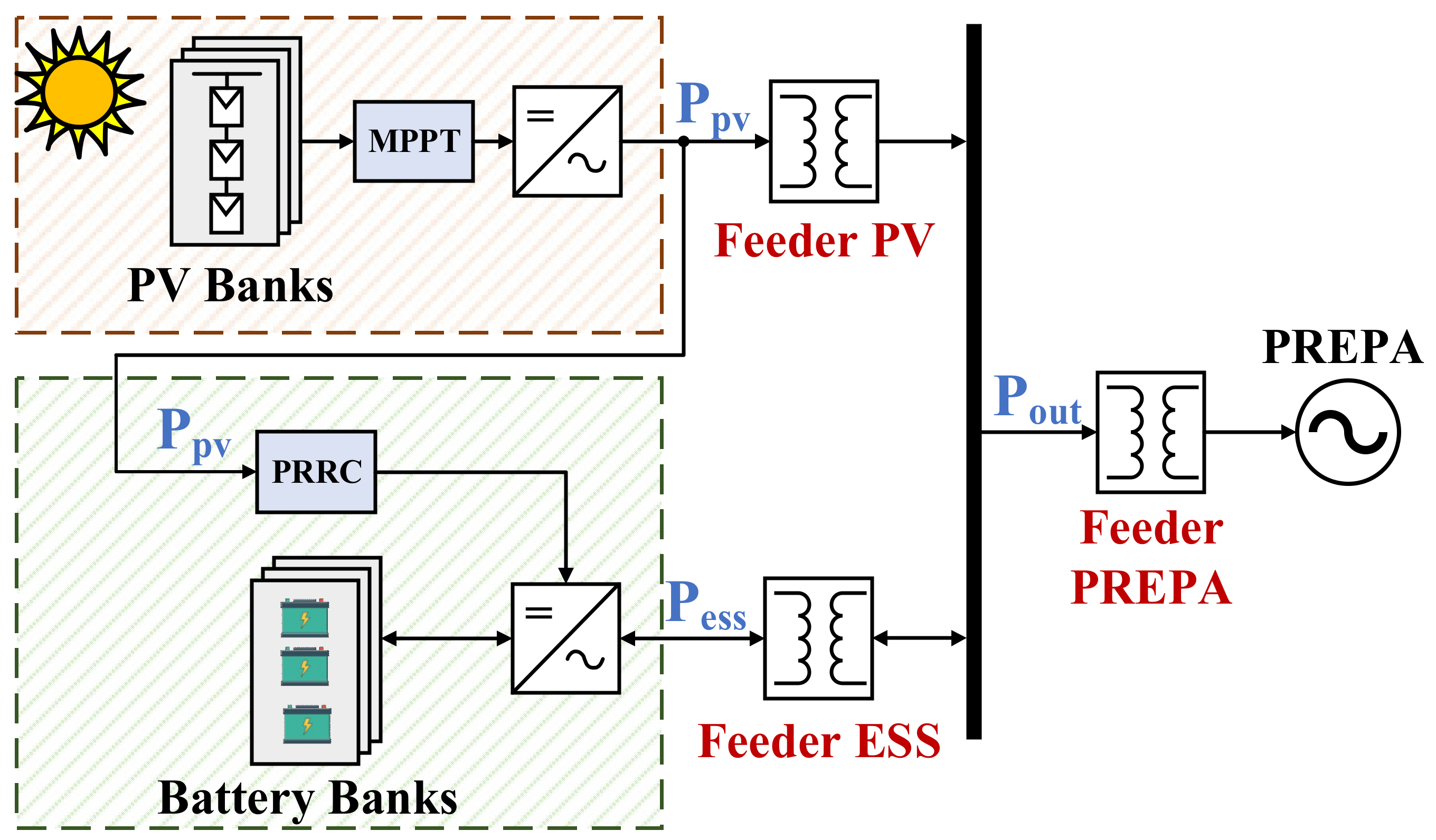
A simplified scheme of an LSSPP with PRRC, similar to Coto Laurel, is shown in Figure 2. The DC voltage of each PV array is transformed to AC using three-phase voltage-source converters (VSC). The output of each converter is connected to PREPA using a central feeder transformer. Similarly, the ESS is composed of a set of battery banks. The voltage of each battery bank is transformed to AC using a VSC. The ESS has its own transformer to inject or absorb power from the AC bus. The PRRC block reads the power in the PV feeder and generates a power reference to the VSC so that the power injected into the main grid fulfills the PRR requirements.
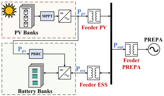
Figure 2.
Basic scheme of an LSSPP with PRRC.
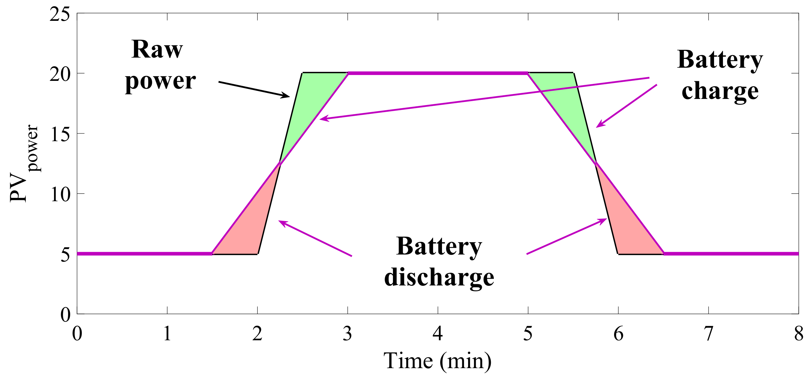
The output power in the ESS feeder can be positive (battery charge) or negative (battery discharge). As seen in Figure 3, when the PRR in the PV violates the requirement, the battery absorbs or injects energy to smooth the output power to the main grid.
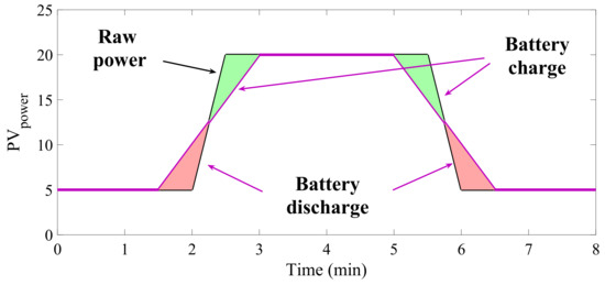
Figure 3.
Battery behavior during PRR events.
Depending on the PRRC method, the battery may achieve a higher or lower DoD, and the SOC at the end of the day may vary as well. These two factors drastically affect the battery degradation and the cost associated with ESS for PRRC.
Following, a brief description of each of the PRRC methods analyzed in this work is presented. To simplify notation, the power injected into the main grid is represented by:
Furthermore, the PRR of the power injected by the PV array at time t = kTs is represented by:
where is the sampling period. Additionally, the maximum allowed PRR at the POI by regulation is defined as .
2.1. Ramp Saturation (RS) Method
The RS is one of the most common and easy-to-implement PRRC methods. This method evaluates the PRR of the PV and absorbs or delivers energy from the ESS to saturate the PRR at the output. The RS method can be expressed as [12,13]:
As decreases, the ESS VSC will require more energy to smooth power transitions at the output. Thus, the DoD of the ESS will increase because the SOC will reach lower values.
2.2. Simple Moving Average (SMA) Method
The SMA method is known for its ease of implementation and because it allows for adjusting PRR fluctuations. The mathematical expression for the SMA method is given by [14,15]:
where W is the window size for calculating the average. For this method, as the window size W becomes larger, the power fluctuations at the output become softer. However, this implies more DoD and more computational cost.
2.3. Exponential Moving Average (EMA) Method
The EMA method is an extension of the SMA. However, this method takes priority on recent samples by using an exponential weighting function as follows [16,17]:
where the exponential smoothing factor is between 0 and 1. As becomes closer to 1, more priority is given to older samples. As this method gives more priority to recent samples, it is more suitable for smoothing power peaks at the output while maintaining the mean value.
2.4. First Order Low-Pass Filter (FOLPF) Method
The FOLPF is used to suppress high frequencies from the input signal with an attenuation factor of −20 dB/dec after the cutoff frequency of the oscillations. In the case of PRRC, the cutoff frequency should be selected to attenuate oscillations in the PV power. Thus, it is important to analyze the worst-case power oscillation that can be observed during the day. The output equation for the FOLPF is given by [24,25,26,27]:
where
and is the inverse z-transform operator. The terms and are the sampling period and the time constant, respectively. As the ratio becomes larger, the bandwidth of the FOLPF increases. It is important to note that, if become larger than 2, the eigenvalues of become located outside the unitary circle and the FOLPF will become unstable. Thus, the desired transient response must be selected in terms of the sampling period.
2.5. Second Order Low-Pass Filter (SOLPF) Method
The SOLPF is similar to the FOLPF. However, the attenuation factor for the SOLPF is −40 db/DB. This implies that the SOLPF is more selective below the cutoff frequency, compared to the FOLPF. This implies that high-frequency fluctuations in the PV power can be more attenuated, which helps to reduce PRR violations. The discrete transfer function for the SOLPF is given by [28]:
where is the natural frequency and is the damping ratio. As the eigenvalue location of is not as explicit as , it is important to analyze them before implementation.
2.6. Enhanced Linear Exponential Smoothing (ELES)
The ELES method performs two complementary exponential smoothing operations. Although this method has high mathematical complexity, it is known to have a better performance compared to the aforementioned methods [19]. The mathematical expression for the ELES is given by [20,21,22,23]:
where and are auxiliary variables for computing the double complementary filter. Constant is the smoothing factor, which is required to be selected between 0 and 1.
3. Proposed Predictive Dynamic Smoothing PRRC Method
The proposed Predictive Dynamic Smoothing (PDS) method uses predicted PV output power values to adjust the PRR considering future power fluctuations. For example, if the prediction indicates that there will be a ramp-down violation, the PDS method will charge the battery prior to that event. Thus, the DoD and the battery degradation will be reduced. For this work, it is assumed that the predicted PV output power values are already acquired. The prediction algorithms presented in [6,35,36,39,40] are examples with suitable results for the implementation of the proposed PDS method and their development is out of the scope of this work. In the results section, the PDS method was tested considering inaccuracies in the predicted PV output power.
The PDS uses a prediction window W to extrapolate the PRR considering the present output power and the predicted PV output power at the end of the prediction window. To demonstrate the concept of the PDS method, and example with , , and W = 10 is presented in Figure 4, where is the maximum contracted power. The prediction horizon is located between the present time and the final time such that . The control horizon moves with each sample instant. When a PRR violation event is detected in the prediction window, a line is projected between and . This line is used to determine the PRR at the output () and the output power at the next time interval (). If , the excess of energy is used to charge the energy storage system (ESS). Likewise, if , the ESS is discharged. When no future PRR violations are detected, the output of the inverter is the output of the PV and the ESS will not be charged nor discharged.

Figure 4.
Proposed PDS PRRC Method.
To guarantee that the PRR output of the PDS fulfills the regulations in the worst-case scenario, the prediction window W is selected such that:
where is the sampling period in minutes. The predicted PRR of the PV array is given by:
where is the number of time periods in the future being forecasted. To detect if will be above at any time of the prediction window, a detection variable is defined by:
where:
The PRR of the power plant is given by:
where
In this case, is used as an auxiliary variable for the estimated output power of the power plant. It is important to note that the PDS does not read the output power and that it only requires the current and predicted values of Ppv. The output power of the ESS is then defined as . A flowchart that describes the PDS algorithm is presented in Figure 5. The proposed PDS method can be used to reduce the ESS capacity requirements and battery degradation, reducing equipment costs and increasing the lifetime of the ESS. Simulation results are presented in the results section of this manuscript.
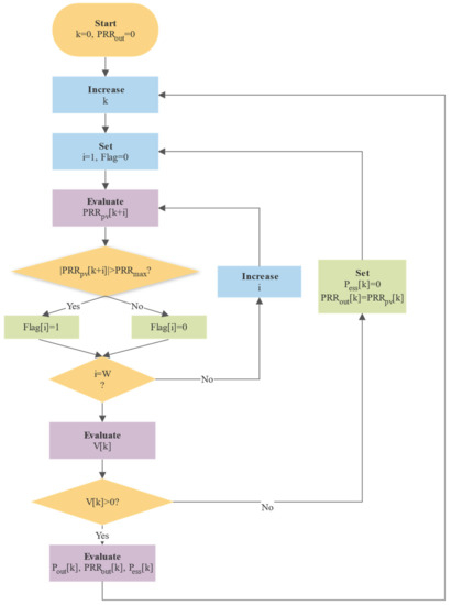
Figure 5.
Flowchart of the PDS method.
4. Methodology for the Levelized Cost of Storage Estimation
The Levelized Cost of Storage (LCOS) is an estimation of the costs associated with battery storage and is given in $/kWh/year [10,11]. The methodology to estimate the LCOS used in this work is based on the hybrid aging estimation made in [9]. This aging estimation defines the battery capacity fades associated with the storage time (calendar degradation) and with the number of complete electrical cycles of the battery (cycle degradation) for a Lithium Iron Phosphate (LFP) battery [41], which is the same battery type used in Coto Laurel:
Constants were calculated empirically. The time t is given in months and the temperature T is given in Kelvin. The number of normalized cycles NC is a compilation of the number of cycles per each DoD, which are calculated using the rainflow-counting (RFC) algorithm [9,42] and the Palmgren-Miner rule [43]. Then, the LCOS is calculated based on the estimated capacity degradation.
4.1. Battery Degradation Estimation for PRRC
The RFC algorithm counts the number of cycles per DoD. This computation is performed using the Matlab “rainflow” function, which receives the time vector with the SOC values and returns a vector with the number of cycles per DoD. The battery degradation parameter over the simulated time is obtained by using:
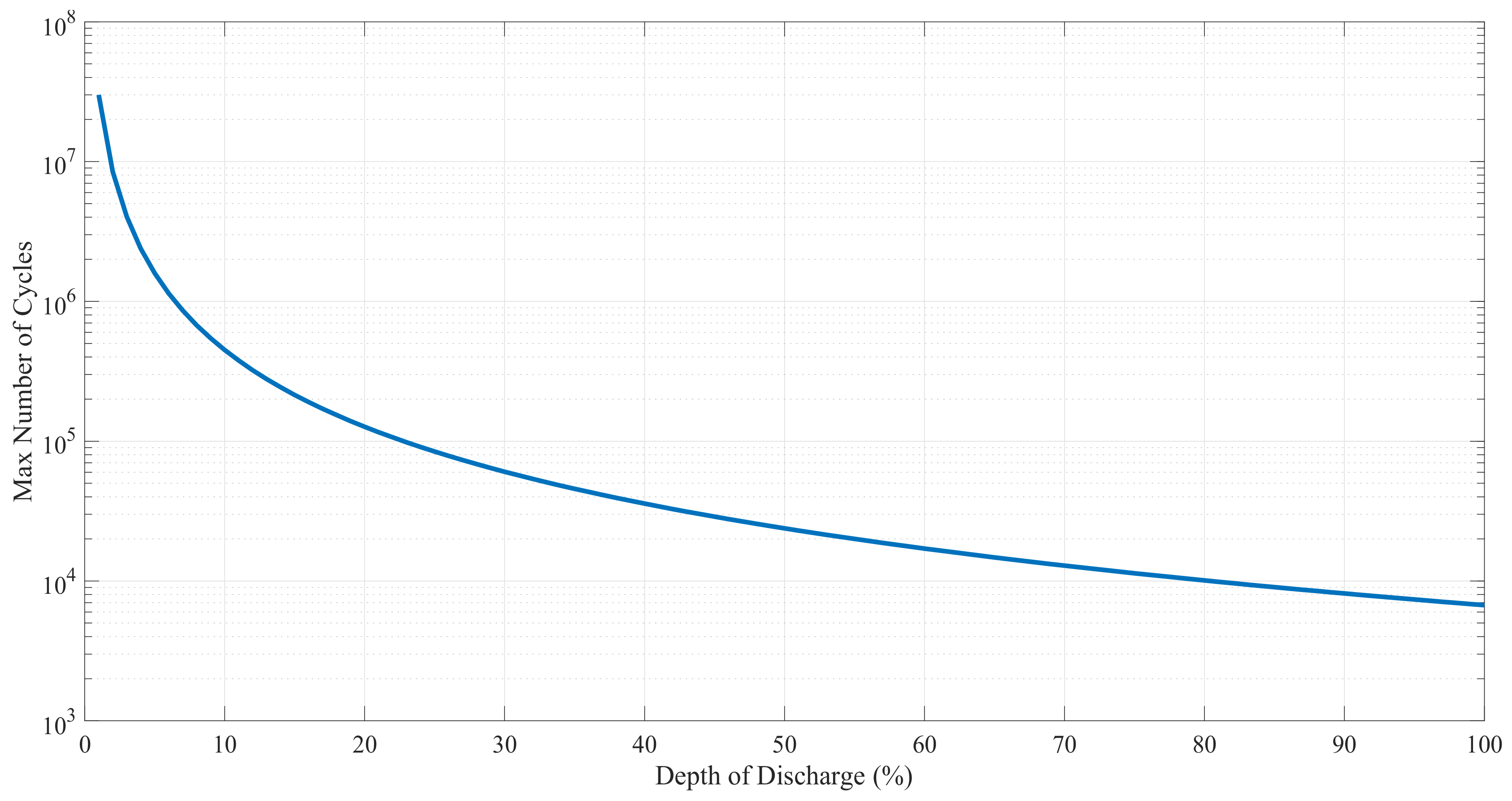
where is the maximum number of cycles per each DoD before achieving the end-of-life (EOL) and is specified by the manufacturer. Figure 6 shows the curve of against DoD for the Intensium Max High Power 20P cells LFP type from SAFT batteries, which are the battery banks used in Coto Laurel. This curve is approximated by:
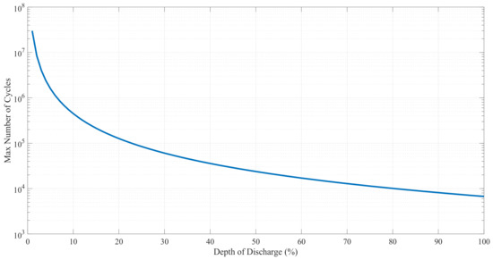
Figure 6.
Maximum number of cycles to achieve EOL for different DoD values for LFP batteries. The EOL capacity is defined by the manufacturer to be 70% of the initial capacity.
Once the overall battery degradation parameter D is obtained, it is required to transform it to a normalized number of cycles NC. Assuming a mean DoD of 80%, Figure 6 shows that the maximum number of cycles allowed before reaching the EOL is 10,000. Thus, the normalized number of cycles can be calculated using:
Then, the NC value is evaluated in (19) to obtain the capacity fade in one year. To obtain the number of years to achieve EOL considering calendar capacity fade, it is necessary to solve the following equation:
where RC is the residual capacity (70% in this case), T is the temperature and is the number of years before achieving EOL. For this work, the operating temperature is assumed constant at or .
4.2. Levelized Cost of Storage (LCOS) Estimation
The LCOS is the cost of using energy storage per year. In the case of ESS for PRRC, it is the sum of the initial battery investment and the operational costs divided by the lifetime utilization factor (LUF) [9,10]. The LUF is a time variable that considers capacity fading and AC-to-AC efficiency , which is 92% for the type of batteries used in Coto Laurel (see Section 5.1). The equation for the LCOS is defined by:
where is the initial investment of the complete ESS in $/kWh, is the operational cost assumed as 3.5% of the initial investment with a discount rate of 4%, is the remaining capacity at year y, and is the time step of the estimation in years (1 in this case) [9,10]. It can be seen from (24) that the LCOS is directly affected by the lifetime expectancy and the degradation parameter D, which are calculated using the procedure presented in the previous subsection.
4.3. Ramp Violations
Ramp violations are difficult to monetize because it varies depending on the established contract between the power company and the government. However, these violations are counted in this work to show the effectiveness of each PRRC method. The violations are counted as the cumulated measure in minutes when the PRR is above the requirements from PREPA’s MTR.
5. Coto Laurel Case Study
In this section, the Coto Laurel power plant is presented. A proposed model was developed and validated using the OP5700 simulator from Opal-RT Technologies. For this validation, the simulated data were compared against measured data from the real Coto Laurel power plant.
5.1. General Description of Coto Laurel Solar Power Plant
Coto Laurel’s PV arrays are distributed into two feeders F1 and F2, each feeder is composed of seven and eight groups, respectively. The inverters used in the Coto Laurel project for both solar panels and batteries are the “Ingecon Sun 880TL U X360 Outdoor”. For this project, a total of 21 identical inverters were used, along with 3 MWh of LFP batteries (Saft Intensium Max 20P Energy Storage Container with 8ESSUs) connected to the feeder F3. The model of the LFP batteries was developed using lookup tables based on the manufacturer’s datasheet. The technical characteristics of the ESS and the PV array are described in Table 1 and Table 2, respectively. Additionally, the one-line diagram of the solar farm is depicted in Figure 7.

Table 1.
Batteries technical data.
Table 2.
PV array technical data.
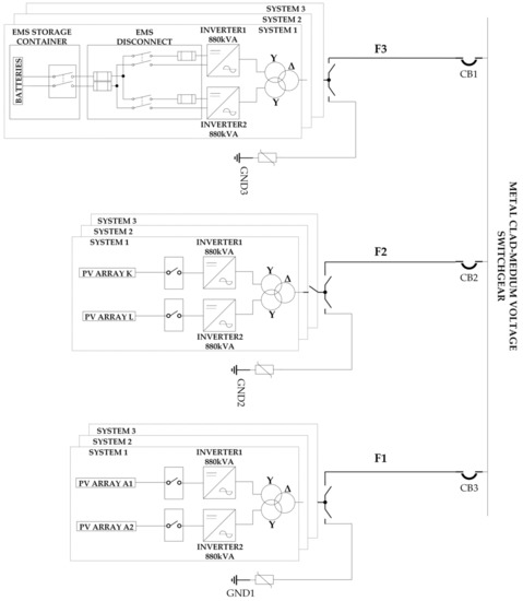
Figure 7.
One-line diagram of Coto Laurel farm.
5.2. Environmental Characteristics of Coto Laurel Solar Power Plant
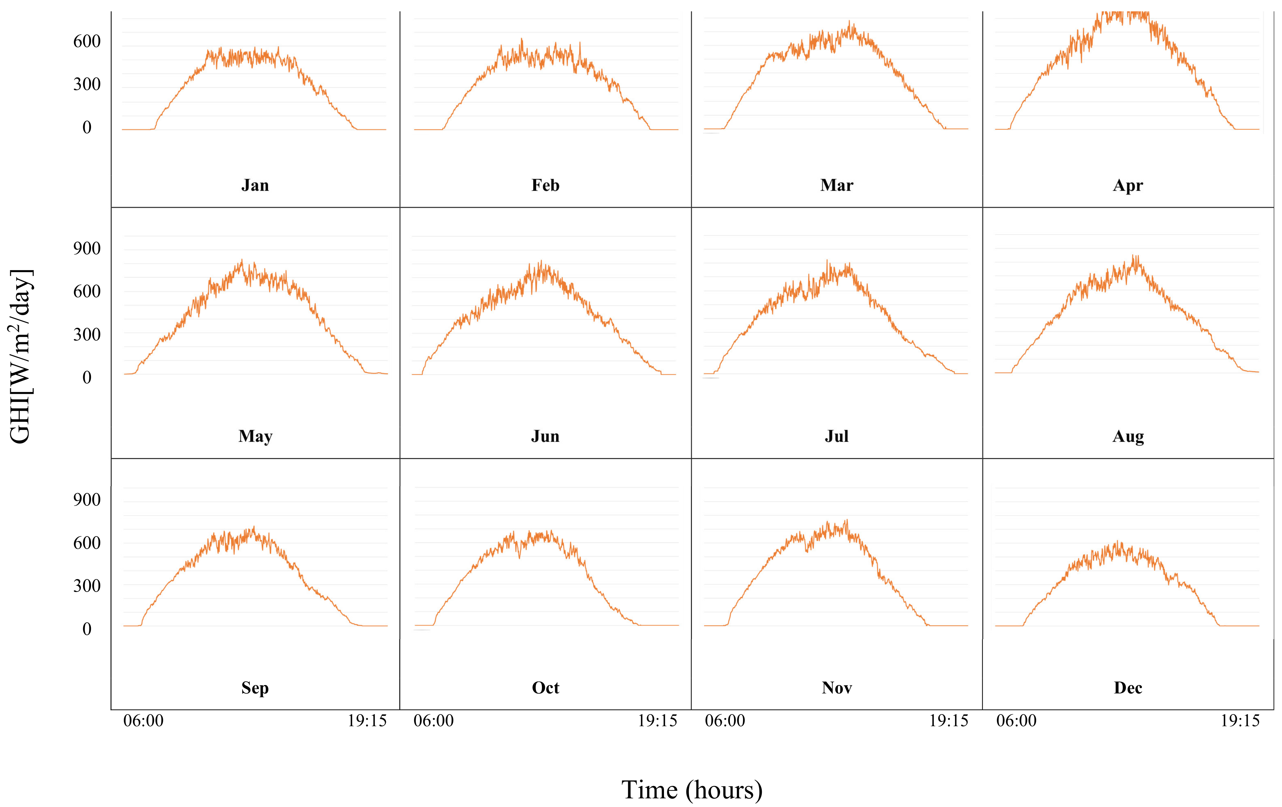
Several studies have shown that the geographic position of Puerto Rico (latitude 18°) is an excellent location for the implementation of photovoltaic plants since it receives approximately five hours of direct peak sunlight every single day of the year [44]. Additionally, Puerto Rico is in the tropical region, where no significant variations in solar irradiance can be observed throughout the year. In other words, the irradiance monthly variation is negligible as depicted in Figure 8. However, significant hourly variations can be observed throughout the day as shown in Figure 9. These hourly variations generate inconsistencies in the energy production and may generate stability issues in the main grid.
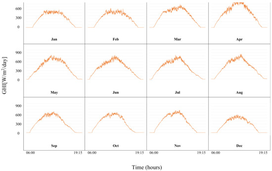
Figure 8.
Average day global horizontal irradiance (GHI) in Ponce, Puerto Rico, for each month of the year.
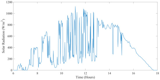
Figure 9.
Daily irradiance in Ponce, Puerto Rico on 18 May 2020.
5.3. Proposed Model
The implemented model describes the dynamics of the PV cell injection, considering the voltage of each array and the irradiance and temperature variations. The inverter was modeled as a continuous ideal AC current source. Additionally, a Direct-Quadrature (DQ) transformation was implemented to control the grid’s power injection. Finally, a phase-locked loop (PLL) was used to perform the synchronization with the grid.
The configuration of each set of arrays was carried out using the information provided by the Coto Laurel farm. The parameters of the PV panels were extracted from the corresponding solar panel’s datasheet, using information available in the standard test conditions (STD), and nominal operating cell temperature (NOCT). Additionally, the irradiance profile was measured in a meteorological station located near the system’s arrays. Moreover, the voltage of each set of arrays was obtained from the information provided by the solar farm. Using the farm’s measured parameters, a model was created using Matlab/Simulink. This model is composed of solar panels, inverters, transformers, distribution lines, and batteries.
Coto Laurel’s lithium-ion battery bank was modeled using an equivalent circuit model. This model is composed of a voltage source with a series resistor, which represents the battery’s open-circuit voltage (OCV) and internal resistance, respectively. Moreover, two RC networks in series were used to represent the electrochemical and concentration polarization of the battery. The voltage source was modeled using a lookup table that describes the relationship between the OCV and the battery level, which can be used to calculate the dynamic values of the battery’s internal resistance and the two RC networks.
Considering the nature of this study and the model’s time response (e.g., minutes), a continuous ideal AC current source was used to model the inverters on the entire system. This model is suitable for the proposed analysis since the time response of the power electronic elements and the applied current control techniques is faster (e.g., milliseconds) than the exhibited by the model. Moreover, considering the previous assumptions, a PLL with a continuous ideal AC current source was used, since it offered an accurate approximation for the current system.
The distribution and internal transmission line connections for the different elements (PV arrays, inverters, and transformers) were modeled using the branch block of the Simulink’s SimPower systems library. Moreover, a resistive three-phase branch was used to model the transmission lines available on the Coto Laurel farm, since this model provides accurate approximations for transmission lines shorter than 80 Km.
5.4. Model Validation
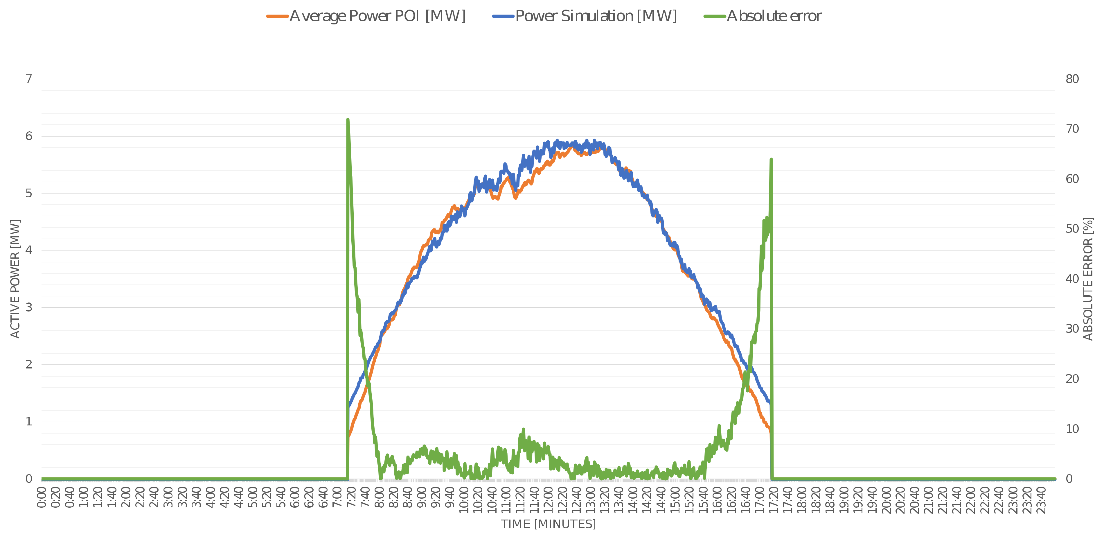
To test and validate the proposed model, a comparison between the active power calculated using the proposed model and the real data measured by the Coto Laurel’s POI’s meter was performed. To perform the simulation, the yearly average irradiance per minute was used as an input parameter. To improve accuracy and testing time, the simulation was carried out in the OP5700 simulator from Opal-RT Technologies. After running the simulation, the average power per minute was obtained, which closely matches the average power data measured at the Coto Laurel farm. Figure 10 shows the simulated mean power (blue), the measured mean power data (orange), and the absolute error (green) for each minute. The average error during the day is approximately 3.05%. It is important to highlight that at the beginning and at the end there are the highest errors of the model, this happens due to the transient that occurs in the simulation due to the change in irradiance from 0 to a certain value. However, the model demonstrates to be accurate during the rest of the day. Results from this study validate the accuracy of the model describing the dynamics of Coto Laurel.
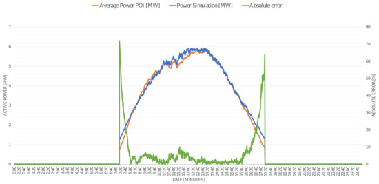
Figure 10.
Coto Laurel data vs simulation data.
6. Simulation Results
Each of the PRRC methods presented in Section 2 and Section 3 was implemented on the model presented in Section 5 using the OP5700 real-time simulator from Opal-RT Technologies. Simulation results were obtained in two stages. First, three variations of each PRRC method were evaluated for one day. The proposed PDS method was also evaluated considering variations in the prediction window and the accuracy of the prediction. In this stage, the performance indicators were the SOC variations, the SOC at the end of the day, the PRR, the PRR violations, the number of normalized cycles, the battery degradation, and the variance of the output PRR. Second, the best variation of each PRRC method was tested during an entire year to evaluate the PRR violations, the LCOS, and the degradation of the ESS.
6.1. First Stage: One Day Evaluation
The solar radiation profile used for the one-day evaluation is shown in Figure 9. This profile corresponds to 18 May 2020. This day was selected since it combines rough and smooth variations with high radiation intervals.
The same radiation profile was introduced to the modeled PV arrays shown in Figure 7. If the SOC was above 100% or below 30%, the battery banks stopped absorbing or injecting energy, respectively. The initial SOC was set to 60% to reduce the probability of reaching the SOC limits. The sampling period of all the simulations was set to 1 min.
6.1.1. Ramp Saturation Method
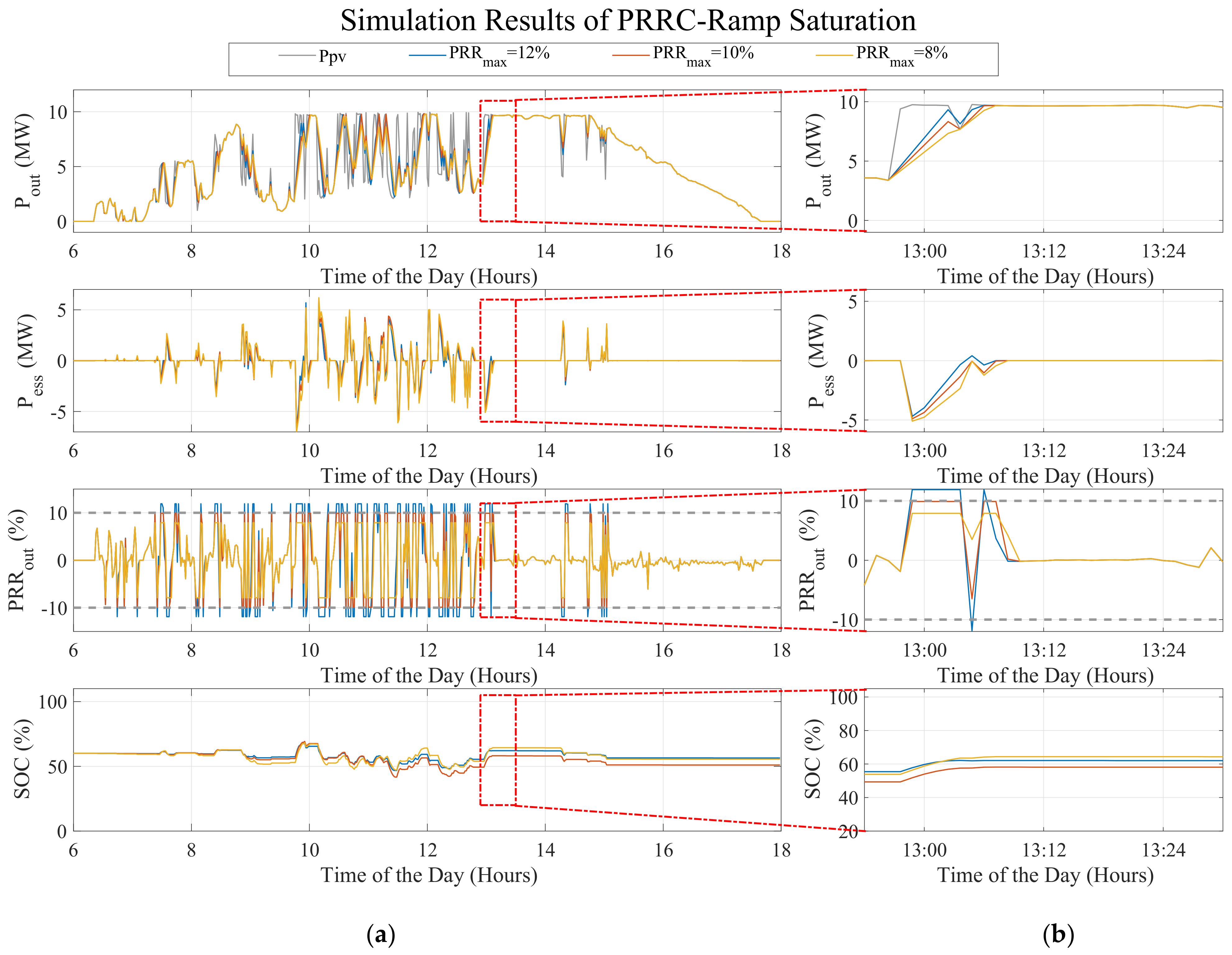
The simulation results for the RS method are shown in Figure 11. It can be noted that, as PRRmax increased, the SOC variations and the power at the ESS (Pess) were reduced. A summary of the simulation results for the RS method is shown in Table 3.
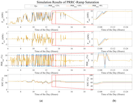
Figure 11.
Simulation results for the RS method. (a) One-day data results showing the total output power (Pout), the ESS output power (Pess), the PRR at the output (PRRout), and the state of charge (SOC). (b) Zoomed figures of the corresponding black squares.
Table 3.
Summary of the simulation results for the RS method.
6.1.2. Simple Moving Average (SMA) Method
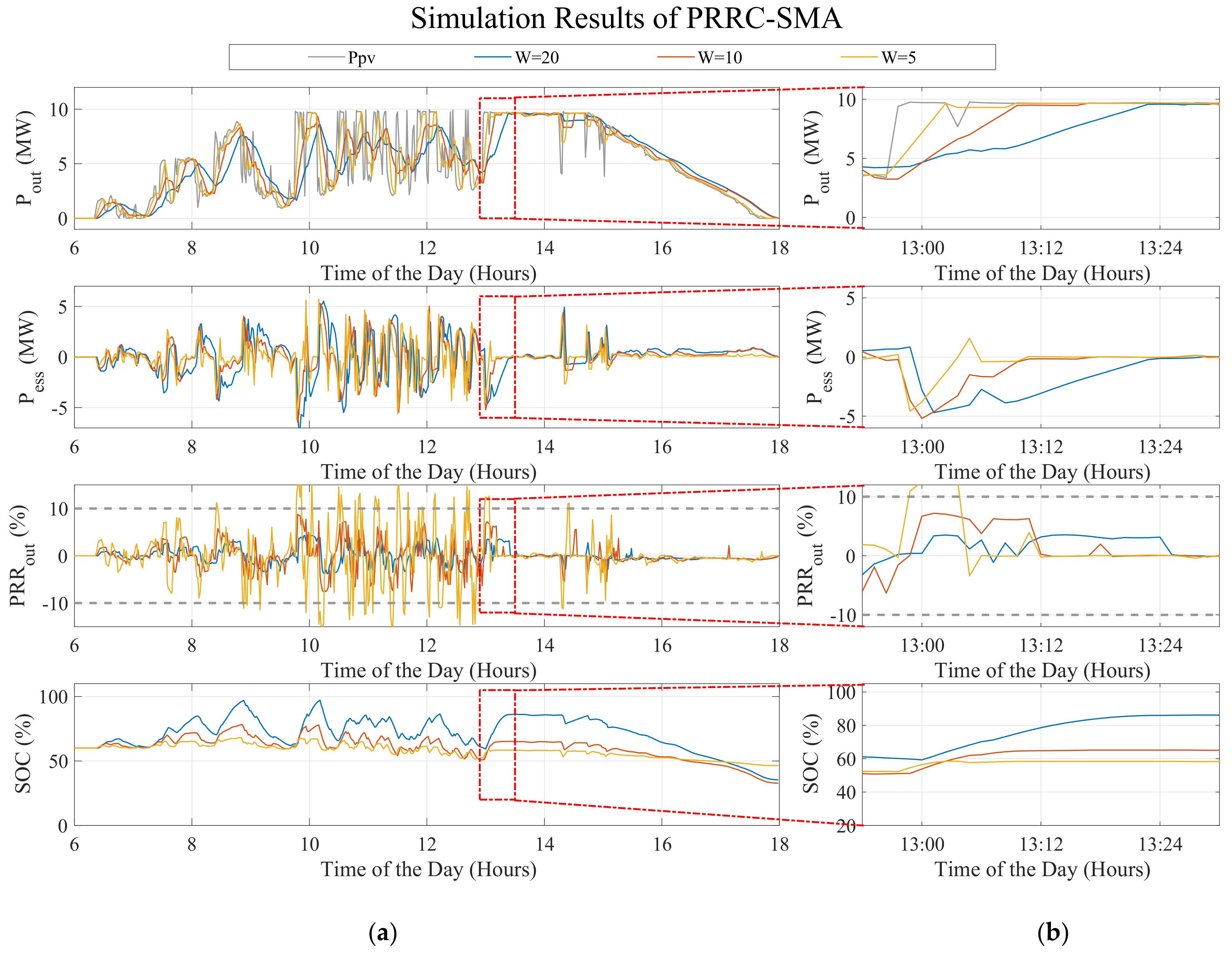
Simulation results for the SMA are shown in Figure 12. It is noted that, as the window size is increased, the output PRR is reduced and the SOC variations increase. A summary of the simulation results for the RS method is shown in Table 4. A window size of W = 10 causes half of the degradation compared to W = 20. Furthermore, the variance of PRRout for W = 10 is more than three times less than W = 5.
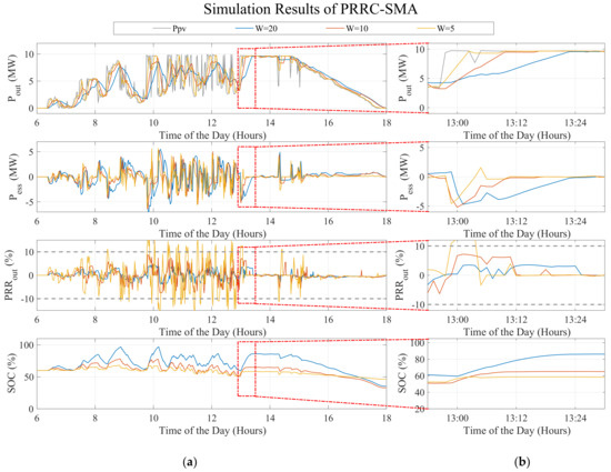
Figure 12.
Simulation results for the SMA method. (a) One-day data results showing the total output power (Pout), the ESS output power (Pess), the PRR at the output (PRRout), and the state of charge (SOC). (b) Zoomed figures of the corresponding black squares.
Table 4.
Summary of the simulation results for the SMA method.
6.1.3. Exponential Moving Average (EMA) Method
Simulation results for the EMA method are presented in Figure 13. All the simulations were made using a window size of 30. Although output and ESS powers are similar for each , it is noted that the SOC reached 100% at t = 13:12 for . Thus, the ESS stopped absorbing energy and PRR violations started to appear. A summary of the simulation results for the RS method is shown in Table 5. There are no violations with since it has the least PRR variance in all three tests.
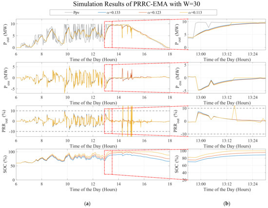
Figure 13.
Simulation results for the EMA method. (a) One-day data results showing the total output power (Pout), the ESS output power (Pess), the PRR at the output (PRRout), and the state of charge (SOC). (b) Zoomed figures of the corresponding black squares.
Table 5.
Summary of the simulation results for the EMA method.
6.1.4. First Order Low-Pass Filter (FOLPF) Method
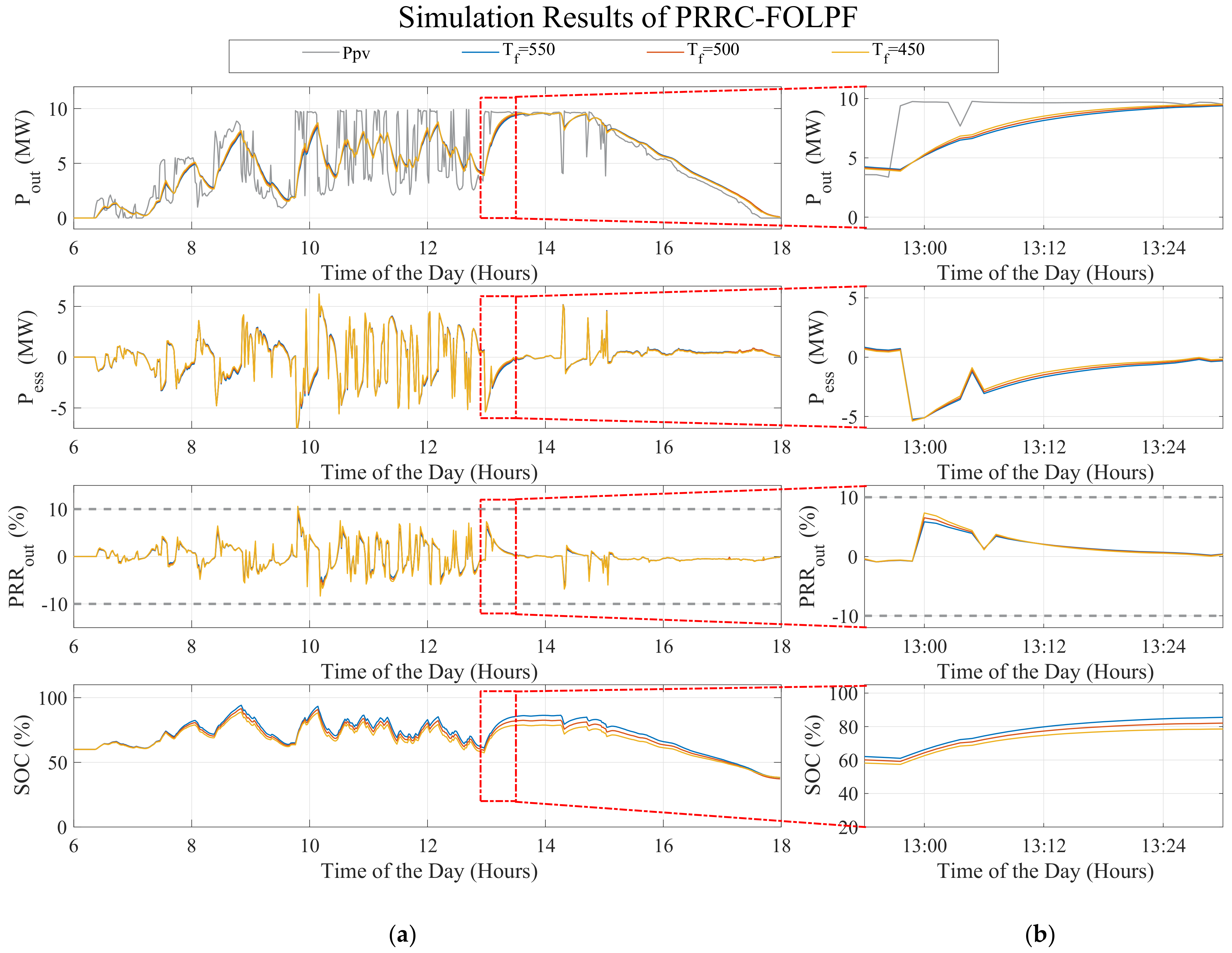
Simulation results for the FOLPF method are shown in Figure 14. It is noted that, although results were similar, there was a violation at t = 10:15 for = 450. A summary of the simulation results for the FOLPF method is shown in Table 6. The least degradation without having PRR violations occurred when .
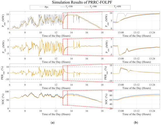
Figure 14.
Simulation results for the FOLPF method. (a) One-day data results showing the total output power (Pout), the ESS output power (Pess), the PRR at the output (PRRout), and the state of charge (SOC). (b) Zoomed figures of the corresponding black squares.
Table 6.
Summary of the simulation results for the FOLPF method.
6.1.5. Second Order Low-Pass Filter (SOLPF) Method
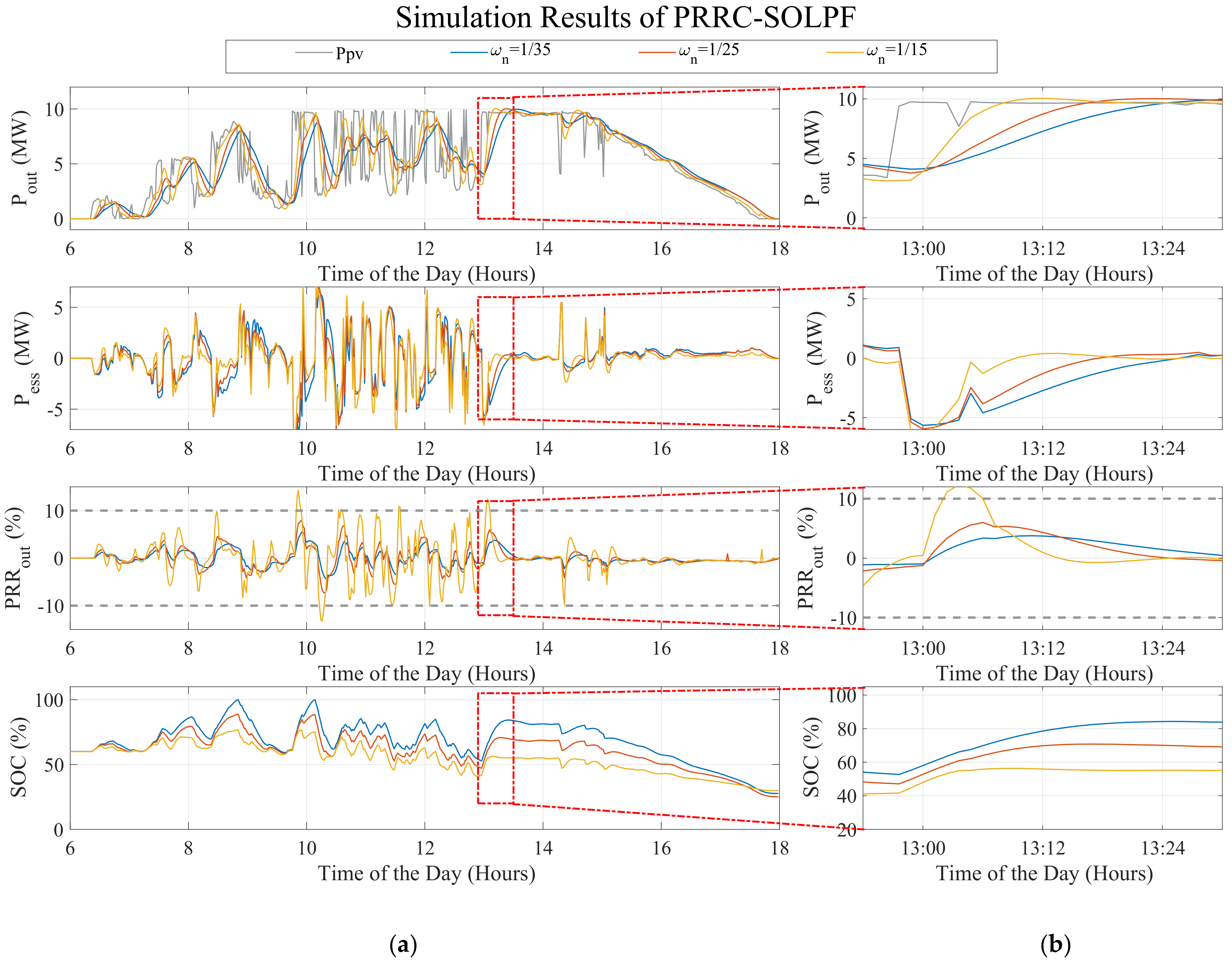
Simulation results for the SOLPF method are shown in Figure 15. It is noted that the SOC reached the upper limit twice during the day for = 1/35. Furthermore, there were multiple violations for = 1/35. A summary of the simulation results for the SOLPF method is shown in Table 7. The least degradation without having PRR violations occurred when .
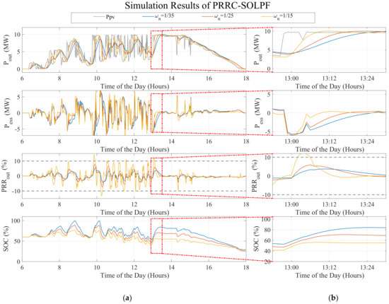
Figure 15.
Simulation results for the SOLPF method. (a) One-day data results showing the total output power (Pout), the ESS output power (Pess), the PRR at the output (PRRout), and the state of charge (SOC). (b) Zoomed figures of the corresponding black squares.
Table 7.
Summary of the simulation results for the SOLPF method.
6.1.6. Enhanced Linear Exponential Smoothing (ELES) Method
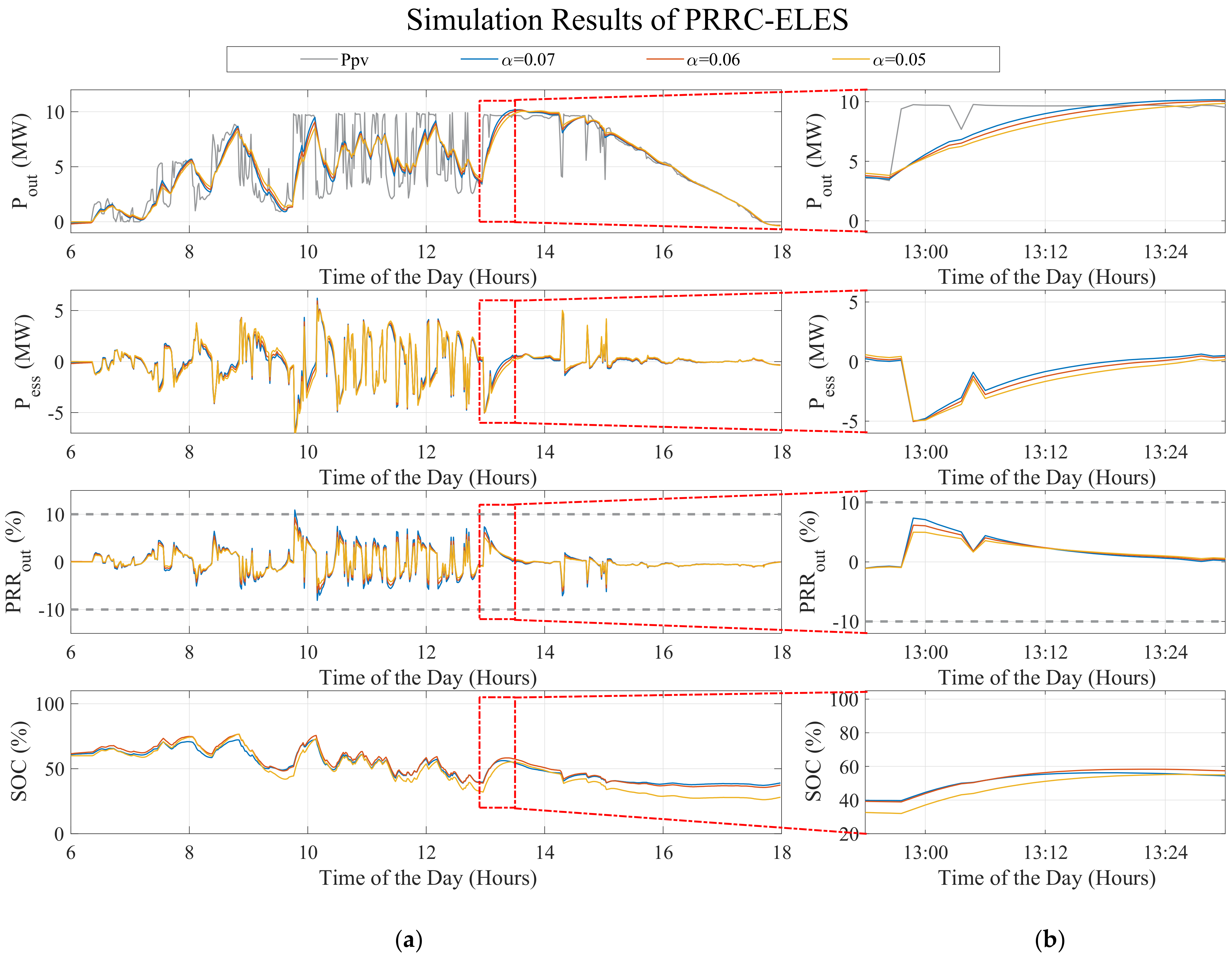
Simulation results for the ELES method are shown in Figure 16. It is noted that, although results were similar, there was a violation at t = 9:50 for = 0.07. A summary of the simulation results for the ELES method is shown in Table 8. The least degradation without having PRR violations occurred when .
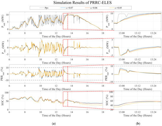
Figure 16.
Simulation results for the ELES method. (a) One-day data results showing the total output power (Pout), the ESS output power (Pess), the PRR at the output (PRRout), and the state of charge (SOC). (b) Zoomed figures of the corresponding black squares.
Table 8.
Summary of the simulation results for the ELES method.
6.1.7. Proposed Predictive Dynamic Smoothing (PDS)
The PDS was evaluated by varying the prediction window size W (5 and 10). However, since this method relies on the accuracy of the predictions, its robustness against prediction inaccuracies was also evaluated. For this purpose, the assumed prediction was contaminated with Gaussian noise as follows:
where rand is a random scalar with standard normal distribution and is the variable noise parameter in the percent of the contracted output power. This means that a incurred in an estimated power estimation error of approximately 2 MW.
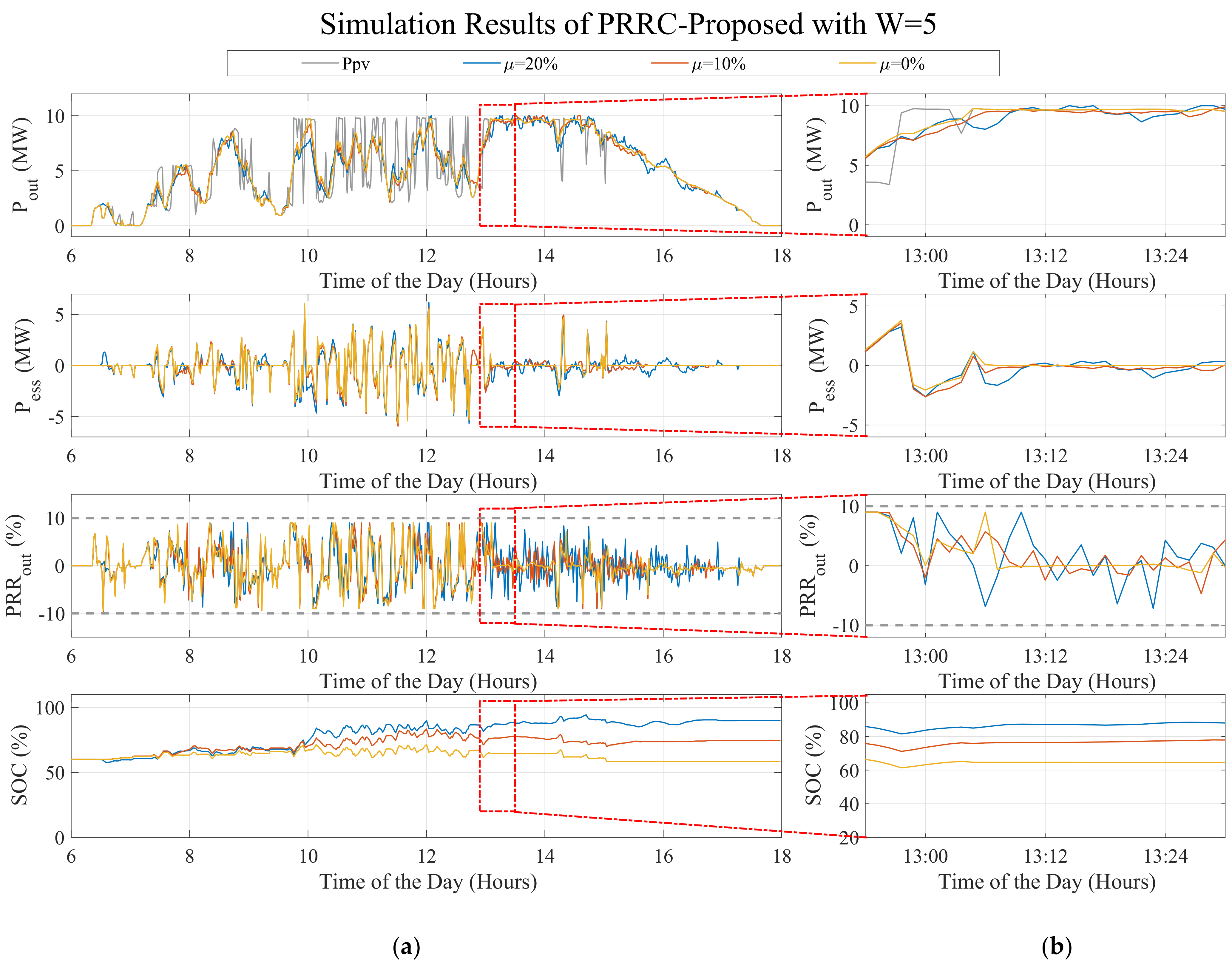
Simulation results for the PDS method with W = 5 are shown in Figure 17. It is noted that, compared to other methods, the SOC variations got reduced and there were no PRR violations. It is also noted that the SOC variations are critically affected by the parameter. A summary of these results is presented in Table 9. The PDS shows to be robust against an estimation noise of at least 20%. The battery degradation is also small compared to other methods.
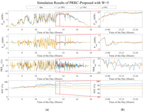
Figure 17.
Simulation results for the proposed PDS method. (a) One day data results showing the total output power (Pout), the ESS output power (Pess), the PRR at the output (PRRout), and the state of charge (SOC). (b) Zoomed figures of the corresponding black squares.
Table 9.
Summary of the simulation results for the proposed PDS method with W = 5.
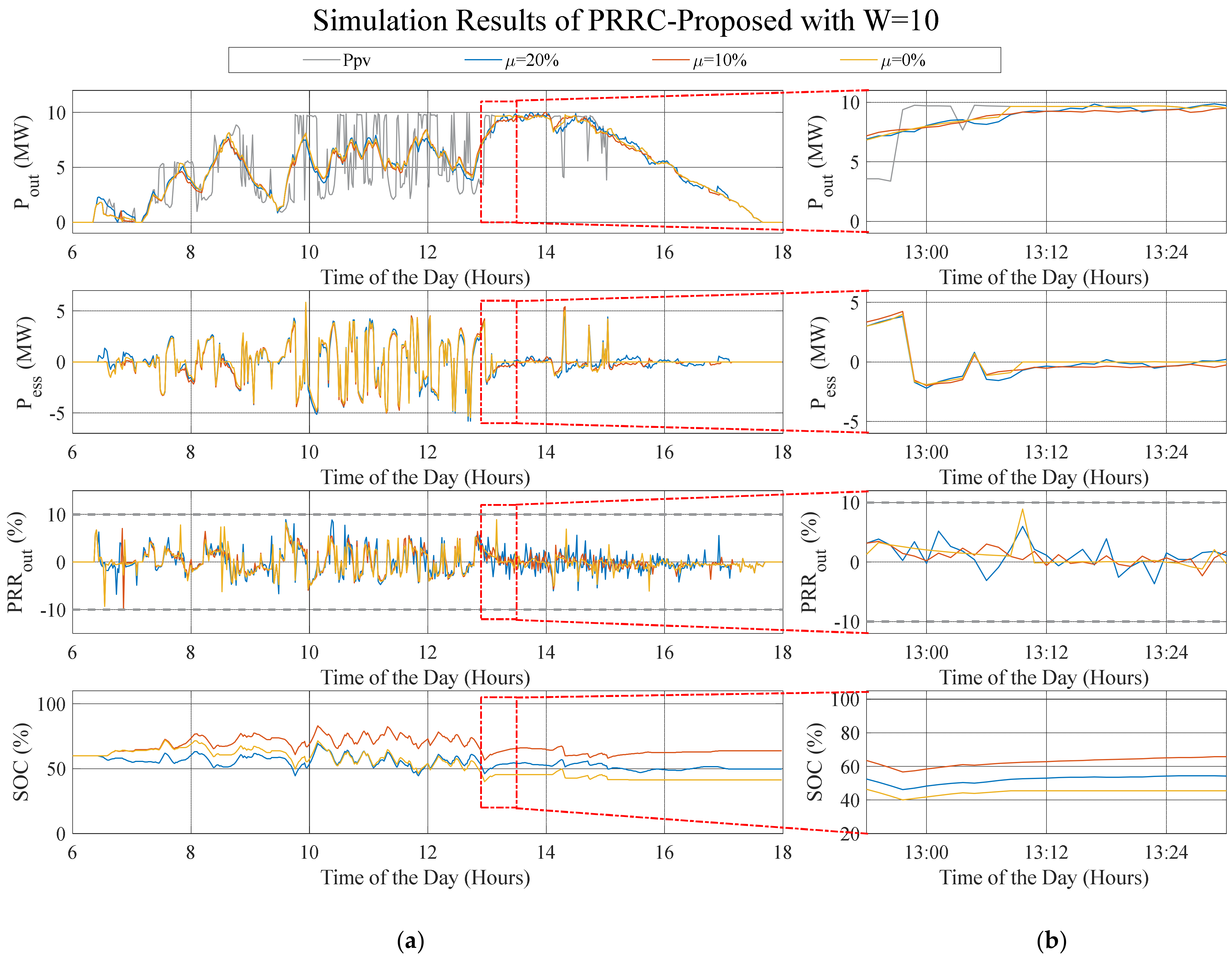
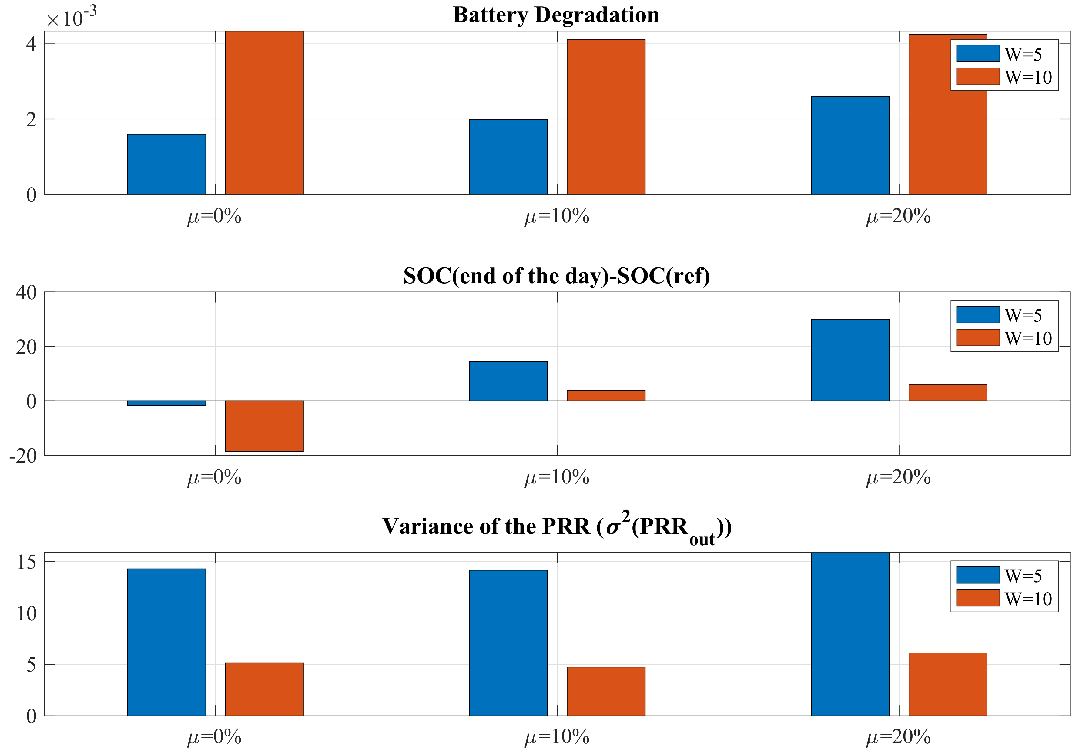
Simulation results for the PDS method with W = 10 are shown in Figure 18. It is noted that this window size significantly reduced the PRR and SOC variations. It is concluded that, as the window size increases, the PDS is more robust against uncertainties in the predictions. It is also noted that the SOC variations are critically affected by the parameter. A summary of these results is presented in Table 10. Although none of the tests showed PRR violations and the PRR variance was significantly reduced, a PDS method with a W = 10 showed twice the battery degradation compared with a window size of W = 5. Figure 19. Comparison of the effect of selecting the window size using the PDS method. Figure 19 shows the main effects of selecting the window size.
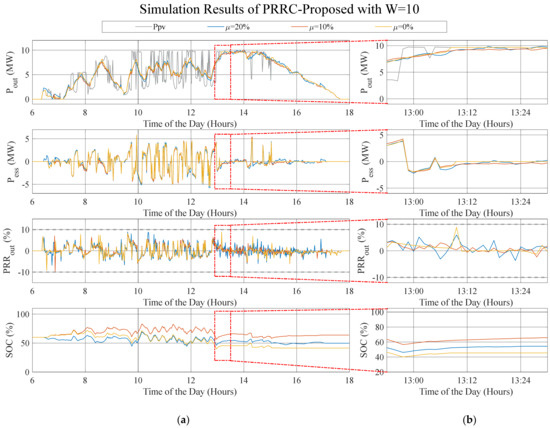
Figure 18.
Simulation results for the proposed PDS method. (a) One-day data results showing the total output power (Pout), the ESS output power (Pess), the PRR at the output (PRRout), and the state of charge (SOC). (b) Zoomed figures of the corresponding black squares.
Table 10.
Summary of the simulation results for the proposed PDS method with W = 10.
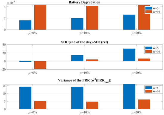
Figure 19.
Comparison of the effect of selecting the window size using the PDS method.
6.2. Economic Analysis through One Year
From the previous subsection, one parameter configuration was selected for each PRRC method to be tested using a whole year’s data. These configurations were selected considering the minimum amount of degradation without having PRR violations. Additionally, the mean of the SOC and the variance of the output PRR were considered. The SOC at the end of the day is an indicator of SOC variations and is also used as a selection criterion. With these criteria in mind, the following PRRC methods were considered for this section:
- RS with a PRRmax of 10%.
- SMA with a window size W = 10.
- EMA with a window size W = 30 and a smoothing factor α = 0.123.
- FOLPF with a sampling period Ts = 60 s and a Tf = 500 s.
- SOLPF with a sampling period of Ts = 60 s, a damping ratio ζ = 0.707, and a natural frequency ωn = 1/25 rad/s.
- ELES with a smoothing factor α = 0.06.
- Proposed PDS with a window size W = 5 and a disturbance coefficient µ = 10%. This coefficient was selected since it represented errors in estimations of about 1 MW, which is reasonable according to the literature presented in Section 3.
First, a battery degradation analysis was made to each of the PRRC methods. Then, the estimated cost per kWh per year was compared. Finally, the violations throughout the year were analyzed. The solar radiation data for this test was selected from 20 May 2019 to 19 May 2020. Results were summarized at the end of this section. It is important to mention that, as the SOC at the end of each day is not the same as the one at the beginning of the day, the mean SOC tended to drift during the year until it reached the maximum or minimum limits. To account for this issue, a proportional SOC controller was added at the output of each PRRC controller. The mathematical expression for this controller is dictated by:
where is the adjusted power reference for the ESS, is the output of the PRRC method, is the desired SOC at the end of the day, and is the proportional control constant, which is selected small to not affect the dynamics of the PRRC.
6.2.1. Battery Degradation
The summarized number of cycles using the rainflow algorithm are depicted in Figure 20. The cycles are a histogram representing the number of cycles per DoD during an entire year for the Coto Laurel plant under different PRRC methods using the rainflow algorithm. The DoDs were accumulated in intervals of 10%. With this information, it was possible to determine the capacity degradation and the lifetime of the ESS by using (18)–(23) with a temperature of and an estimated end-of-life (EOL) capacity of 70%, according to the manufacturer.
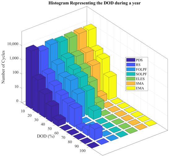
Figure 20.
Histogram representing the number of cycles per each DoD during an entire year for the Coto Laurel plant under different PRRC methods using the rainflow algorithm. The DoDs were accumulated in intervals of 10%.
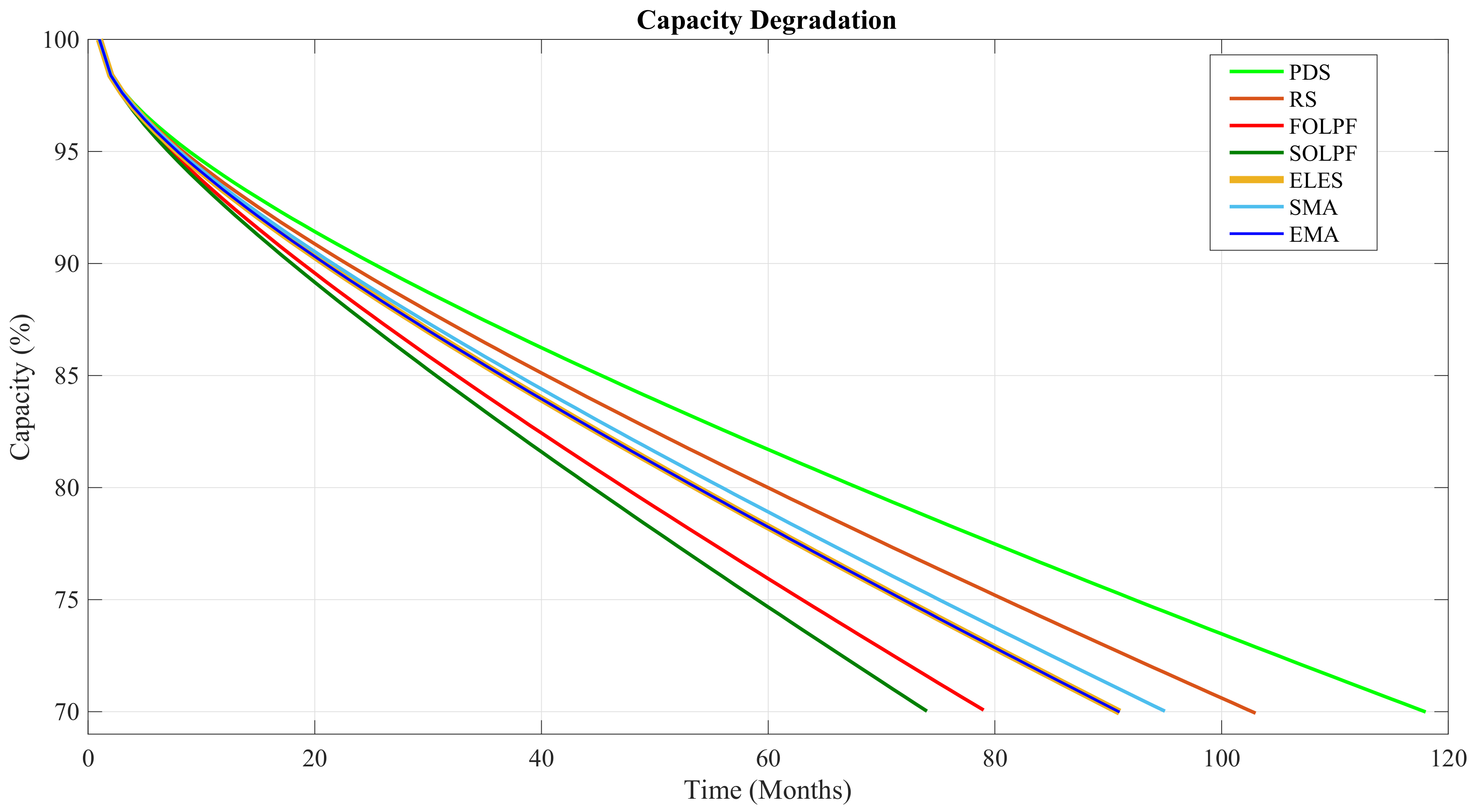
According to Figure 21, The PDS showed to be the PRRC method that offers the most estimated battery lifetime (118 months), followed by the RS (103 months), the SMA (95 months), the ELES and EMA (91 months), the FOLPF (79 months), and the SOLPF (74 months). This was because the PDS method produced fewer battery cycles for high DoD values. According to Figure 6, the battery life is exponentially affected as the number of cycles of high DoD values increase.
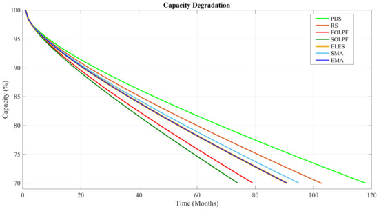
Figure 21.
ESS capacity degradation estimation using a whole year data from Coto Laurel simulations under different PRRC methods.
6.2.2. LCOS
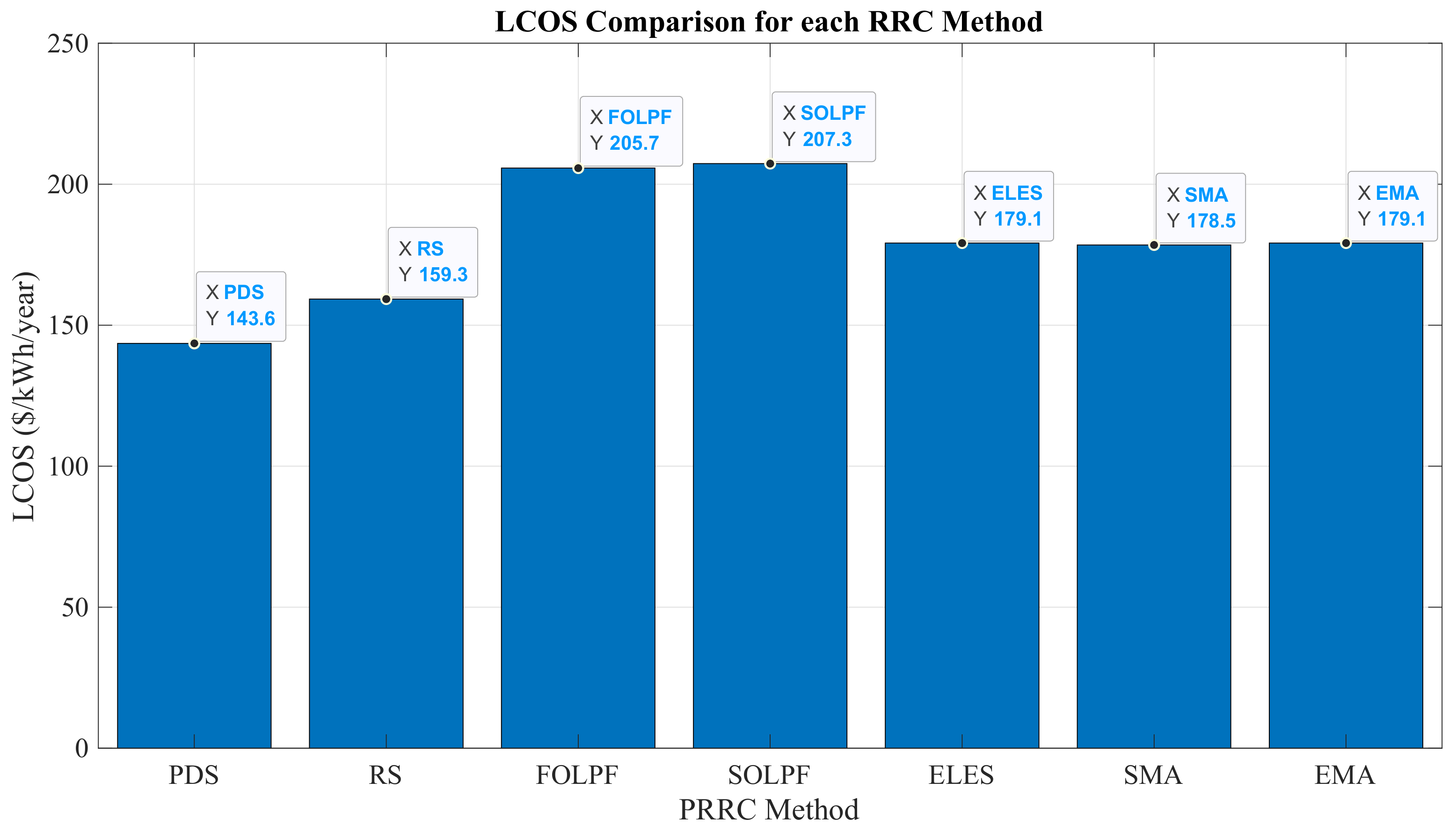
The initial investment for the LCOS analysis was determined based on [9], which used as base various reports from international technology centers and specialized consultancies. According to this, the estimated initial investment for a 3 MWh LFP ESS is about 2.35M€ or 2.87M$ (USD as of May 2021 exchange rate). Figure 22 shows a comparison of the LCOS (in $/kWh/year) for each PRRC method. These results were obtained using (24). These results were consistent with those presented in Figure 21.
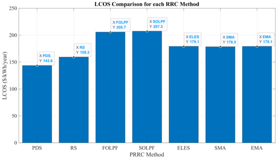
Figure 22.
Comparison of the LCOS for each PRRC method. This analysis was based on data from an entire year in the Coto Laurel power plant.
Results from Figure 22 indicate that the LCOS is highly dependent on battery degradation, which directly affects the battery lifetime and the capacity degradation of the ESS. One of the main advantages of the proposed PDS is that the DoD is considerably reduced by charging or discharging the ESS before a PRR event arrives. This also helps to reduce cumulated SOC drifts throughout the year. In order to increase battery lifetime, it is also recommended to reduce the amplitude of the SOC fluctuations. Furthermore, it is important to consider the penalties for violating the PRR requirements. This must be considered along with the LCOS to decide which PRRC method is more convenient for a particular LSSPP.
6.2.3. Violations
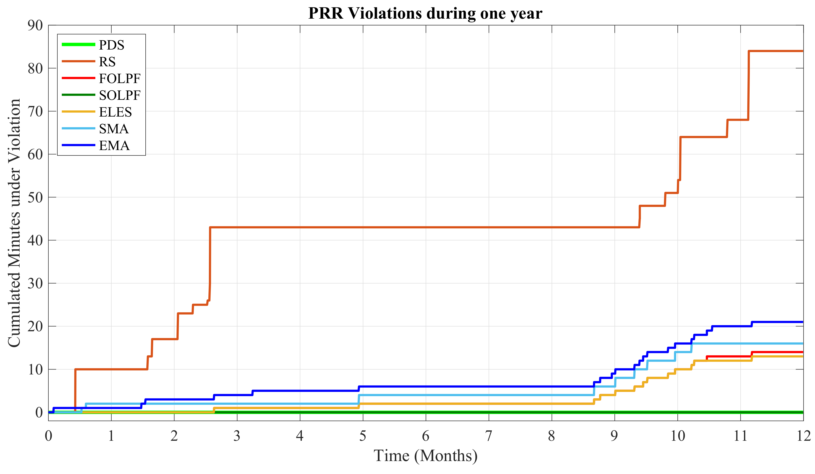
It is difficult to assign a monetary value to the PRR violations since this is unique for each agreement. However, PRR violations throughout the year are presented in this work to serve as an indicator of the accuracy and performance of each PRRC method. Figure 23 shows the cumulated measurement of the minutes when the output PRR was greater than PRRmax. It is noted that most of the PRR violations in Coto Laurel occurred during the summer, which is characterized for having the highest solar radiation profiles according to Figure 8. The main cause of these violations over the year was because the ESS reached its minimum (30%) or maximum capacity (100%). This implied that the ESS was unable to support the PRRC. However, the PRR violations were relatively small, considering that the RS was the PRRC method with the most violations throughout the year (84 min). The PDS and the SOLPF were the PRRC methods that did not show any PRR violations throughout the year.
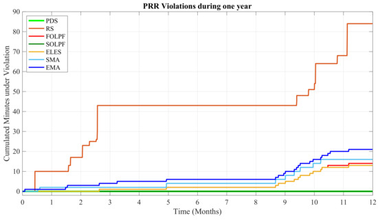
Figure 23.
Cumulated minutes when the output PRR violated the requirements.
7. Discussion
The model of the Coto Laurel solar power plant was developed, tested, and validated using an OP5700 simulator from OPAL-RT technologies. Simulation results throughout the year validated the accuracy of the proposed Coto Laurel model. With this model, a novel PRRC method was proposed. This proposed method and other PRRC methods were tested using daily and yearly data. Daily results indicate that there is a tradeoff between PRR regulation and DoD cycles. It is important to determine the storage capacity required to optimize PRR support and battery degradation. For this work, the marginal required storage capacity was used. However, less degradation could be appreciated when this capacity is increased. Furthermore, as the storage capacity is increased, the PRR violations are expected to decrease. This is because it is less probable to reach the minimum or maximum SOC values. When this event occurs, mainly during summer, the PRRC method is unable to support the PRR regulation.
Among the PRRC methods found in the literature, the RS showed to be the one with the least LCOS value. However, there are some days when the ESS may reach the maximum or minimum value, limiting the capacity of the RS method to support the PRRC. The ELES, SMA, and EMA showed similar LCOS values. However, the EMA showed the most violations of these three methods. Although the SOLPF did not show PRR violations, it is the PRRC method with the highest LCOS, followed by the FOLPF.
The proposed PDS method showed the least LCOS values among all the PRRC methods. This was because the PDS used predicted data to charge or discharge the ESS to reduce DoD. This helped to reduce high-valued DoD cycles, which considerably increased the battery life while regulating the PRR without violations. Moreover, the PDS demonstrated to be robust against solar prediction inaccuracies of at least 20% of the real value with a minimum prediction window of 5 min. At shorter sampling periods, the algorithm would have more resolution correcting sudden PV power drops. However, if the window size is not increased, more violations would be expected, and the degradation would decrease because the ESS will not be used frequently because their output will not be smoothed. It is important to note that the selection of the sampling period was made based on the regulations, which dictated the PRR limit in minutes.
It is important to consider that the predictive nature of the PDS may incur extra costs depending on the selected prediction method. There are plenty of solar prediction methods available in the literature that may be used for the PDS implementation [6,35,36,39,40]. However, it is important to consider the accuracy, the costs, and the effectiveness of these methods against radiation profiles found in places such as Puerto Rico. As future work, it is of interest to study the complete implementation of the PDS method in a real solar power plant using one of the solar prediction methods found in the literature.
Author Contributions
Conceptualization, J.F.P.-M.; methodology, J.F.P.-M., J.D.V.-P., Y.V.G. and O.F.R.-M.; software, J.D.V.-P., Y.V.G. and O.F.R.-M.; validation, J.D.V.-P., Y.V.G. and O.F.R.-M.; formal analysis, J.F.P.-M.; resources, F.A.; writing—original draft preparation, J.F.P.-M., Y.V.G. and O.F.R.-M.; writing—review and editing, J.F.P.-M. and F.A.; supervision, F.A.; funding acquisition, F.A. All authors have read and agreed to the published version of the manuscript.
Funding
This work was supported by the U.S. Department of Energy under Grant DE-SC0020281.
Institutional Review Board Statement
Not applicable.
Informed Consent Statement
Not applicable.
Data Availability Statement
The data available in this study is openly available in IEEE Dataport, doi:10.21227/kkj4-fh6.
Acknowledgments
Special thanks to Víctor González, from Windmar LLC, for providing the power data and system description used in this article.
Conflicts of Interest
The authors declare no conflict of interest. The funders had no role in the design of the study; in the collection, analyses, or interpretation of data; in the writing of the manuscript, or in the decision to publish the results.
References
- Puerto Rico Electrical Power Authority. Generation, Consumption, Cost, Income and Customers of the Puerto Rico Electrical System; indicadores.pr: San Juan, PR, USA, 2020. [Google Scholar]
- Puerto Rico Electric Power Authority. SB 1121 Puerto Rico Energy Public Policy Act; Government of Puerto Rico: San Juan, PR, USA, 2020; p. 23.
- Government of Puerto Rico. PREPA Hydroelectric Power Plants Revitalization Project (PRQ2019-2)—Questions and Responses Log; Government of Puerto Rico: San Juan, PR, USA, 2020.
- Puerto Rico Energy Bureau. Final Resolution and Order on the Puerto Rico Electric Power Authority’s Integrated Resource Plan (CEPR-AP-2018-0001); Puerto Rico’s Electric Energy Bureau: San Juan, PR, USA, 2020; p. 179.
- Crǎciun, B.I.; Kerekes, T.; Séra, D.; Teodorescu, R.; Annakkage, U.D. Power Ramp Limitation Capabilities of Large PV Power Plants With Active Power Reserves. IEEE Trans. Sustain. Energy 2017, 8, 573–581. [Google Scholar] [CrossRef]
- Martins, J.; Spataru, S.; Sera, D.; Stroe, D.I.; Lashab, A. Comparative study of ramp-rate control algorithms for PV with energy storage systems. Energies 2019, 12, 1342. [Google Scholar] [CrossRef] [Green Version]
- Elwakil, E.; Hegab, M. Risk Management for Power Purchase Agreements. In Proceedings of the 2018 IEEE Conference on Technologies for Sustainability (SusTech), Long Beach, CA, USA, 11–13 November 2018. [Google Scholar] [CrossRef]
- Puerto Rico Electric Power Authority. Minimum Technical Requirements For Interconnection Of Photovoltaic (Pv) Facilities; Energia.pr.gov: San Juan, PR, USA, 2020; pp. 1–11.
- Beltran, H.; Tomas Garcia, I.; Alfonso-Gil, J.C.; Perez, E. Levelized Cost of Storage for Li-Ion Batteries Used in PV Power Plants for Ramp-Rate Control. IEEE Trans. Energy Convers. 2019, 34, 554–561. [Google Scholar] [CrossRef]
- Belderbos, A.; Delarue, E.; D’haeseleer, W. Calculating the levelized cost of storage? Energy Expect. In Proceedings of the Uncertainty, 39th IAEE International Conference, Beren, Norway, 19–22 November 2016; pp. 1–2. [Google Scholar]
- Hoff, M.; Lin, R. Development and Practical Use of a Levelized Cost of Storage (LCOS) Metric. Available online: https://www.neces.com/wp-content/uploads/2019/08/Development_and_practical_use_of_a_LCOS_031619.pdf (accessed on 27 January 2021).
- Alam, M.J.E.; Muttaqi, K.M.; Sutanto, D. A novel approach for ramp-rate control of solar PV using energy storage to mitigate output fluctuations caused by cloud passing. IEEE Trans. Energy Convers. 2014, 29, 507–518. [Google Scholar] [CrossRef] [Green Version]
- Marcos, J.; de La Parra, I.; García, M.; Marroyo, L. Control strategies to smooth short-term power fluctuations in large photovoltaic plants using battery storage systems. Energies 2014, 7, 6593–6619. [Google Scholar] [CrossRef]
- Solanki, S.G.; Ramachandaramurthy, V.K.; Shing, N.Y.K.; Tan, R.H.G.; Tariq, M.; Thanikanti, S.B. Power smoothing techniques to mitigate solar intermittency. In Proceedings of the 2019 International Conference on Electrical, Electronics and Computer Engineering, UPCON 2019, Aligarh, India, 8–10 November 2019. [Google Scholar]
- Tesfahunegn, S.G.; Ulleberg, Ø.; Vie, P.J.S.; Undeland, T.M. PV fluctuation balancing using hydrogen storage—A smoothing method for integration of PV generation into the utility grid. Energy Procedia 2011, 12, 1015–1022. [Google Scholar] [CrossRef] [Green Version]
- Ellis, A.; Schoenwald, D.; Hawkins, J.; Willard, S.; Arellano, B. PV output smoothing with energy storage. In Proceedings of the Conference Record of the IEEE Photovoltaic Specialists Conference, Austin, TX, USA, 3–8 June 2012; pp. 1523–1528. [Google Scholar]
- Hund, T.D.; Gonzalez, S.; Barrett, K. Grid-tied PV system energy smoothing. In Proceedings of the Conference Record of the IEEE Photovoltaic Specialists Conference, Honolulu, HI, USA, 20–25 June 2010; pp. 2762–2766. [Google Scholar]
- Addisu, A.; George, L.; Courbin, P.; Sciandra, V. Smoothing of renewable energy generation using Gaussian-based method with power constraints. Energy Procedia 2017, 134, 171–180. [Google Scholar] [CrossRef]
- Lin, D. Strategy Comparison of Power Ramp Rate Control for Photovoltaic Systems. CPSS Trans. Power Electron. Appl. 2020, 5, 329–341. [Google Scholar] [CrossRef]
- Jamroen, C.; Usaratniwart, E.; Sirisukprasert, S. PV power smoothing strategy based on HELES using energy storage system application: A simulation analysis in microgrids. IET Renew. Power Gener. 2019, 13, 2298–2308. [Google Scholar] [CrossRef]
- Chanhom, P.; Sirisukprasert, S.; Hatti, N. Enhanced linear exponential smoothing technique with minimum energy storage capacity for PV distributed generations. Int. Rev. Electr. Eng. 2014, 9, 1190–1196. [Google Scholar] [CrossRef]
- Usaratniwart, E.; Sirisukprasert, S.; Hatti, N.; Hagiwara, M. A case study in micro grid using adaptive enhanced linear exponential smoothing technique. In Proceedings of the 2017 8th International Conference on Information and Communication Technology for Embedded Systems, IC-ICTES 2017—Proceedings, Chonburi, Thailand, 7–9 May 2017. [Google Scholar]
- Usaratniwart, E.; Sirisukprasert, S. Adaptive enhanced linear exponential smoothing technique to mitigate photovoltaic power fluctuation. In Proceedings of the IEEE PES Innovative Smart Grid Technologies Conference Europe, Melbourne, VIC, Australia, 28 November–1 December 2016; pp. 712–717. [Google Scholar]
- Liu, H.; Peng, J.; Zang, Q.; Yang, K. Control Strategy of Energy Storage for Smoothing Photovoltaic Power Fluctuations. IFAC-PapersOnLine 2015, 48, 162–165. [Google Scholar] [CrossRef]
- Datta, M.; Senjyu, T.; Yona, A.; Funabashi, T.; Kim, C.H. Photovoltaic output power fluctuations smoothing methods for single and multiple PV generators. Curr. Appl. Phys. 2010, 10, S265–S270. [Google Scholar] [CrossRef]
- Koiwa, K.; Liu, K.Z.; Tamura, J. Analysis and Design of Filters for the Energy Storage System: Optimal Tradeoff between Frequency Guarantee and Energy Capacity/Power Rating. IEEE Trans. Ind. Electron. 2018, 65, 6560–6570. [Google Scholar] [CrossRef]
- Lin, Z.; Qiu, G.; Wang, G.; Jiang, R. Improved wind power and storage system smoothing control strategy based on RE reinforcement learning and low pass filtering algorithms. In Proceedings of the POWERCON 2014–2014 International Conference on Power System Technology: Towards Green, Efficient and Smart Power System, Chengdu, China, 20–22 October 2014; pp. 1749–1753. [Google Scholar]
- Nikolov, D. Power Ramp Rate Reduction in Photovoltaic Power Plants Using Energy Storage. Master’s Thesis, Aalborg University, Aalborg Øst, Denmark, 2017. [Google Scholar]
- Blaabjerg, F.; Yang, Y.; Ma, K.; Wang, X. Power electronics-the key technology for renewable energy system integration. In Proceedings of the 2015 International Conference on Renewable Energy Research and Applications, ICRERA 2015, Palermo, Italy, 22–25 November 2015; pp. 1618–1626. [Google Scholar]
- Yang, Y.; Wang, H.; Blaabjerg, F.; Kerekes, T. A hybrid power control concept for PV inverters with reduced thermal loading. IEEE Trans. Power Electron. 2014, 29, 6271–6275. [Google Scholar] [CrossRef] [Green Version]
- Sangwongwanich, A.; Yang, Y.; Blaabjerg, F. High-performance constant power generation in grid-connected PV systems. IEEE Trans. Power Electron. 2016, 31, 1822–1825. [Google Scholar] [CrossRef] [Green Version]
- Omran, W.A.; Kazerani, M.; Salama, M.M.A. Investigation of methods for reduction of power fluctuations generated from large grid-connected photovoltaic systems. IEEE Trans. Energy Convers. 2011, 26, 318–327. [Google Scholar] [CrossRef]
- Ina, N.; Yanagawa, S.; Kato, T.; Suzuoki, Y. Smoothing of PV system output by tuning MPPT control. Electr. Eng. Jpn. 2005, 152, 10–17. [Google Scholar] [CrossRef]
- Zarina, P.P.; Mishra, S.; Sekhar, P.C. Exploring frequency control capability of a PV system in a hybrid PV-rotating machine-without storage system. Int. J. Electr. Power Energy Syst. 2014, 60, 258–267. [Google Scholar] [CrossRef]
- Chen, X.; Du, Y.; Wen, H.; Jiang, L.; Xiao, W. Forecasting-Based Power Ramp-Rate Control Strategies for Utility-Scale PV Systems. IEEE Trans. Ind. Electron. 2019, 66, 1862–1871. [Google Scholar] [CrossRef]
- Chen, X.; Du, Y.; Xiao, W.; Lu, S. Power ramp-rate control based on power forecasting for PV grid-Tied systems with minimum energy storage. In Proceedings of the IECON 2017—43rd Annual Conference of the IEEE Industrial Electronics Society, Beijing, China, 29 October–1 November 2017; pp. 2647–2652. [Google Scholar] [CrossRef]
- Lave, M.; Kleissl, J.; Ellis, A.; Mejia, F. Simulated PV power plant variability: Impact of utility-imposed ramp limitations in Puerto Rico. In Proceedings of the 2013 IEEE 39th Photovoltaic Specialists Conference (PVSC), Tampa, FL, USA, 16–21 June 2013; pp. 1817–1821. [Google Scholar] [CrossRef]
- Cormode, D.; Cronin, A.D.; Richardson, W.; Lorenzo, A.T.; Brooks, A.E.; Dellagiustina, D.N. Comparing ramp rates from large and small PV systems, and selection of batteries for ramp rate control. In Proceedings of the 2013 IEEE 39th Photovoltaic Specialists Conference (PVSC), Tampa, FL, USA, 16–21 June 2013; pp. 1805–1810. [Google Scholar] [CrossRef]
- Marquez, R.; Pedro, H.T.C.; Coimbra, C.F.M. Hybrid solar forecasting method uses satellite imaging and ground telemetry as inputs to ANNs. Sol. Energy 2013, 92, 176–188. [Google Scholar] [CrossRef]
- Salehi, V.; Radibratovic, B. Ramp rate control of photovoltaic power plant output using energy storage devices. In Proceedings of the 2014 IEEE PES General Meeting|Conference & Exposition, National Harbor, MD, USA, 27–31 July 2014. [Google Scholar] [CrossRef]
- Stroe, D.I.; Swierczynski, M.; Stan, A.I.; Teodorescu, R.; Andreasen, S.J. Accelerated lifetime testing methodology for lifetime estimation of lithium-ion batteries used in augmented wind power plants. IEEE Trans. Ind. Appl. 2014, 50, 4006–4017. [Google Scholar] [CrossRef]
- Downing, S.D.; Socie, D.F. Simple rainflow counting algorithms. Int. J. Fatigue 1982, 4, 31–40. [Google Scholar] [CrossRef]
- Safari, M.; Morcrette, M.; Teyssot, A.; Delacourt, C. Life-Prediction Methods for Lithium-Ion Batteries Derived from a Fatigue Approach. J. Electrochem. Soc. 2010, 157, A713. [Google Scholar] [CrossRef]
- Adarme-Mejia, L.M.; Irizarry-Rivera, A.A. Feasibility study of a linear Fresnel Concentrating Solar Power plant located in Ponce, Puerto Rico. In Proceedings of the 2015 North American Power Symposium (NAPS), Charlotte, NC, USA, 4–6 October 2015. [Google Scholar] [CrossRef]


Publisher’s Note: MDPI stays neutral with regard to jurisdictional claims in published maps and institutional affiliations. |
© 2021 by the authors. Licensee MDPI, Basel, Switzerland. This article is an open access article distributed under the terms and conditions of the Creative Commons Attribution (CC BY) license (https://creativecommons.org/licenses/by/4.0/).