Prediction of Flow Velocity from the Flexural Vibration of a Fluid-Conveying Pipe Using the Transfer Function Method

Featured Application

This approach allows prediction method of flow velocity of the fluid-conveying pipe using the transfer function method.

Abstract

This study presents a method to predict the flow velocity in a fluid-conveying pipe using vibration signals from the pipe surface. The flexural vibration of a fluid pipe is investigated through wave propagation. The wavenumbers and mode shapes of the pipe are determined based on its mechanical properties and flow velocities. The transient components of wavenumbers at low frequencies vary and converge on all values at higher frequencies as the flow velocity is increased. While the stationary fluid pipe exhibits symmetrical mode shapes, pipes with increasing flow velocities exhibit an asymmetric mode shape distribution skewed on one side of the axis. The resonant frequencies shift to the low frequency side as the flow velocity increases. The analytical results of the vibration analysis are used in the transfer function method to predict the flow velocities. To validate the accuracy of the prediction method, numerical vibration signals simulated by the finite element model are used. The actual input flow velocity is compared with the numerical results regarding the same to gauge the accuracy of the prediction method. This method can be used to monitor the flow rate without using flow meters, and thus protect pipelines from sudden malfunction.

1. Introduction

Flow measurement is crucial to flow control in various application including water supply, fuel pumps, and air conditioning systems [1,2,3]. A common device used to measure flow characteristics is the flow meter. However, the installation of a flow meter in large applications can be expensive. In addition, it often decreases the flow rate and changes the flow characteristics due to its invasive components. To solve this issue, non-invasive flow meters attaching to the surface of the pipeline have been developed to measure the flow rate without disturbing the fluid flow. Moreover, these devices incur lower maintenance costs, are easy to install, and do not affect the flow rate [4]. Thus far, non-invasive flow measurements using ultrasonic waves and acceleration signals have been developed [5,6,7,8,9,10,11]. By considering the velocity profiles across a water pipeline, the flow rate using hybrid ultrasonic flow meter was calculated [5]. To validate the accuracy of the ultrasonic flow meter, the evaluation methods of the flow rate in gas pipeline were simulated by using numerical models based on using computational fluid dynamics [6]. In another study, the velocity under two-phase flow was measured using ultrasonic signals, the corresponding flow was visualized [7,8]. The wavenumbers of the fluid conveying pipe by using the differences of acceleration, microphone signals, and added mass were estimated to predict its flow velocity [9,10,11]. Wavenumbers related to the characteristics of the pipeline system are essential for measuring the flow rate. The wavenumber characteristics of acoustic silencers were predicted by using numerical model based on finite difference method [12]. Monitoring techniques that detect leakage in pipelines using the vibration signals including wavenumber transmitted by non-invasive flow meters have been developed [13,14,15,16]. However, measurements of the wavenumber at its natural frequency without accounting for the resonance of the piping system is prone to errors. To minimize the fundamental error, an improved measurement method that considers the resonance of the pipelines required.

To accurately measure flow velocity in pipe system, well-defined boundary conditions of the system must be considered. A transfer function method based on the wave propagation analysis by considering boundary condition was proposed to precisely predict the wavenumber of complex structure for calculating dynamic properties [17,18,19,20,21]. This method is used to estimate the frequency-dependent complex modulus of a uniform beam and compliant materials by predicting its wavenumber [17,18]. The beads on the surface of microcantilever beam were detected by calculating their position and mass [19]. The effective modulus of resonant metamaterials for longitudinal and flexural waves were estimated using experimental transfer functions [20,21]. In this way, the mechanical properties measured by the transfer function method have a minimized error at the resonant frequency of the system.

This study aims to predict the flow velocity of a fluid-conveying pipe by using acceleration signals at pipe surfaces as shown in Figure 1. To this end, the flexural wave propagation in a clamped-clamped pipe system was analyzed. The straight pipe clamped at both ends was modeled to the flexural wave propagation of the fluid-conveying pipe. Using this model, the characteristics of wavenumbers of pipeline with varying flow velocities were derived, and their mode shapes were investigated. To validate the proposed method, acceleration signals were replaced with numerical results based on the finite element method (FEM). This method enables the direct calculation of the parameters for the evaluation of the pipe system in a precise and consistent manner.

2. Prediction of Flow Velocity in Pipe from Vibration Responses

Figure 2 illustrates the flexural vibration of the fluid-conveying pipe under the clamped-clamped boundary condition. Harmonic excitation is applied to the center of the pipe. The equation of motion for this fluid-conveying pipe is [22]

$$D\frac{{\partial }^4{w}_n}{\partial x^4}+m_s\frac{{\partial }^2{w}_n}{\partial t^2}+m_f\frac{{\partial }^2{w}_n}{\partial t^2}+2m_{f}U\frac{{\partial }^2{w}_n}{\partial x\partial t}+m_f{U}^2\frac{{\partial }^2{w}_n}{\partial x^2}=0,$$

(1)

where n = 1,2 indicates the index of the pipe; w_n are the flexural displacements; D is the bending stiffness of the pipe; m_s and m_f are the masses per unit length of the pipe and fluid; U is the flow velocity, respectively. For simple harmonic excitation, the general solution of Equation (1) is assumed to be $w_n(x,t)=\widehat{A}{e}^{-\mathrm{i}{\widehat{k}}_{b}x}{e}^{\mathrm{i}\omega t}$, where ${\widehat{k}}_b$ is the wavenumber related to the frequency. By substituting the general solution into Equation (1), the characteristic equation was derived as

$$D{\widehat{k}}_b^4-m_f{U}^2{\widehat{k}}_b^2+2m_{f}U\omega {\widehat{k}}_b-(m_f+m_s){\omega }^2=0.$$

(2)

Equation (2) is in the form of a depressed quartic equation. The four wavenumbers ${\widehat{k}}_{b,1}$, ${\widehat{k}}_{b,2}$, ${\widehat{k}}_{b,3}$, and ${\widehat{k}}_{b,4}$ were calculated using Ferrari’s method. Figure 3 illustrates the real and imaginary parts of these wavenumbers with increasing frequency. The fluid-conveying pipe without flow velocity comprised the wavenumbers of flexural vibration of a uniform beam. With the flow velocity, ${\widehat{k}}_{b,1}$ and ${\widehat{k}}_{b,2}$ changed two distinct real roots, and ${\widehat{k}}_{b,3}$ and ${\widehat{k}}_{b,4}$ gained two complex roots. At higher excitation frequencies, the imaginary parts of ${\widehat{k}}_{b,1}$ and ${\widehat{k}}_{b,2}$ converged on zero, and the real parts of ${\widehat{k}}_{b,3}$ and ${\widehat{k}}_{b,4}$ converged on any value. Otherwise, the four wavenumbers are assumed to be

$${\widehat{k}}_{b,1}=k_1, {\widehat{k}}_{b,2}=k_2, {\widehat{k}}_{b,3}=k_{r3}+\mathrm{i}{k}_{i3}, {\widehat{k}}_{b,4}=k_{r4}+\mathrm{i}{k}_{i4}.$$

(3)

Using the calculated wavenumbers, the steady state solutions were obtained as

$${\widehat{w}}_n(x)={\widehat{A}}_{n,1}{e}^{-\mathrm{i}{\widehat{k}}_{b,1}x}+{\widehat{A}}_{n,2}{e}^{-\mathrm{i}{\widehat{k}}_{b,2}x}+{\widehat{A}}_{n,3}{e}^{-\mathrm{i}{\widehat{k}}_{b,3}x}+{\widehat{A}}_{n,4}{e}^{-\mathrm{i}{\widehat{k}}_{b,4}x}.$$

(4)

To facilitate the determination of coefficients of Equation (4) by wave propagation analysis, eight boundary conditions were applied as

$$\begin{array}{l}{\widehat{w}}_1(-L)=0, \frac{\partial {\widehat{w}}_1(-L)}{\partial x}=0, {\widehat{w}}_2(L)=0, \frac{\partial {\widehat{w}}_2(L)}{\partial x}=0, {\widehat{w}}_1(0^{-})={\widehat{w}}_2(0^{-}),\\ \frac{\partial {\widehat{w}}_1(0^{-})}{\partial x}=\frac{\partial {\widehat{w}}_2(0^{+})}{\partial x}, \frac{{\partial }^2{\widehat{w}}_1(0^{-})}{\partial x^2}=\frac{{\partial }^2{\widehat{w}}_2(0^{+})}{\partial x^2}, D\frac{{\partial }^3{\widehat{w}}_1(0^{-})}{\partial x^3}=D\frac{{\partial }^3{\widehat{w}}_2(0^{+})}{\partial x^3}+F_o\end{array}$$

(5)

where F_o is the force amplitude applied to the pipe. The resulting matrix system of the equation was obtained as

$$\left[\begin{array}{cccccccc}{e}^{\mathrm{i}{\widehat{k}}_{b,1}L}& e^{\mathrm{i}{\widehat{k}}_{b,2}L}& e^{\mathrm{i}{\widehat{k}}_{b,3}L}& e^{\mathrm{i}{\widehat{k}}_{b,4}L}& 0& 0& 0& 0\\ -\mathrm{i}{\widehat{k}}_{b,1}{e}^{\mathrm{i}{\widehat{k}}_{b,1}L}& -\mathrm{i}{\widehat{k}}_{b,2}{e}^{\mathrm{i}{\widehat{k}}_{b,2}L}& -\mathrm{i}{\widehat{k}}_{b,3}{e}^{\mathrm{i}{\widehat{k}}_{b,3}L}& -\mathrm{i}{\widehat{k}}_4{e}^{\mathrm{i}{\widehat{k}}_{b,4}L}& 0& 0& 0& 0\\ 1& 1& 1& 1& -1& -1& -1& -1\\ -\mathrm{i}{\widehat{k}}_{b,1}& -\mathrm{i}{\widehat{k}}_{b,2}& -\mathrm{i}{\widehat{k}}_{b,3}& -\mathrm{i}{\widehat{k}}_{b,4}& \mathrm{i}{\widehat{k}}_{b,1}& \mathrm{i}{\widehat{k}}_{b,2}& \mathrm{i}{\widehat{k}}_{b,3}& \mathrm{i}{\widehat{k}}_{b,4}\\ -{\widehat{k}}_{b,1}^2& -{\widehat{k}}_{b,2}^2& -{\widehat{k}}_{b,3}^2& -{\widehat{k}}_{b,4}^2& {\widehat{k}}_{b,1}^2& {\widehat{k}}_{b,2}^2& {\widehat{k}}_{b,3}^2& {\widehat{k}}_{b,4}^2\\ \mathrm{i}{\widehat{k}}_{b,1}^3& \mathrm{i}{\widehat{k}}_{b,2}^3& \mathrm{i}{\widehat{k}}_{b,3}^3& \mathrm{i}{\widehat{k}}_{b,4}^3& -\mathrm{i}{\widehat{k}}_{b,1}^3& -\mathrm{i}{\widehat{k}}_{b,2}^3& -\mathrm{i}{\widehat{k}}_{b,3}^3& -\mathrm{i}{\widehat{k}}_{b,4}^3\\ 0& 0& 0& 0& e^{-\mathrm{i}{\widehat{k}}_{b,1}L}& e^{-\mathrm{i}{\widehat{k}}_{b,2}L}& e^{-\mathrm{i}{\widehat{k}}_{b,3}L}& e^{-\mathrm{i}{\widehat{k}}_{b,4}L}\\ 0& 0& 0& 0& -\mathrm{i}{\widehat{k}}_{b,1}{e}^{-\mathrm{i}{\widehat{k}}_{b,1}L}& -\mathrm{i}{\widehat{k}}_{b,2}{e}^{-\mathrm{i}{\widehat{k}}_{b,2}L}& -\mathrm{i}{\widehat{k}}_{b,3}{e}^{-\mathrm{i}{\widehat{k}}_{b,3}L}& -\mathrm{i}{\widehat{k}}_{b,4}{e}^{-\mathrm{i}{\widehat{k}}_{b,4}L}\end{array}\right]\left\{\begin{array}{c}{\widehat{A}}_{1,1}\\ {\widehat{A}}_{1,2}\\ {\widehat{A}}_{1,3}\\ {\widehat{A}}_{1,4}\\ {\widehat{A}}_{2,1}\\ {\widehat{A}}_{2,2}\\ {\widehat{A}}_{2,3}\\ {\widehat{A}}_{2,4}\end{array}\right\}=\left\{\begin{array}{c}0\\ 0\\ 0\\ 0\\ 0\\ F/D\\ 0\\ 0\end{array}\right\}.$$

(6)

Equation (6) is solved using symbolic calculations to obtain the transfer function between the applied force and displacement. Three transfer functions were calculated and used to determine the flow velocity of the pipe after analyzing the wave propagation. Three transfer functions were used to predict the complex wavenumbers of the fluid-conveying pipe. The measured transfer functions were compared with the predictions using the following equation as

$${\Lambda }_n{e}^{-\mathrm{i}{\phi }_n}=\frac{{\widehat{w}}_n(x)}{F_o}={\widehat{A}}_{n,1}{e}^{-\mathrm{i}{\widehat{k}}_{b,1}x}+{\widehat{A}}_{n,2}{e}^{-\mathrm{i}{\widehat{k}}_{b,2}x}+{\widehat{A}}_{n,3}{e}^{-\mathrm{i}{\widehat{k}}_{b,3}x}+{\widehat{A}}_{n,4}{e}^{-\mathrm{i}{\widehat{k}}_{b,4}x},$$

(7)

where Λ_n are the amplitudes and φ_n are the phases of the measured transfer functions between the displacements at x = x_i. The Newton-Raphson method was applied to numerically solve Equation (7) with respect to ${\widehat{k}}_{b,1}$, ${\widehat{k}}_{b,2}$, ${\widehat{k}}_{b,3}$, and ${\widehat{k}}_{b,4}$ of the complex wavenumbers. The iterations applied to solve the six simultaneous equations were

$${\left\{\begin{array}{c}{k}_1\\ k_2\\ k_{r3}\\ k_{i3}\\ k_{r4}\\ k_{i4}\end{array}\right\}}_{j+1}={\left\{\begin{array}{c}{k}_1\\ k_2\\ k_{r3}\\ k_{i3}\\ k_{r4}\\ k_{i4}\end{array}\right\}}_j-{\left[\begin{array}{c}\mathrm{Re}\left\{\frac{\partial \widehat{w}(x_1)}{\partial k_1},\frac{\partial \widehat{w}(x_1)}{\partial k_2},\frac{\partial \widehat{w}(x_1)}{\partial k_{r3}},\frac{\partial \widehat{w}(x_1)}{\partial k_{i3}},\frac{\partial \widehat{w}(x_1)}{\partial k_{r4}},\frac{\partial \widehat{w}(x_1)}{\partial k_{i4}}\right\}\\ \mathrm{Im}\left\{\frac{\partial \widehat{w}(x_1)}{\partial k_1},\frac{\partial \widehat{w}(x_1)}{\partial k_2},\frac{\partial \widehat{w}(x_1)}{\partial k_{r3}},\frac{\partial \widehat{w}(x_1)}{\partial k_{i3}},\frac{\partial \widehat{w}(x_1)}{\partial k_{r4}},\frac{\partial \widehat{w}(x_1)}{\partial k_{i4}}\right\}\\ \mathrm{Re}\left\{\frac{\partial \widehat{w}(x_2)}{\partial k_1},\frac{\partial \widehat{w}(x_2)}{\partial k_2},\frac{\partial \widehat{w}(x_2)}{\partial k_{r3}},\frac{\partial \widehat{w}(x_2)}{\partial k_{i3}},\frac{\partial \widehat{w}(x_2)}{\partial k_{r4}},\frac{\partial \widehat{w}(x_2)}{\partial k_{i4}}\right\}\\ \mathrm{Im}\left\{\frac{\partial \widehat{w}(x_2)}{\partial k_1},\frac{\partial \widehat{w}(x_2)}{\partial k_2},\frac{\partial \widehat{w}(x_2)}{\partial k_{r3}},\frac{\partial \widehat{w}(x_2)}{\partial k_{i3}},\frac{\partial \widehat{w}(x_2)}{\partial k_{r4}},\frac{\partial \widehat{w}(x_2)}{\partial k_{i4}}\right\}\\ \mathrm{Re}\left\{\frac{\partial \widehat{w}(x_3)}{\partial k_1},\frac{\partial \widehat{w}(x_3)}{\partial k_2},\frac{\partial \widehat{w}(x_3)}{\partial k_{r3}},\frac{\partial \widehat{w}(x_3)}{\partial k_{i3}},\frac{\partial \widehat{w}(x_3)}{\partial k_{r4}},\frac{\partial \widehat{w}(x_3)}{\partial k_{i4}}\right\}\\ \mathrm{Im}\left\{\frac{\partial \widehat{w}(x_3)}{\partial k_1},\frac{\partial \widehat{w}(x_3)}{\partial k_2},\frac{\partial \widehat{w}(x_3)}{\partial k_{r3}},\frac{\partial \widehat{w}(x_3)}{\partial k_{i3}},\frac{\partial \widehat{w}(x_3)}{\partial k_{r4}},\frac{\partial \widehat{w}(x_3)}{\partial k_{i4}}\right\}\end{array}\right]}^{-1}\left\{\begin{array}{c}\mathrm{Re}\left\{\widehat{w}(x_1)-F_o{\Lambda }_1{e}^{j{\phi }_1}\right\}\\ \mathrm{Im}\left\{\widehat{w}(x_1)-F_o{\Lambda }_1{e}^{j{\phi }_1}\right\}\\ \mathrm{Re}\left\{\widehat{w}(x_2)-F_o{\Lambda }_2{e}^{j{\phi }_2}\right\}\\ \mathrm{Im}\left\{\widehat{w}(x_2)-F_o{\Lambda }_2{e}^{j{\phi }_2}\right\}\\ \mathrm{Re}\left\{\widehat{w}(x_3)-F_o{\Lambda }_3{e}^{j{\phi }_3}\right\}\\ \mathrm{Im}\left\{\widehat{w}(x_3)-F_o{\Lambda }_3{e}^{j{\phi }_3}\right\}\end{array}\right\}.$$

(8)

where the subscripts j and j + 1 refer to the current and immediately following iterations. Derivatives of Equation (4) with respect to the six wavenumber components of k₁, k₂, k_r3, k_i3, k_r4, and k_i4 were solved and substituted into Equation (8). After calculating the complex wavenumbers, the flow velocity was calculated as

$$U=\frac{\omega }{{\widehat{k}}_b}\pm \sqrt{\frac{D{\widehat{k}}_b^2}{m_f}-\frac{m_s}{m_f}\frac{{\omega }^2}{{\widehat{k}}_b^2}}.$$

(9)

Equation (9) has two roots because Equation (2) has the square of flow velocity as a term. This flow velocity must be a real number. When ${\widehat{k}}_{b,3}$ and ${\widehat{k}}_{b,4}$ are substituted into Equation (9), complex number U was obtained. Furthermore, when $D{\widehat{k}}_b^4<m_s{\omega }^2$, the root term in Equation (9) can be imaginary. Using ${\widehat{k}}_{b,1}$ and ${\widehat{k}}_{b,2}$ and this mathematical condition, the flow velocity was predicted.

3. Numerical Model for the Validation of Prediction Method

To validate the transfer function method of predicting flow velocity, three acceleration signals were measured. These signals replace the numerical acceleration data based on the finite element method. When the transfer function method was performed with the numerical acceleration signals, the predicted flow velocity was found to be similar to the input flow velocity. The mechanical properties of the fluid and solid at zero flow velocity must be known before conducting this prediction method.

The pipe was assumed to be the isotropic solid. The equation of motion governing a three-dimensional wave propagation in the pipe is [23]

$$\begin{array}{l}{\rho }_s\frac{{\partial }^2{u}_x}{\partial t^2}=\frac{\partial {\sigma }_x}{\partial x}+\frac{\partial {\tau }_{xy}}{\partial x}+\frac{\partial {\tau }_{xz}}{\partial x}\\ {\rho }_s\frac{{\partial }^2{u}_y}{\partial t^2}=\frac{\partial {\tau }_{yx}}{\partial x}+\frac{\partial {\sigma }_y}{\partial x}+\frac{\partial {\tau }_{yz}}{\partial x}\\ {\rho }_s\frac{{\partial }^2{u}_z}{\partial t^2}=\frac{\partial {\tau }_{zx}}{\partial x}+\frac{\partial {\tau }_{zy}}{\partial x}+\frac{\partial {\sigma }_z}{\partial x}\end{array}$$

(10)

where ρ_s is the density of the solid; u_x, u_y, and u_z are the displacements of the solid; σ, τ are the normal and shear stresses of the isotropic material expressed as

$$\left\{\begin{array}{c}{\sigma }_x\\ {\sigma }_y\\ {\sigma }_z\\ {\tau }_{xy}\\ {\tau }_{yz}\\ {\tau }_{zx}\end{array}\right\}=\frac{E}{(1+\nu )(1-2\nu )}\left[\begin{array}{cccccc}1-\nu & \nu & \nu & 0& 0& 0\\ \nu & 1-\nu & \nu & 0& 0& 0\\ \nu & \nu & 1-\nu & 0& 0& 0\\ 0& 0& 0& \frac{1-2v}{2}& 0& 0\\ 0& 0& 0& 0& \frac{1-2v}{2}& 0\\ 0& 0& 0& 0& 0& \frac{1-2v}{2}\end{array}\right]\left\{\begin{array}{c}\frac{\partial u_x}{\partial x}\\ \frac{\partial u_y}{\partial y}\\ \frac{\partial u_z}{\partial z}\\ \frac{\partial u_x}{\partial y}+\frac{\partial u_y}{\partial x}\\ \frac{\partial u_y}{\partial z}+\frac{\partial u_z}{\partial y}\\ \frac{\partial u_z}{\partial x}+\frac{\partial u_x}{\partial z}\end{array}\right\},$$

(11)

where E is Young’s modulus; ν is Poisson’s ratio. Substituting Equation (11) into Equation (10), the right-hand-side terms in Equation (10) as the displacements u_x, u_y, and u_z can be expressed.

The equation of motion governing a three-dimensional pressure wave propagation in a fluid-conveying uniform flow is

$$\frac{{\partial }^{2}p}{\partial x^2}+\frac{{\partial }^{2}p}{\partial y^2}+\frac{{\partial }^{2}p}{\partial z^2}=\frac{1}{c^2}{\left(\frac{\partial }{\partial t}+U\frac{\partial }{\partial x}\right)}^{2}p,$$

(12)

where p is the pressure of the fluid propagating in the pipe; c is the speed of sound. For the fluid-structure interaction, the boundary condition used for the dynamic equilibrium at the contact surface between the pipe and fluid is

$$\frac{\partial p}{\partial x}=-{\rho }_f\frac{{\partial }^2{u}_x}{\partial t^2}{u}_x, \frac{\partial p}{\partial y}=-{\rho }_f\frac{{\partial }^2{u}_y}{\partial t^2}, \frac{\partial p}{\partial z}=-{\rho }_f\frac{{\partial }^2{u}_z}{\partial t^2},$$

(13)

where ρ_f is the density of the fluid.

For the finite element analysis, the weak forms of Equations (10), (12), and (13) were obtained using a weighted integral. After approximating u_x, u_y, u_z, and p using a shape function, the finite element equation was obtained for the vibration of the fluid-conveying pipe as

$$\left[\begin{array}{cc}{M}_s& 0\\ {\rho }_{f}S& M_f\end{array}\right]\left\{\begin{array}{c}\ddot{d}\\ \ddot{p}\end{array}\right\}+\left[\begin{array}{cc}0& 0\\ 0& C_f\end{array}\right]\left\{\begin{array}{c}\dot{d}\\ \dot{p}\end{array}\right\}+\left[\begin{array}{cc}{K}_s& -S^T\\ 0& K_f\end{array}\right]\left\{\begin{array}{c}d\\ p\end{array}\right\}=\left\{\begin{array}{c}f\\ 0\end{array}\right\},$$

(14)

where M_s, K_s are the mass and stiffness matrices of the solid, respectively; M_f, C_f, K_f are the mass, damping, and stiffness matrices of the fluid, respectively; d is the displacement matrix of the solid; p is the pressure matrix of the fluid; and f is the force matrix applied to the solid. S is the interaction matrix, calculated using Equation (13) and the selected shape function. For a simple harmonic analysis, the displacement, pressure, and force matrices were assumed to be

$$\left\{d\right\}=\left\{D\right\}{e}^{\mathrm{i}\omega t}, \left\{p\right\}=\left\{P\right\}{e}^{\mathrm{i}\omega t}, \left\{f\right\}=\left\{F\right\}{e}^{\mathrm{i}\omega t},$$

(15)

Substituting Equation (15) into Equation (14), the finite element equation in the frequency domain was obtained as

$$\left(-{\omega }^2\left[\begin{array}{cc}{M}_s& 0\\ {\rho }_{f}S& M_f\end{array}\right]+\mathrm{i}\omega \left[\begin{array}{cc}0& 0\\ 0& C_f\end{array}\right]+\left[\begin{array}{cc}{K}_s& -S^T\\ 0& K_f\end{array}\right]\right)\left\{\begin{array}{c}D\\ P\end{array}\right\}=\left\{\begin{array}{c}F\\ 0\end{array}\right\}.$$

(16)

The displacement signals simulated by Equation (16) were used to perform the transfer function method; results were validated by comparison with analytical outcomes.

4. Results and Discussion

To verify the accuracy of the proposed prediction method, the numerical transfer function for finite element model was used. The pipe was assumed to be made of aluminium (D = 6241 Nm², m_s = 0.5174 kg/m, L = 1 m, E = 70 GPa, ρ_s = 2700 kg/m³, ν = 0.39). The fluid in the pipe was assumed to be water at 4 °C (m_f = 2.827 kg/m, ρ_f = 1000 kg/m³, c = 1492 m/s). The amplitude of force F was 1 N, and the position of the excitation force x_e = 0 m. The positions of measurement points were x₁ = −0.62 m, x₂ = 0.07 m, and x₃ = 0.5 m.

The transfer functions of the pipe with varying flow velocities were calculated from Equation (7), as shown in Figure 4. As the flow velocity increased, the frequencies of all the mode tended to shift toward zero. The structural response at the mode frequencies increased as the flow velocity increased. Although the force excitation was applied at the centre point, the predicted transfer function had even modes of the pipe and increased as the flow velocity increased.

To investigate the vibrations of the even modes, the mode shapes of the pipe were predicted as shown in Figure 5. Analytical mode shapes were calculated from Equation (4) at the resonance frequency of the piping system. At zero flow velocity, the mode shapes were symmetrical, and the even modes at x = 0 were minuscule. With increasing flow velocity, mode shapes were skewed along the flow direction and the number of modes at x = 0 increased. Thus, the nodal points of the even modes were shifted in the direction of flow. Therefore, the force excitation at the centre of the pipe generated the even modes not at zero velocity but as the flow velocity increased. The flow velocity influences the mode shape owing to the increased tension force applied to the pipe. Because the flow velocity increases, the wavenumbers could be determined by using the transfer function. To consider the shifted nodal points of the even modes, the measurement point at x₂ was located near the centre of the pipe. The locations of other acceleration signals at x₁, x₃ were specified by considering the difference in accelerations along each mode shape.

The elements of the solid and fluid were generated to simulate the vibration of the straight fluid-conveying pipe using the finite element model, as shown in Figure 6. The solid contained 151,910 elements, and the fluid 354,322. Both ends of the pipe imposed the fixed condition to model the clamped-clamped pipe.

To validate the analytical mode shapes of the fluid-conveying pipe, numerical mode analysis was performed as shown in Figure 7. The shapes of the numerical modes of the system only have minor differences when compared to those of analytical modes because of insignificant torsional displacement of the finite element model in three dimensions. In the actual pipe system, the torsional displacements will cause considerable error to the predicted fluid flow. Additionally, the shifted nodal points were described while the flow velocity was increased. The vibration of the fluid-conveying pipe had symmetric shapes at the 1st, 2nd, 3rd, and 4th mode frequencies. As the flow velocity increased, the mode shape changed asymmetrically. Moreover, the frequency response at x₂ was not zero because of the asymmetric even-mode shape. Other points at x₁, x₃ had several changed values along the mode number.

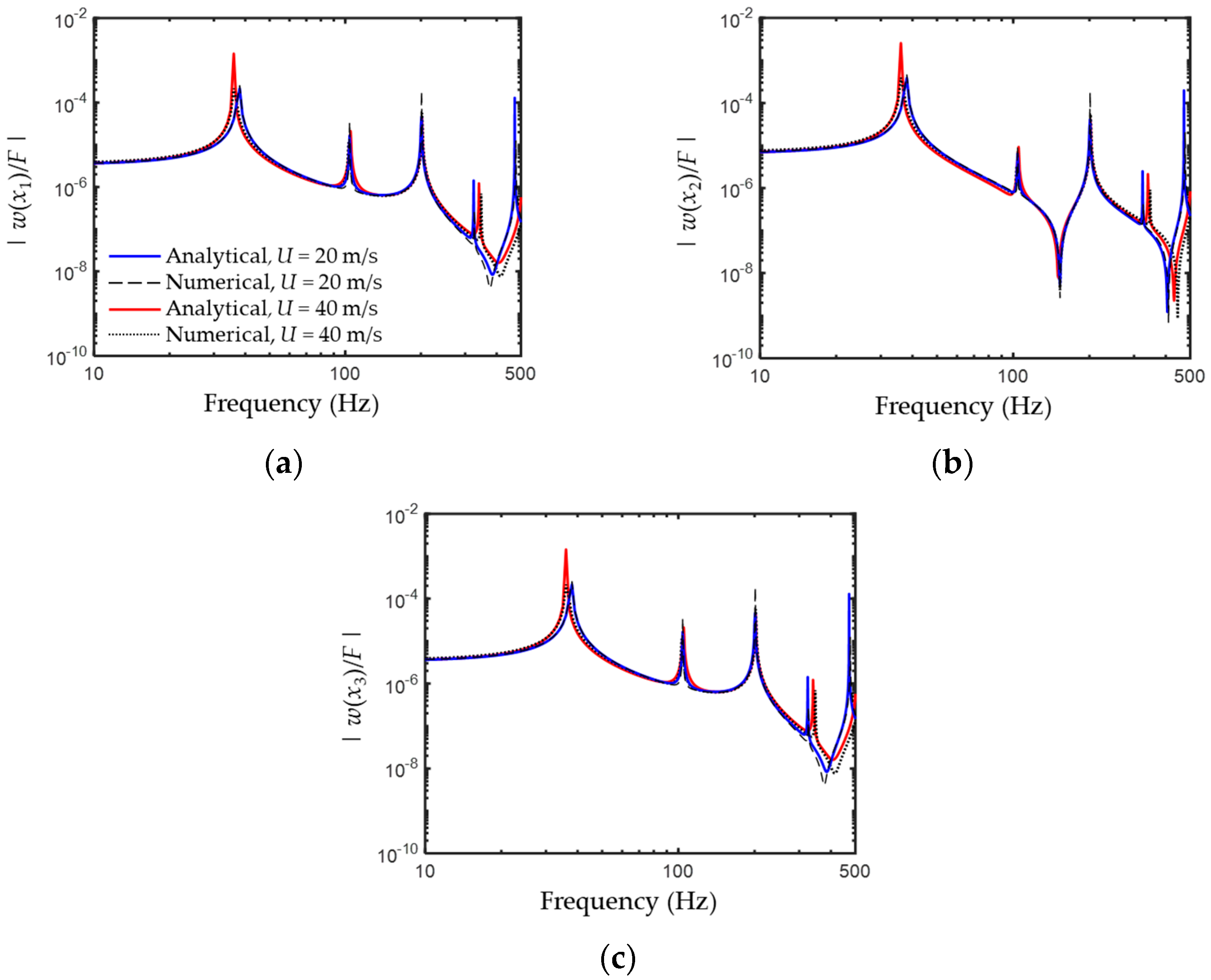
Figure 8 compares the analytical and numerical transfer functions. When the flow velocity was increased, the resonant frequencies of the numerical transfer function shifted toward the low-frequency region. Additionally, the transfer functions at the resonances of the even mode shapes were distinctly predicted, and their magnitudes increased as the flow velocity increased. The numerical transfer function was in good agreement with those of the analytical models.

Figure 9 depicts the predicted flow velocities obtained using Equation (9). The predicted results are corroborated by the input values. The flow velocity also has only minimal measurement error, regardless of resonant frequency. At higher velocities, the transfer function method was more accurate because the magnitude and resonant frequency of the pipe were considerably different from those of the zero-flow velocity pipe. On the other hand, the accuracy of the prediction method at the lower flow velocities dropped at low frequencies. However, when the forced frequency of the excitation sources was higher, the predicted velocities at high frequencies were more accurate because of the inclusion of the transient components of ${\widehat{k}}_{b,2}$, ${\widehat{k}}_{b,3}$, and ${\widehat{k}}_{b,4}$, as shown in Figure 3. Similarly, the measurement accuracies of electromagnetic flowmeters decreased when the flow velocities were lower [24]. Further, the flowrate in the unsteady condition results in measurement errors at low frequencies because of the turbulent intensity [25]. Therefore, to increase the precision of measurement in the transfer function method, the forced frequency of excitation sources must be increased.

5. Conclusions

This study presented a method for predicting the flow velocity of a pipe. The characteristic equation was estimated by analysing the wave propagation of the fluid-conveying pipe. The wavenumbers at low frequencies were complex roots. At a higher excitation frequency, the two wavenumbers converged on two distinct real roots. Using the theoretical wavenumbers and boundary conditions, the harmonic solution of the wave equation was derived, and applied to the transfer function method. A numerical model based on the finite element method was simulated to replace the measured acceleration signals. The finite element equation applied to their interactions was derived using the wave equations of the isotropic solid and fluid. The numerical mode shapes for the flexural vibration of the fluid-conveying pipe were calculated under the force condition at the centre of the pipe. When the flow velocity was increased, the fluid-conveying pipe vibrated asymmetrically and the nodal points of all modes were shifted in the direction of flow because of the increase in the tension force applied on the structure. The numerical transfer functions of the pipe were predicted, and the numerical accuracy was confirmed by comparing the numerical model with the analytical one. The effective flow velocity was predicted using numerical results. At a higher excitation frequency, the accuracy of the prediction method increased because the transient components of the wavenumber at low frequencies influenced the convergence of the numerical solution. Moreover, the error of the predicted flow velocity was minimized at the resonance frequency of the piping system. Finally, the predicted flow velocity precisely converged on the analytical one at a higher flow velocity. For application to actual pipelines, system boundary conditions must be defined because those of complex systems are uncertain. Before measuring the acceleration signals of an actual pipe systems, the boundary conditions must be determined by using blocking mass. The proposed prediction method can be utilized to measure the flow velocity of a real pipe system without installation of flow meters.

References

Fellini, S.; Vesipa, R.; Boano, F.; Ridolfi, L. Fault detection in level and flow rate sensors for safe and performant remote–control in a water supply system. J. Hydroinform.2020, 22, 132–147. [Google Scholar] [CrossRef]
Ghorbani, H.; Wood, D.A.; Choubineh, A.; Tatar, A.; Abarghoyi, P.G.; Madani, M.; Mohamadian, N. Prediction of oil flow rate through an orifice flow meter: Artificial intelligence alternatives compared. Petroleum2020, 6, 404–414. [Google Scholar] [CrossRef]
Han, H.; Jeong, W.; Kim, M. Frequency characteristics of the noise of R600a refrigerant flowing in a pipe with intermittent flow pattern. Int. J. Refrig.2011, 34, 1497–1506. [Google Scholar] [CrossRef]
Lannes, D.P.; Gama, A.L.; Bento, T.F.B. Measurement of flow rate using straight pipes and pipe bends with integrated piezoelectric sensors. Flow Meas. Instrum.2018, 60, 208–216. [Google Scholar] [CrossRef]
Muramatsu, E.; Murakawa, H.; Hashiguchi, D.; Sugimoto, K.; Asano, H.; Wada, S.; Furuichi, N. Applicability of hybrid ultrasonic flow meter for wide–range flow–rate under distorted velocity profile conditions. Exp. Therm. Fluid Sci.2018, 94, 49–58. [Google Scholar] [CrossRef]
Peng, S.; Liao, W.; Tan, H. Performance optimization of ultrasonic flow meter based on computational fluid dynamics. Adv. Mech. Eng.2018, 10, 1–9. [Google Scholar] [CrossRef] [Green Version]
Murakawa, H.; Ichimura, S.; Sugimoto, K.; Asano, H.; Umezawa, S.; Sugita, K. Evaluation method of transit time difference for clamp–on ultrasonic flowmeters in two–phase flows. Exp. Therm. Fluid Sci.2020, 112, 109957. [Google Scholar] [CrossRef]
Nguyen, T.T.; Kikura, H.; Murakawa, H.; Tsuzuki, N. Measurement of bubbly two–phase flow in vertical pipe using multiwave ultrasonic pulsed Doppler method and wire mesh tomography. Energy Procedia2015, 71, 337–351. [Google Scholar] [CrossRef] [Green Version]
Kim, Y.K.; Kim, Y.H. A three accelerometer method for the measurement of flow rate in pipe. J. Acoust. Soc. Am.1996, 100, 717–726. [Google Scholar] [CrossRef]
Kim, Y.B.; Kim, Y.H. A measurement method of the flow rate in a pipe using a microphone array. J. Acoust. Soc. Am.2002, 112, 856–864. [Google Scholar] [CrossRef]
Yang, W.; Park, J. Attenuation of sounds in a pipe with shear flow using layered metamaterials. J. Comput. Acoust.2017, 25, 1750008. [Google Scholar] [CrossRef]
Muggleton, J.M.; Brennan, M.J.; Pinnington, R.J. Wavenumber prediction of waves in buried pipes for water leak detection. J. Sound Vib.2002, 249, 939–954. [Google Scholar] [CrossRef]
Martini, A.; Troncossi, M.; Rivola, A. Automatic leak detection in buried plastic pipes of water supply networks by means of vibration measurements. Shock Vib.2015, 2015, 1–13. [Google Scholar] [CrossRef] [Green Version]
Martini, A.; Rivola, A.; Troncossi, M. Autocorrelation analysis of vibro-acoustic signals measured in a test field for water leak detection. Appl. Sci.2018, 8, 2450. [Google Scholar] [CrossRef] [Green Version]
Butterfield, J.D.; Krynkin, A.; Collins, R.P.; Beck, S.B.M. Experimental investigation into vibro-acoustic emission signal processing techniques to quantify leak flow rate in plastic water distribution pipes. Appl. Acoust.2017, 119, 146–155. [Google Scholar] [CrossRef]
Park, J. Transfer function methods to measure dynamic mechanical properties of complex structures. J. Sound Vib.2005, 288, 57–79. [Google Scholar] [CrossRef]
Park, J.W.; Lee, J.; Park, J. Measurement of viscoelastic properties from the vibration of a compliantly supported beam. J. Acoust. Soc. Am.2011, 130, 3729–3735. [Google Scholar] [CrossRef]
Kim, D.; Hong, S.; Jang, J.; Park, J. Simultaneous determination of position and mass in the cantilever sensor using transfer function method. Appl. Phys. Lett.2013, 103, 033108. [Google Scholar] [CrossRef] [Green Version]
Park, J.W.; Park, B.; Kim, D.; Park, J. Determination of effective mass density and modulus for resonant metamaterials. J. Acoust. Soc. Am.2012, 132, 2793–2799. [Google Scholar] [CrossRef] [Green Version]
Yang, W.; Kim, B.; Cho, S.; Park, J. Experimental method to evaluate effective dynamic properties of a meta–structure for flexural vibrations. Exp. Mech.2017, 57, 417–425. [Google Scholar] [CrossRef]
Blevins, R.D. Flow—Induced Vibration; Van Nostrand Reinhold Co.: New York, NY, USA, 1990. [Google Scholar]
Cook, R.D.; Malkus, D.S.; Plesha, M.E.; Witt, R.J. Concepts and Applications of Finite Element Analysis; John Wiley and Sons: New York, NY, USA, 2007. [Google Scholar]
Simão, M.; Besharat, M.; Carravetta, A.; Ramos, H.M. Flow velocity distribution towards flowmeter accuracy: CFD, UDV, and field tests. Water2018, 10, 1807. [Google Scholar] [CrossRef] [Green Version]
Brunone, B.; Berni, A. Wall shear stress in transient turbulent pipe flow by local velocity measurement. J. Hydraul. Eng.2010, 136, 716–726. [Google Scholar] [CrossRef]
Figure 1.
Alternative method for measurement of flow velocity of pipe by using force excitation and accelerometer signals.
Figure 2.
Analytical model of the flexural vibration of clamped-clamped fluid-conveying pipe with accelerometers attached to the outer surface at different positions.
Figure 3.
Wavenumbers for the fluid-conveying pipe with (a) U = 0 and (b) U = 60 (m/s) at increased excitation frequency.
Figure 4.
Analytical transfer functions for fluid-conveying pipe at (a) x = x1, (b) x2, and (c) x3 with varying flow velocities.
Figure 5.
Analytical mode shapes of the fluid pipe when the flow velocity increased: (a) 1st, (b) 2nd, (c) 3rd, and (d) 4th mode shape.
Figure 6.
Finite element model for the vibration of clamped-clamped fluid-conveying pipe.
Figure 7.
Numerical mode shapes of the fluid-conveying pipe when the flow velocity increased: (a) 1st, (b) 2nd, (c) 3rd, and (d) 4th mode shapes.
Figure 8.
Analytical vs. numerical transfer functions of the fluid-conveying pipes at (a) x = x1, (b) x2, and (c) x3.
Figure 9.
Predicted flow velocities in the fluid pipes.
Publisher’s Note: MDPI stays neutral with regard to jurisdictional claims in published maps and institutional affiliations.