Discrete-Time Position Control for Autonomous Underwater Vehicle under Noisy Conditions

Abstract

This paper deals with the discrete-time position control problem for an autonomous underwater vehicle (AUV) under noisy conditions. Due to underwater noise, the velocity measurements returned by the AUV’s on-board sensors afford low accuracy, downgrading its control quality. Additionally, most of the hydrodynamic parameters of the AUV model are uncertain, further degrading the AUV control accuracy. Based on these findings, a discrete-time control law that improves the position control for the AUV trajectory tracking is presented to reduce the impact of these two factors. The proposed control law extends the Ensemble Kalman Filter and solves the problem of the traditional Ensemble Kalman Filter that underperforms when the hydrodynamic parameters of the AUV model are uncertain. The effectiveness of the proposed discrete-time controller is tested on various simulated scenarios and the results demonstrate that the proposed controller has appealing precision for AUV position tracking under noisy conditions and hydrodynamic parameter uncertainty. The proposed controller outperforms the conventional time-delay controller in root-mean-square error by a percentage range of approximately 72.1–97.4% and requires at least 89.5% less average calculation time than the conventional model predictive control.

1. Introduction

Autonomous underwater vehicles (AUVs) can perform a variety of deep-sea tasks [1]. These tasks broadly involve marine engineering, military, and marine science fields [2,3]. Specifically, tasks such as the inspection of underwater pipelines, enemy target tracking, and marine environmental data collection can be performed by controlling AUVs [4,5]. However, the acquired data quality is highly dependent on the AUV position accuracy [6]. Thus, improving the positional precision of an AUV has recently become a hot research topic. There are two main challenges in achieving an accurate discrete-time position control of an AUV. The first one involves the uncertain hydrodynamic parameters, such as added mass and drag coefficients, and the second, the real-world processing and measurement noise. Due to the uncertainty of system dynamics, common noise filtering algorithms are usually ineffective, and thus the two aforementioned interacting factors impose a low positional accuracy, affecting the precision of AUV control.

Over the past years, the literature has offered quite a few control methods, addressing the hydrodynamic uncertainties of an AUV. The existing AUV control methods can be divided into two major classes: adaptive control and robust control techniques. Adaptive control techniques can automatically compensate for unexpected changes related to the order of the model, parameters, and input signals. It is worth noting that adaptive control compensates, even in the absence of the confines of uncertainties. Nevertheless, the shortcoming of adaptive control is its high energy consumption, as the uncertain hydrodynamic parameters to be adapted impose great computational complexity. Given the limited energy resources of an AUV, this deficiency poses a disadvantage for AUV applications. Despite this, adaptive control is still used with [7] a focuse on proportional integral derivative (PID) controllers for AUV. In this work, the PID control algorithm, despite being classic, is proven to be quite effective for AUV control. Based on a set of saturation functions for trajectory tracking of AUV, Guerrero et al. [8] propose a nonlinear robust PID controller to cope with system uncertainty. In [9], the authors introduce a conventional back-stepping method that applies to AUV platforms for diving control. Sliding mode controllers (SMCs) [10,11] are designed for AUV control in the presence of uncertain hydrodynamics, with their advantage being their implementation simplicity. Based on a sliding mode control, Yan et al. [12] present a robust adaptive SMC. To track the desired path, Xiang et al. [13] propose a robust fuzzy controller for AUV that considers a massive uncertainty of the dynamics. Ref. [14] describes a novel adaptive autopilot, based on ${\mathcal{L}}_1$ adaptive control theory, that is robust to the system uncertainties. To achieve trajectory tracking control, Londhe and Patre [15] propose a robust adaptive tracking controller for AUV.

Compared with adaptive control techniques, robust control techniques require fewer computing resources. However, this type of control demands the knowledge of some of the hydrodynamic parameters, which are usually uncertain. To solve this parameter uncertainty problem, Kumar et al. successively design a continuous time-delay control law [16] and a discrete time-delay control law [17]. Ref. [18] presents an enhanced time-delay controller (TDC) for the position control of AUV. The enhanced TDC is computationally simple and robust to unmodeled dynamics and disturbances. These time-delay controllers (TDCs) are designed by employing the time-delay estimator (TDE) that is capable of estimating uncertain hydrodynamic parameters, using time-delayed state derivatives and control inputs [19,20]. The TDCs have two additional advantages, namely, saving computing resources, and having no requirements of prior information about uncertain parameters. However, it should be mentioned that all aforementioned controllers [7,8,9,10,11,12,13,14,15,16,17,18] do not consider any process and measurement noises.

Given that the Global Positioning System (GPS) navigation system does not operate underwater, AUVs estimate their position utilizing acoustic and optical devices that are usually considered to be on-board navigation sensors [21,22]. Both these sensor types feed the positional AUV controller with velocity information from which the traveled distance is derived. However, especially in the deep-sea, sensor measurements are inevitably affected by noise, influencing the quality of the measurement data and ultimately limiting the precision of the AUV controller. Moreover, the mathematical model of AUV imposes some process noise. Thus, the process and measurement noises incommode the design of a motion AUV controller. To deal with these noises, several estimation approaches have been made. Ermayanti et al. [23] present a Fuzzy Kalman Filter (FKF) to estimate the AUV position, while [24] propose an Ensemble Kalman Filter (EnKF). Compared with FKF, EnKF manages a more accurate position estimation, and additionally, the computational complexity of EnKF is less than that of FKF, saving energy for the AUV platforms evaluated here. Fan et al. [25] introduce a comprehensive scheme that combines a Kalman filter-type navigation for both the cross-track and heading control of AUV. However, current estimation methods become invalid if any uncertain hydrodynamic parameters exist. Yan et al. [26] utilize an advanced control strategy, i.e., the model predictive control (MPC), to improve the trajectory tracking stability of an AUV under external disturbances and noise. Yang et al. [27] propose a high aiming precision method for the unmanned combat air vehicle (UCAV) under the MPC framework. These MPC algorithms can bring a satisfactory control precision. However, exploiting MPC imposes a sizable computational complexity and energy consumption during the mission. In [28], the deterministic artificial intelligence (D.A.I.) is used to eliminate the motion trajectory tracking error for unmanned underwater vehicles in continuous time. However, the performance of D.A.I. is severely degraded by the discretization implementation [29].

In practice, AUV is commonly driven by a propulsion system and controlled by an on-board computer. Given that the computer only processes discrete digital signals, the goal is to design a discrete-time controller. Hence, in this work, the discrete-time position control for AUV under noisy conditions is studied and a discrete-time control law for trajectory tracking is proposed. The contributions of this paper are as follows:

• A control law, which is a modified algorithm based on the EnKF that first introduces the TDE into the EnKF.
• An AUV positional control method that solves the problem of uncertainty in the hydrodynamics parameters, where the traditional EnKF underperforms.
• Since the proposed solution utilizes the TDE algorithm, it does not need any information about the bounds of uncertain terms of the system hydrodynamics, except the rigid body inertia matrix parameter.
• Several Matlab/Simulink simulations are performed and the result demonstrates that the proposed discrete-time control law attains better position control precision, compared to the existing control laws, for trajectory tracking. The scenarios include various noise conditions, where the precision of the proposed control law in trajectory tracking is verified and the presented technique is also tested on several sampling times or ensembles. Finally, under the same noise conditions, the performance of the proposed discrete-time control law is tested against that of the conventional linear controller, TDC, and MPC controller.

The rest of this paper is organized into four parts as follows. Section 2 introduces the AUV model architecture, while in Section 3 a stability analysis of the proposed discrete-time controller is presented. Additionally, the steps to implement the proposed modified EnKF algorithm are expressed. Finally, Section 4 presents the simulation results, and Section 5 concludes this work.

2. System Model Building

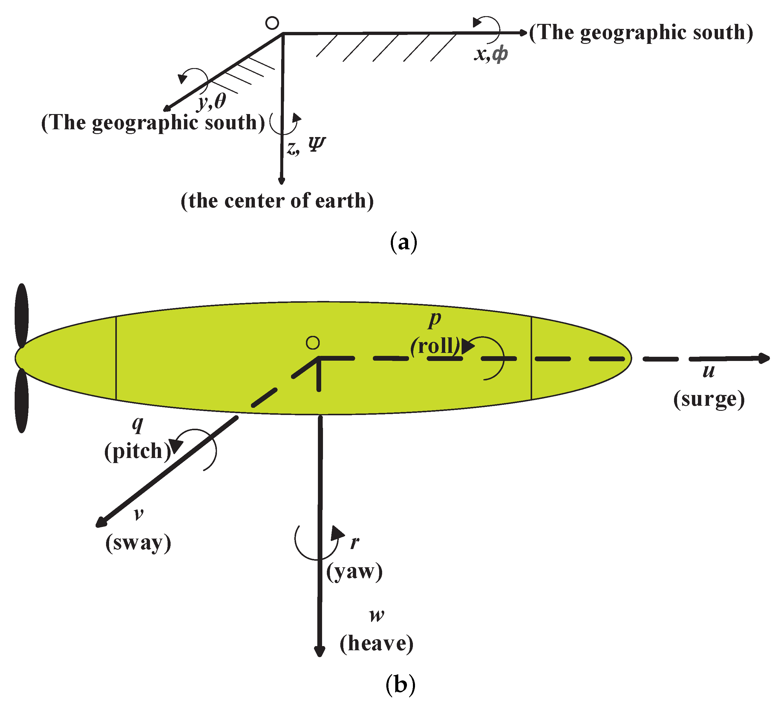
To describe the motion of the AUV in three-dimensional (3D) space, two coordinate systems are usually required (Figure 1). The first one involves the earth-fixed frame $\left\{E\right\}$, while the other one is the body-fixed frame $\left\{B\right\}$. Specifically, in Figure 1a, the position and orientation of the AUV can be defined by the earth-fixed frame, while in Figure 1b, the body-fixed frame as a moving coordinate system describes the AUV velocity and acceleration. Since an AUV motion involves of six degrees of freedom (6-DoF), its dynamics can be written as follows [30]:

$$\begin{array}{cc}\hfill & \mathit{M}\dot{\mathit{v}}+\mathit{C}\left(\mathit{v}\right)\mathit{v}+\mathit{D}\left(\mathit{v}\right)\mathit{v}+\mathit{g}\left(\mathit{\eta }\right)=\mathit{\tau }\hfill \end{array}$$

(1)

Reference [30] also describes the the kinematics of AUV as:

$$\begin{array}{c}\hfill \dot{\mathit{\eta }}=\mathit{J}\left(\mathit{\eta }\right)\mathit{v}\end{array}$$

(2)

In Equation (1), $\mathit{M}={\mathit{M}}_{\mathit{RB}}+{\mathit{M}}_{\mathit{A}}$, where $\mathit{M}$ represents the inertia matrix, and ${\mathit{M}}_{\mathit{RB}}$ and ${\mathit{M}}_{\mathit{A}}$ denote the rigid body mass matrix and the added mass matrix, respectively. $\mathit{C}\left(\mathit{v}\right)$ denotes the Coriolis and the centripetal matrix of the rigid body $\left({\mathit{C}}_{\mathit{RB}}\right)$ with added mass $\left({\mathit{C}}_{\mathit{A}}\right)$. Therefore, $\mathit{C}\left(\mathit{v}\right)={\mathit{C}}_{\mathit{RB}}\left(\mathit{v}\right)+{\mathit{C}}_{\mathit{A}}\left(\mathit{v}\right)$. $\mathit{D}\left(\mathit{v}\right)$ represents the matrix, including the linear and the quadratic drag. Vector $\mathit{g}\left(\mathit{\eta }\right)$ denotes the restoring force and moment. $\mathit{v}={\left[uvwpqr\right]}^T$, ${\left[uvw\right]}^T$ are the linear velocities and ${\left[pqr\right]}^T$ are the angular velocities. $\mathit{\tau }$ represents the control input, which includes the forces and moments. In Equation (2), $\mathit{\eta }={\left[xyz\varphi \theta \psi \right]}^T$. Considering frame $\left\{E\right\}$, x, y, and z describe the position of AUV for surge, sway, and heave, respectively. Likewise, $\varphi$, $\theta$, and $\psi$ represent the Euler angles for roll, pith and yaw, respectively. The non-singular $\mathit{J}\left(\mathit{\eta }\right)$ denotes the kinematic transformation matrix from the frame $\left\{B\right\}$ to frame $\left\{E\right\}$.

In this paper, the following assumptions are made, considering the study of the discrete-time position control for AUV:

• The AUV is regarded as a rigid body.
• The vehicle is symmetric, and thus ${\mathit{M}}_{\mathit{RB}}$ and ${\mathit{M}}_{\mathit{A}}$ are positive definite.
• During the controller design, all AUV model parameters are unknown, except from ${\mathit{M}}_{\mathit{RB}}$.
• Given that most AUVs are designed with pitch and roll stability, in the model, the pitch and roll motion are neglected.
• The motions of surge, sway, and heave are considered and studied. Given that $r\left(t\right)$ ≃ 0 and $\psi \left(t\right)$ ≃ ${\psi }_c$, with $|{\psi }_c|<\pi /2$.

By neglecting the pitch and roll motions, the AUV model can be simplified and degraded from a 6-DoF problem to a 4-DoF. Thus, the resulting 4-DoF of hydrodynamic and kinematic equations is used [31]:

$$\begin{array}{cc}\hfill & \mathit{M}=\left[\begin{array}{cccc}{m}_u& 0& 0& 0\\ 0& m_v& 0& 0\\ 0& 0& m_w& 0\\ 0& 0& 0& I_r\end{array}\right]\hfill \end{array}$$

(3)

$$\begin{array}{cc}\hfill & \mathit{C}\left(\mathit{v}\left(t\right)\right)=\left[\begin{array}{cccc}0& 0& 0& -m_{u}v\left(t\right)\\ 0& 0& 0& m_{v}u\left(t\right)\\ 0& 0& 0& 0\\ m_{u}v\left(t\right)& -m_{v}u\left(t\right)& 0& I_r\end{array}\right]\hfill \end{array}$$

(4)

$$\begin{array}{cc}\mathit{D}\left(\mathit{v}\left(t\right)\right)=\left[\begin{array}{cc}{k}_u+k_{u\left|u\right|}\left|u\left(t\right)\right|& 0\\ 0& k_v+k_{v\left|v\right|}\left|v\left(t\right)\right|\\ 0& 0\\ 0& 0\end{array}\right.\hfill & \\ & \hfill \left.\begin{array}{cc}0& 0\\ 0& 0\\ k_w+k_{w\left|w\right|}\left|w\left(t\right)\right|& 0\\ 0& k_r+k_{r\left|r\right|}\left|r\left(t\right)\right|\end{array}\right]\end{array}$$

(5)

$$\begin{array}{cc}\hfill & \mathit{g}\left(\mathit{\eta }\left(t\right)\right)={[00-W\left(t\right)0]}^T\hfill \end{array}$$

(6)

$$\begin{array}{cc}\hfill & \mathit{\tau }\left(t\right)=\left[F_u\left(t\right)F_v\left(t\right)F_w\left(t\right)T_r\left(t\right)\right]\hfill \end{array}$$

(7)

$$\begin{array}{cc}\hfill & \mathit{J}\left(\mathit{\eta }\left(t\right)\right)=\left[\begin{array}{cccc}cos\left({\psi }_c\right)& -sin\left({\psi }_c\right)& 0& 0\\ sin\left({\psi }_c\right)& cos\left({\psi }_c\right)& 0& 0\\ 0& 0& 1& 0\\ 0& 0& 0& 1\end{array}\right]\hfill \end{array}$$

(8)

3. Discrete-Time Controller Design in Trajectory Tracking

In this section, the design of the proposed discrete-time controller for AUV positional control in trajectory tracking noisy conditions is presented.

The control objective is to design a discrete-time control law, where the AUV can follow the reference trajectory as the time increases. The schematic diagram of the proposed controller is shown in Figure 2. The symbols used throughout this paper are presented in

Table 1. The nomenclature.

Symbol	Description	Unit
T	The sampling time	s
$\mathit{\eta }\left(k\right)$	The real position at time $kT$	m
${\mathit{\eta }}_r\left(k\right)$	The reference position at time $kT$	m
$\widehat{\mathit{\eta }}\left(k\right)$	The estimated position generated by proposed modified algorithm at time $kT$	m
${\tilde{\mathit{\eta }}}^e\left(k\right)$	The estimated position error at time $kT$, ${\tilde{\mathit{\eta }}}^e\left(k\right)={\mathit{\eta }}_r\left(k\right)-\widehat{\mathit{\eta }}\left(k\right)$	m
$\tilde{\mathit{\eta }}\left(k\right)$	The position error at time $kT$, $\tilde{\mathit{\eta }}\left(k\right)={\mathit{\eta }}_r\left(k\right)-\mathit{\eta }\left(k\right)$	m
$\mathit{v}\left(k\right)$	The real velocity at time $kT$	$m/s$
${\mathit{v}}_r\left(k\right)$	The reference velocity at time $kT$	$m/s$
$\widehat{\mathit{v}}\left(k\right)$	The estimated velocity generated by proposed modified algorithm at time $kT$	$m/s$
${\tilde{\mathit{v}}}^e\left(k\right)$	The estimated velocity error at time $kT$, ${\tilde{\mathit{v}}}^e\left(k\right)={\mathit{v}}_r\left(k\right)-\widehat{\mathit{v}}\left(k\right)$	$m/s$
$\tilde{\mathit{v}}\left(k\right)$	The velocity error at time $kT$, $\tilde{\mathit{v}}\left(k\right)={\mathit{v}}_r\left(k\right)-\mathit{v}\left(k\right)$	$m/s$

.

3.1. Discrete-Time Control Law

For a continuous system, as a rule, there are two methods to design a discrete-time controller, either by discretizing an analog controller, or by building a discrete-time model of a continuous system and subsequently deriving the discrete-time controller. The difference between these two methods is that the first one uses the derivative of the system state in the control law. However, the system state is obtained through sensors that are affected by the noise, and thus, if the control law contains the derivative of the state of the system, it will increase the influence of the noise factor. Therefore, the second method is adopted in this work.

Hence, Equation (1) can be rewritten as follows:

$$\begin{array}{cc}\hfill & {\mathit{M}}_{\mathit{RB}}\dot{\mathit{v}}+{\mathit{M}}_{\mathit{A}}\dot{\mathit{v}}+\mathit{C}\left(\mathit{v}\right)\mathit{v}+\mathit{D}\left(\mathit{v}\right)\mathit{v}+\mathit{g}\left(\mathit{\eta }\right)=\mathit{\tau }\hfill \end{array}$$

(9)

let $\mathit{f}\left(t\right)=\mathit{C}\left(\mathit{v}\right)\mathit{v}+\mathit{D}\left(\mathit{v}\right)\mathit{v}+\mathit{g}\left(\mathit{\eta }\right)$, and one can obtain:

$$\begin{array}{cc}\hfill & {\mathit{M}}_{\mathit{RB}}\dot{\mathit{v}}\left(t\right)+{\mathit{M}}_{\mathit{A}}\dot{\mathit{v}}\left(t\right)+\mathit{f}\left(t\right)=\mathit{\tau }\left(t\right)\hfill \end{array}$$

(10)

In Equation (10), $\mathit{f}\left(t\right)$ and ${\mathit{M}}_{\mathit{A}}$ are assumed to be unknown. In other words, only the parameter ${\mathit{M}}_{\mathit{RB}}$ is known.

For the sampling time T, the control input generated from the discrete-time controller is considered to be constant during the sample interval, on account of zero-order holder (see Figure 2). Thus, the control input $\mathit{\tau }\left(t\right)$ remains constant $\mathit{\tau }\left(k\right)$ from time $kT$ to time $(k+1)T$. The relationship between the control input and the consequent velocity is presented in Figure 3.

By integrating Equation (10) concerning the time over the sample interval,

$$\begin{array}{cc}\hfill & {\mathit{M}}_{\mathit{RB}}(\mathit{v}(k+1)-\mathit{v}\left(k\right))+\mathit{H}\left(k\right)=T\mathit{\tau }\left(k\right)\hfill \end{array}$$

(11)

where

$$\begin{array}{cc}\hfill & \mathit{H}\left(k\right)={\mathit{M}}_{\mathit{A}}(\mathit{v}(k+1)-\mathit{v}\left(k\right))+{\int }_{kT}^{kT+T}\mathit{f}\left(\xi \right)d\xi \hfill \end{array}$$

(12)

with $\mathit{H}\left(k\right)$ representing the entire uncertainty of the AUV hydrodynamics. According to [17], Equation (11) is considered to be an accurate discrete-time model of the continuous system of Equation (10). From Equation (11), one can write the following:

$$\begin{array}{cc}\hfill & \mathit{v}(k+1)={\mathit{M}}_{\mathit{RB}}^{-\mathbf{1}}(T\mathit{\tau }\left(k\right)-\mathit{H}\left(k\right))+\mathit{v}\left(k\right)\hfill \end{array}$$

(13)

The control law is given as follows:

$$\begin{array}{cc}\hfill & \mathit{\tau }\left(k\right)=T^{-1}({\mathit{M}}_{\mathit{RB}}(\mathit{u}\left(k\right)-\widehat{\mathit{v}}\left(k\right))+\widehat{\mathit{H}}\left(k\right))\hfill \end{array}$$

(14)

where

$$\begin{array}{cc}\hfill & \mathit{u}\left(k\right)={\mathit{J}}^{-1}({\dot{\mathit{\eta }}}_r(k+1)+{\mathit{K}}_{\mathit{P}}{\tilde{\mathit{\eta }}}^e\left(k\right)+{\mathit{K}}_{\mathit{D}}{\dot{\tilde{\mathit{\eta }}}}^e\left(k\right))\hfill \end{array}$$

(15)

with ${\mathit{K}}_{\mathit{P}}$ and ${\mathit{K}}_{\mathit{D}}$ being the proportional gain matrix and the derivative gain matrix, respectively.

In Equation (14), $\widehat{\mathit{H}}\left(k\right)$ denotes an estimate of $\mathit{H}\left(k\right)$ by TDE. Hence, $\widehat{\mathit{H}}\left(k\right)$ can be expressed as follows:

$$\begin{array}{cc}\hfill & \widehat{\mathit{H}}\left(k\right)=\mathit{H}(k-1)\hfill \end{array}$$

(16)

From Equation (11), one can write the following:

$$\begin{array}{cc}\hfill \mathit{H}(k-1)& =T\mathit{\tau }(k-1)-{\mathit{M}}_{\mathit{RB}}(\mathit{v}\left(k\right)-\mathit{v}(k-1))\hfill \\ & =\widehat{\mathit{H}}\left(k\right)\hfill \end{array}$$

(17)

Because $\mathit{v}\left(k\right)$ and $\mathit{v}(k-1)$ in Equation (17) are not available, they can be replaced by the estimate $\widehat{\mathit{v}}\left(k\right)$ and $\widehat{\mathit{v}}(k-1)$. Finally, by substituting $\widehat{\mathit{H}}\left(k\right)$ into Equation (14), the summative control law is obtained:

$$\begin{array}{cc}\hfill & \mathit{\tau }\left(k\right)=T^{-1}{\mathit{M}}_{\mathit{RB}}(\mathit{u}\left(k\right)-2\widehat{\mathit{v}}\left(k\right)+\widehat{\mathit{v}}(k-1))+\mathit{\tau }(k-1)\hfill \end{array}$$

(18)

3.2. Stability Analysis

By combining Equation (11) with Equation (14),

$$\begin{array}{cc}\hfill & \mathit{H}\left(k\right)-\widehat{\mathit{H}}\left(k\right)={\mathit{M}}_{\mathit{RB}}(\mathit{u}\left(k\right)-\widehat{\mathit{v}}\left(k\right)-\mathit{v}(k+1)+\mathit{v}\left(k\right))\hfill \end{array}$$

(19)

$\mathit{u}\left(k\right)$ is substituted into Equation (19) and one can obtain the following:

$$\begin{array}{cc}\hfill {\mathit{M}{}_{\mathit{RB}}}^{-1}(\mathit{H}\left(k\right)-\widehat{\mathit{H}}\left(k\right))=& {\mathit{J}}^{-1}({\dot{\mathit{\eta }}}_r(k+1)+{\mathit{K}}_{\mathit{P}}{\tilde{\mathit{\eta }}}^e\left(k\right)+{\mathit{K}}_{\mathit{D}}{\dot{\tilde{\mathit{\eta }}}}^e\left(k\right))\hfill \\ & -\mathit{v}(k+1)+\mathit{v}\left(k\right)-\widehat{\mathit{v}}\left(k\right)\hfill \end{array}$$

(20)

One can write from Equation (2) the following:

$$\begin{array}{c}\hfill \left\{\begin{array}{c}\mathit{v}(k+1)={\mathit{J}}^{-1}\dot{\mathit{\eta }}(k+1)\hfill \\ \mathit{v}\left(k\right)={\mathit{J}}^{-1}\dot{\mathit{\eta }}\left(k\right)\hfill \\ \widehat{\mathit{v}}\left(k\right)={\mathit{J}}^{-1}\dot{\widehat{\mathit{\eta }}}\left(k\right)\hfill \end{array}\right.\end{array}$$

(21)

Combining Equation (20) with Equation (21) yields the following:

$$\begin{array}{cc}\hfill & {\mathit{J}}^{-1}({\dot{\mathit{\eta }}}_r(k+1)-\dot{\mathit{\eta }}(k+1)+{\mathit{K}}_{\mathit{P}}{\tilde{\mathit{\eta }}}^e\left(k\right)+{\mathit{K}}_{\mathit{D}}{\dot{\tilde{\mathit{\eta }}}}^e\left(k\right))\hfill \\ & ={\mathit{M}{}_{\mathit{RB}}}^{-1}(\mathit{H}\left(k\right)-\widehat{\mathit{H}}\left(k\right))+{\mathit{J}}^{-1}(\dot{\mathit{\eta }}\left(k\right)-\dot{\widehat{\mathit{\eta }}}\left(k\right))\hfill \end{array}$$

(22)

Let $\mathit{e}\left(k\right)=\widehat{\mathit{\eta }}\left(k\right)-\mathit{\eta }\left(k\right)$. It is assumed that $\mathit{e}\left(k\right)$ and $\dot{\mathit{e}}\left(k\right)$ are all bounded. One can write the following:

$$\begin{array}{c}\hfill {\tilde{\mathit{\eta }}}^e\left(k\right)={\mathit{\eta }}_r\left(k\right)-\widehat{\mathit{\eta }}\left(k\right)=\widehat{\mathit{\eta }}\left(k\right)-\mathit{e}\left(k\right)\end{array}$$

(23)

From Equations (22) and (23) one can write the following:

$$\begin{array}{cc}\hfill & {\mathit{J}}^{-1}(\dot{\widehat{\mathit{\eta }}}(k+1)+{\mathit{K}}_{\mathit{P}}(\widehat{\mathit{\eta }}\left(k\right)-\mathit{e}\left(k\right))+{\mathit{K}}_{\mathit{D}}(\dot{\widehat{\mathit{\eta }}}\left(k\right)-\dot{\mathit{e}}\left(k\right)))\hfill \\ & ={\mathit{M}{}_{\mathit{RB}}}^{-1}(\mathit{H}\left(k\right)-\widehat{\mathit{H}}\left(k\right))-{\mathit{J}}^{-1}\dot{\mathit{e}}\left(k\right)\hfill \end{array}$$

(24)

Equation (24) can be rewritten as follows:

$$\begin{array}{cc}\hfill & \dot{\widehat{\mathit{\eta }}}(k+1)+{\mathit{K}}_{\mathit{P}}\widehat{\mathit{\eta }}\left(k\right)+{\mathit{K}}_{\mathit{D}}\dot{\widehat{\mathit{\eta }}}\left(k\right)=\mathit{J}{\mathit{M}{}_{\mathit{RB}}}^{-1}(\mathit{H}\left(k\right)-\widehat{\mathit{H}}\left(k\right))\hfill \\ \hfill & +{\mathit{K}}_{\mathit{P}}\mathit{e}\left(k\right)+{\mathit{K}}_{\mathit{D}}\dot{\mathit{e}}\left(k\right)+\dot{\mathit{e}}\left(k\right)\hfill \end{array}$$

(25)

$\mathit{\epsilon }\left(k\right)$ is defined as follows:

$$\begin{array}{c}\hfill \mathit{\epsilon }\left(k\right)={{\mathit{M}}_{\mathit{RB}}}^{-1}(\widehat{\mathit{H}}\left(k\right)-\mathit{H}\left(k\right))\end{array}$$

(26)

Equation (26) shows that $\mathit{\epsilon }\left(k\right)$ can be considered to represent the approximate error in the estimate $\widehat{\mathit{H}}\left(k\right)$ by TDE.

Equation (25) can be simplified by using the forward difference approximation. The simplified equation becomes the following:

$$\begin{array}{cc}\hfill & \widehat{\mathit{\eta }}(k+2)+({\mathit{K}}_{\mathit{D}}-\mathit{I})\widehat{\mathit{\eta }}(k+1)+({\mathit{K}}_{\mathit{P}}-{\mathit{K}}_{\mathit{D}})\widehat{\mathit{\eta }}\left(k\right)\hfill \\ \hfill & =-\mathit{TJ}\mathit{\epsilon }\left(t\right)+{\mathit{K}}_{\mathit{P}}\mathit{e}\left(k\right)+({\mathit{K}}_{\mathit{D}}+\mathit{I})\dot{\mathit{e}}\left(k\right)\hfill \end{array}$$

(27)

If $\left(-\mathit{TJ}\mathit{\epsilon }\left(k\right)+{\mathit{K}}_{\mathit{P}}\mathit{e}\left(k\right)+({\mathit{K}}_{\mathit{D}}+\mathit{I})\dot{\mathit{e}}\left(k\right)\right)$ is bounded, then the Bounded Input Bounded Output (BIBO) stability of the presented control law can be proved. Here, ${\mathit{K}}_{\mathit{P}}\mathit{e}\left(k\right)+({\mathit{K}}_{\mathit{D}}+\mathit{I})\dot{\mathit{e}}\left(k\right)$ is bounded and the boundedness of $\mathit{\epsilon }\left(k\right)$ will be shown as follows.

From Equations (11), (14) and (26) one can write the following:

$$\begin{array}{c}\hfill \mathit{\epsilon }\left(k\right)=\mathit{v}(k+1)-\mathit{u}\left(k\right)-\mathit{v}\left(k\right)+\widehat{\mathit{v}}\left(k\right)\end{array}$$

(28)

let ${\mathit{H}}_1\left(k\right)={\int }_{kT}^{kT+T}\mathit{f}\left(\xi \right)d\xi$ and one can obtain:

$$\begin{array}{c}\hfill \mathit{H}\left(k\right)={\mathit{H}}_1\left(k\right)+{\mathit{M}}_{\mathit{A}}(\mathit{v}(k+1)-\mathit{v}\left(k\right))\end{array}$$

(29)

By using Equations (11) and (29) one can write the following:

$$\begin{array}{c}\hfill \mathit{M}(\mathit{v}(k+1)-\mathit{v}\left(k\right))+{\mathit{H}}_1\left(k\right)=T\mathit{\tau }\left(k\right)\end{array}$$

(30)

From Equation (28) one can write the following:

$$\begin{array}{cc}\hfill \mathit{M}\mathit{\epsilon }\left(k\right)& =\mathit{M}\mathit{v}(k+1)-\mathit{M}\mathit{u}\left(k\right)-\mathit{M}\mathit{v}\left(k\right)+\mathit{M}\widehat{\mathit{v}}\left(k\right)\hfill \\ \hfill & =T\mathit{\tau }\left(k\right)-{\mathit{H}}_1\left(k\right)-\mathit{M}\mathit{u}\left(k\right)+\mathit{M}\widehat{\mathit{v}}\left(k\right)\hfill \end{array}$$

(31)

Substituting $\mathit{\tau }\left(k\right)$ into the above equation, we get the following:

$$\begin{array}{cc}\hfill \mathit{M}\mathit{\epsilon }\left(k\right)=& ({\mathit{M}}_{\mathit{RB}}-\mathit{M})\mathit{u}\left(k\right)+(\mathit{M}-{\mathit{M}}_{\mathit{RB}})\widehat{\mathit{v}}\left(k\right)\hfill \\ \hfill & +\widehat{\mathit{H}}\left(k\right)-{\mathit{H}}_1\left(k\right)\hfill \end{array}$$

(32)

Substituting $\widehat{\mathit{H}}\left(k\right)$ into Equation (32), we get the following:

$$\begin{array}{cc}\hfill \mathit{M}\mathit{\epsilon }\left(k\right)=& ({\mathit{M}}_{\mathit{RB}}-\mathit{M})\mathit{u}\left(k\right)+(\mathit{M}-{\mathit{M}}_{\mathit{RB}})\widehat{\mathit{v}}\left(k\right)\hfill \\ \hfill & +T\mathit{\tau }(k-1)-{\mathit{M}}_{\mathit{RB}}(\mathit{v}\left(k\right)-\mathit{v}(k-1))-{\mathit{H}}_1\left(k\right)\hfill \end{array}$$

(33)

Using Equation (30) one can write the following:

$$\begin{array}{c}\hfill T\mathit{\tau }(k-1)=\mathit{M}(\mathit{v}\left(k\right)-\mathit{v}(k-1))+{\mathit{H}}_1(k-1)\end{array}$$

(34)

Substituting Equation (34) into Equation (33), we get the following:

$$\begin{array}{cc}\hfill \mathit{M}\mathit{\epsilon }\left(k\right)=& -{\mathit{M}}_{\mathit{A}}\mathit{u}\left(k\right)+{\mathit{M}}_{\mathit{A}}\widehat{\mathit{v}}\left(k\right)\hfill \\ \hfill & +{\mathit{M}}_{\mathit{A}}(\mathit{v}\left(k\right)-\mathit{v}(k-1))+{\mathit{H}}_1(k-1)-{\mathit{H}}_1\left(k\right)\hfill \end{array}$$

(35)

From Equation (28), one can obtain the following:

$$\begin{array}{c}\hfill \mathit{v}\left(k\right)-\mathit{v}(k-1)=\mathit{\epsilon }(k-1)+\mathit{u}(k-1)-\widehat{\mathit{v}}(k-1)\end{array}$$

(36)

Substituting Equation (36) into Equation (35), we get the following:

$$\begin{array}{c}\hfill \mathit{\epsilon }\left(k\right)=\mathit{A}\mathit{\epsilon }(k-1)+{\mathit{B}}_{\mathbf{1}}+{\mathit{B}}_{\mathbf{2}}\end{array}$$

(37)

where

$$\begin{array}{c}\hfill \mathit{A}={\mathit{M}}^{-1}{\mathit{M}}_{\mathit{A}}\end{array}$$

(38)

$$\begin{array}{c}\hfill {\mathit{B}}_{\mathbf{1}}={\mathit{M}}^{-1}{\mathit{M}}_{\mathit{A}}(\mathit{u}(k-1)-\mathit{u}\left(k\right)+\widehat{\mathit{v}}\left(k\right)-\widehat{\mathit{v}}(k-1))\end{array}$$

(39)

$$\begin{array}{c}\hfill {\mathit{B}}_{\mathbf{2}}={\mathit{M}}^{-1}({\mathit{H}}_1(k-1)-{\mathit{H}}_1\left(k\right))\end{array}$$

(40)

Here, ${\mathit{B}}_{\mathbf{1}}$ and ${\mathit{B}}_{\mathbf{1}}$ are considered to be the bounded disturbance. According to [17], it is already proven that the eigenvalues of $\mathit{A}$ lie within the unit disc. Therefore, $\mathit{\epsilon }\left(k\right)$ is bounded and the BIBO stability of the presented control law is proved.

3.3. The Modified Algorithm Based on EnKF

This subsection introduces the proposed algorithm, relying on a modified EnKF, which involves a TDE scheme canceling the uncertain terms of the state space form. It should be noted that the proposed strategy combining the EnKF with TDE offers overall robustness against large noise levels and great system parameter uncertainties. TDE is used, as it requires only the ${\mathit{M}}_{\mathit{RB}}$ parameter to be known. This is important, as the remaining parameters, such as $\mathit{C}\left(\mathit{v}\right)$, $\mathit{D}\left(\mathit{v}\right)$, and $\mathit{g}\left(\mathit{\eta }\right)$, are usually unknown in practical applications; thus, exploiting TDE the proposed method affords broadening the uncertainty bounds of the involved parameters. The motivations for using the EnKF over the Extended Kalman Filter (EKF) counterpart are that the EnKF is a Kalman Filter variant appropriate for large scale-problems as the one investigated in this paper, and is more accurate and efficient than EKF, even for relatively low ensembles, i.e., N > 50 [32,33,34].

According to the separation principle, the optimal control and state estimation problems can be decoupled in some situations. Given that the process and the observation noise are Gaussian, the optimal solution can be separated into a Kalman Filter and a linear quadratic regulator, known as linear–quadratic Gaussian control. In this work, EnKF is a linear variant of the Kalman Filter, and thus, TDE can be considered to be a linear estimation (or optimal control) [35]. Therefore, the separation principle is still available for the designed controller.

Hence, for the proposed controller, the state space form becomes the following:

$$\begin{array}{cc}\hfill \mathit{v}\left(k\right)=& \mathit{v}(k-1)+{\mathit{M}}_{\mathit{RB}}^{-\mathbf{1}}(\widehat{\mathit{H}}(k-1)-\mathit{H}(k-1))-\widehat{\mathit{v}}(k-1)\hfill \\ \hfill & +{\mathit{J}}^{-1}({\dot{\mathit{\eta }}}_r\left(k\right)+{\mathit{K}}_{\mathit{P}}{\tilde{\mathit{\eta }}}^e(k-1)+{\mathit{K}}_{\mathit{D}}{\dot{\tilde{\mathit{\eta }}}}^e(k-1))\hfill \end{array}$$

(41)

where $\mathit{H}\left(k\right)$ contains all the uncertain terms. The process noise is not contained in Equation (41), and therefore, the uncorrelated process noise $\mathit{\varsigma }\left(k\right)$ and the measurement noise $\mathit{\zeta }\left(k\right)$ are added into the Equation (41):

$$\begin{array}{cc}\hfill \mathit{v}\left(k\right)=& \mathit{v}(k-1)+{\mathit{M}}_{\mathit{RB}}^{-\mathbf{1}}(\widehat{\mathit{H}}(k-1)-\mathit{H}(k-1))-\widehat{\mathit{v}}(k-1)\hfill \\ \hfill & +{\mathit{J}}^{-1}({\dot{\mathit{\eta }}}_r\left(k\right)+{\mathit{K}}_{\mathit{P}}{\tilde{\mathit{\eta }}}^e(k-1)+{\mathit{K}}_{\mathit{D}}{\dot{\tilde{\mathit{\eta }}}}^e(k-1))\hfill \\ \hfill & +\mathit{\varsigma }(k-1)\hfill \end{array}$$

(42)

The observation equation is as follows:

$$\begin{array}{cc}\hfill & \mathit{Z}\left(k\right)={\mathit{H}}_{\mathit{o}}\mathit{v}\left(k\right)+\mathit{\zeta }\left(k\right)\hfill \end{array}$$

(43)

where ${\mathit{H}}_{\mathit{o}}$ is the observation operator. The $\mathit{\varsigma }\left(k\right)$ and $\mathit{\zeta }\left(k\right)$ are random Gaussian noise with mean 0. Their covariance matrix is $\mathit{Q}$ and $\mathit{R}$, respectively.

The modified algorithm based on the EnKF [24] becomes the following:

• Setting the initial estimated velocity $\widehat{\mathit{v}}\left(0\right)=0$.
• By using the state space form, the N-ensemble for variable state is presented as follows:

  $$\begin{array}{cc}\hfill {\widehat{\mathit{v}}}_i^{-}\left(k\right)=& \widehat{\mathit{v}}(k-1)+\left({\mathit{M}}_{RB}^{-1}(\widehat{\mathit{H}}(k-1)-\mathit{H}(k-1))\right)\hfill \\ \hfill & +{\mathit{J}}^{-1}({\dot{\mathit{\eta }}}_r\left(k\right)+{\mathit{K}}_{\mathit{P}}{\tilde{\mathit{\eta }}}^e(k-1)+{\mathit{K}}_{\mathit{D}}{\dot{\tilde{\mathit{\eta }}}}^e(k-1))\hfill \\ \hfill & +{\mathit{\varsigma }}_i(k-1)\hfill \end{array}$$

  (44)

  where i counts from 1 to N, N is the number of variable state ensemble members, and ${\mathit{\varsigma }}_i\left(k\right)\sim \mathit{N}(0,\mathit{Q}\left(k\right))(i=1,\cdots ,N)$ is the ensemble of the process noise.
  The uncertain terms $\mathit{H}\left(k\right)$ can be eliminated by using TDE. When T is set small enough close to zero, $\widehat{\mathit{H}}(k-1)-\mathit{H}(k-1)\approx 0$. Therefore, Equation (44) is simplified to the following:

  $$\begin{array}{cc}\hfill {\widehat{\mathit{v}}}_i^{-}\left(k\right)=& \widehat{\mathit{v}}(k-1)+{\mathit{\varsigma }}_i(k-1)\hfill \\ & +{\mathit{J}}^{-1}({\dot{\mathit{\eta }}}_r\left(k\right)+{\mathit{K}}_{\mathit{P}}{\tilde{\mathit{\eta }}}^e(k-1)+{\mathit{K}}_{\mathit{D}}{\dot{\tilde{\mathit{\eta }}}}^e(k-1))\hfill \end{array}$$

  (45)
  Let ${\widehat{\mathit{v}}}^{-}\left(k\right)={\sum }_{i=1}^N{\widehat{\mathit{v}}}_i^{-}\left(k\right)$, which denotes the mean of ${\widehat{\mathit{v}}}_i^{-}(k+1)$. Then, the error covariance is obtained as follows:

  $$\begin{array}{cc}\hfill {\mathit{P}}^{-}\left(k\right)=& \frac{1}{N-1}\sum _{i=1}^N({\widehat{\mathit{v}}}_i^{-}\left(k\right)-{\widehat{\mathit{v}}}^{-}\left(k\right))\hfill \\ \hfill & \times {({\widehat{\mathit{v}}}_i^{-}\left(k\right)-{\widehat{\mathit{v}}}^{-}\left(k\right))}^T\hfill \end{array}$$
• The N-ensemble for measurement data is presented as follows:

  $$\begin{array}{cc}\hfill & {\mathit{Z}}_i\left(k\right)={\mathit{H}}_{\mathit{o}}\mathit{v}\left(k\right)+{\mathit{\zeta }}_i\left(k\right)\hfill \end{array}$$

  (46)

  where ${\mathit{\zeta }}_i\left(k\right)\sim \mathit{N}(0,\mathit{R}\left(k\right))(i=1,\cdots ,N)$ is the measurement noise ensemble. The Kalman gain is set as follows:

  $$\begin{array}{c}\hfill {\mathit{K}}_{\mathit{g}}(k-1)={\mathit{P}}^{-}\left(k\right){{\mathit{H}}_{\mathit{o}}}^T{({\mathit{H}}_{\mathit{o}}{\mathit{P}}^{-}\left(k\right){{\mathit{H}}_{\mathit{o}}}^T+\mathit{R}(k-1))}^{-1}\end{array}$$

  and thus the estimation is expressed as follows:

  $$\begin{array}{cc}\hfill {\widehat{\mathit{v}}}_i\left(k\right)=& {\widehat{\mathit{v}}}_i^{-}\left(k\right)+{\mathit{K}}_{\mathit{g}}(k-1)({\mathit{Z}}_i\left(k\right)-{\mathit{H}}_{\mathit{o}}{\widehat{\mathit{v}}}_i^{-}\left(k\right))\hfill \end{array}$$
  The mean of the estimation is the following:

  $$\begin{array}{cc}\hfill & \widehat{\mathit{v}}\left(k\right)=\sum _{i=1}^N{\widehat{\mathit{v}}}_i\left(k\right)\hfill \end{array}$$

  (47)
• The estimated velocity $\widehat{\mathit{v}}\left(k\right)$ can be transformed into the estimated position $\widehat{\mathit{\eta }}\left(k\right)$ by using the kinematics from Equation (21). Finally, the control input $\mathit{\tau }\left(k\right)$ is obtained by substituting $\widehat{\mathit{v}}\left(k\right)$ and $\widehat{\mathit{\eta }}\left(k\right)$.

4. Simulation

All simulations are performed in Matlab, adopting the fourth-order Runge-Kutta approach. The fixed-step size is set to 0.01 s and the control schemes are simulated for 100 s. In these simulations, some typical sinusoidal, ramp, and step input commands are used to verify the effectiveness of the designed discrete-time controller. In this paper, the hydrodynamic parameters of [18] are used (see

Table 2. The parameter values.

Symbol	Description	Value
m	Weight in air	219.8 kg
$m_u$	Mass in surge	391.5 kg
$k_u$	Linear drag coefficient in surge	16
$k_{u\left|u\right|}$	Quadratic drag coefficient in surge	229.4
$m_v$	Mass in sway	639.6 kg
$k_v$	Linear drag coefficient in sway	131.8
$k_{v\left|v\right|}$	Quadratic drag coefficient in sway	328.3
$m_w$	Mass in heave	639.6 kg
$k_w$	Linear drag coefficient in heave	65.6
$k_{w\left|w\right|}$	Quadratic drag coefficient in heave	296.8
$W\left(t\right)$	Buoyancy force in heave	−5 N

). For simplicity, ${\mathit{H}}_{\mathit{o}}$ is set to the identity matrix and ${\psi }_c$ = 0.

The reference positions are as follows:

$$\begin{array}{c}\hfill \left\{\begin{array}{c}{x}_d=2sin\left(\frac{\pi }{20}t\right)\hfill \\ y_d=0.4t+1\hfill \\ z_d=5\hfill \end{array}\right.\end{array}$$

(48)

and the start location of the AUV is at the origin of the coordinate system, imposed with a position error in the beginning. Then, in Equation (48) the sinusoidal, ramp, and step commands are provided for the controller. The control variables ${\mathit{K}}_p=diag\{19,8,3\}$ and ${\mathit{K}}_d=diag\{37,15,4\}$ are heuristically defined. First, ${\mathit{K}}_p$ is chosen, taking into account the reference position. Based on the results of the simulations, ${\mathit{K}}_p$ is adjusted to improve the system behavior. Second, fixing ${\mathit{K}}_p$, ${\mathit{K}}_d$ is adjusted to improve the system behavior based on the results of the simulations.

4.1. The Proposed Controller under Different Noise Conditions

The proposed controller in trajectory tracking scenarios under three different noise conditions is tested. For each trial, the noise is considered to be independent in all directions of motion. The mean of random Gaussian noises $\mathit{\varsigma }\left(k\right)$ and $\mathit{\zeta }\left(k\right)$ are set as zero. For simplicity, the covariance matrices of noise are set to constant matrices. So, $\mathit{Q}\left(k\right)={\left[Q_1{Q}_2{Q}_3\right]}^T$ and $\mathit{R}\left(k\right)={\left[R_1{R}_2{R}_3\right]}^T$. For practical reasons, all elements of the covariance matrices are assumed to be less than or equal to 1. For the sake of the trials, three cases are randomly generated as follows:

$$\begin{array}{c}\hfill Case1:\mathit{Q}\left(k\right)=\left[\begin{array}{c}0.16\\ 0.04\\ 0.09\end{array}\right]\end{array}$$

$$\begin{array}{c}\hfill \mathit{R}\left(k\right)=\left[\begin{array}{c}0.64\\ 0.04\\ 1\end{array}\right]\end{array}$$

$$\begin{array}{cc}\hfill & Case2:\mathit{Q}\left(k\right)=\left[\begin{array}{c}0.04\\ 1\\ 0.81\end{array}\right]\hfill \end{array}$$

$$\begin{array}{c}\hfill \mathit{R}\left(k\right)=\left[\begin{array}{c}0.25\\ 1\\ 0.04\end{array}\right]\end{array}$$

$$\begin{array}{cc}\hfill & Case3:\mathit{Q}\left(k\right)=\left[\begin{array}{c}0.01\\ 0.36\\ 0.49\end{array}\right]\hfill \end{array}$$

$$\begin{array}{c}\hfill \mathit{R}\left(k\right)=\left[\begin{array}{c}0.09\\ 1\\ 0.81\end{array}\right]\end{array}$$

Let the ensemble size N = 100 and the sampling time T = 0.01 s. The proposed controller is tested for cases 1–3 as presented above. The reference positions and the actual tracked positions for cases 1–3 are presented in Figure 4, Figure 5 and Figure 6. All figures highlight that the AUV effectively follows the desired positions with high precision in surge, sway, and heave. Hence, it is verified that the proposed controller is effective in position tracking for AUV under various noise conditions.

4.2. The Proposed Controller Utilizing Different Sampling Times

It is well known that different sampling times have a great impact on the performance of position tracking. For this trial, N is set to 100 and case 1 is chosen as the noise condition. Then, the proposed controller is tested for different sampling times T, i.e., 0.01 s, 0.02 s, 0.05 s, and 0.1 s. Figure 5 presents the 3D position tracking for the corresponding sampling time T. The latter figure highlights that the position tracking degrades as the sampling time increases. This happens not only because of the discrete-time controller, but also because of TDE. Accordingly, when the sampling time increases, $\widehat{\mathit{H}}\left(k\right)$ is not approximately equal to $\mathit{H}\left(k\right)$.

4.3. The Proposed Controller Utilizing Different Ensembles

In this trial, T is set to 0.01s and the proposed method is tested for ensembles equal to 50, 100, and 200. Figure 6 presents the related results and demonstrates that in all cases, the AUV tracks the reference positions effectively. Additionally, this trial highlights the position tracking precision of the proposed technique in terms of root-mean-square (RMS) errors of the AUV position at a steady state. The corresponding results over the three noise cases examined and for all ensembles are presented in

Table 3. RMS errors (m) at steady state, using the proposed controller under various ensemble sizes (T = 0.01 s).

Ensemble (N)	Case 1			Case 2			Case 3
	RMS(${\mathit{e}}_{\mathit{x}}$)	RMS(${\mathit{e}}_{\mathit{y}}$)	RMS(${\mathit{e}}_{\mathit{z}}$)	RMS(${\mathit{e}}_{\mathit{x}}$)	RMS(${\mathit{e}}_{\mathit{y}}$)	RMS(${\mathit{e}}_{\mathit{z}}$)	RMS(${\mathit{e}}_{\mathit{x}}$)	RMS(${\mathit{e}}_{\mathit{y}}$)	RMS(${\mathit{e}}_{\mathit{z}}$)
50	0.0522	0.0990	0.0443	0.0488	0.0931	0.0497	0.0323	0.0831	0.0443
100	0.0477	0.0919	0.0442	0.0546	0.0902	0.0442	0.0238	0.0713	0.0443
200	0.0873	0.0996	0.0441	0.0698	0.0926	0.0442	0.0300	0.0764	0.0441

. From the latter table, it can be concluded that there is no mathematical relationship between the RMS errors and ensemble size, and that a larger ensemble size increases the computational requirements.

Table 4. Computational time of the proposed modified EnKF algorithm (T = 0.01 s).

Ensemble (N)	Time (s)
	Case 1	Case 2	Case 3
50	3.73	3.84	3.71
100	4.31	4.40	4.28
200	5.48	5.52	5.42

shows the computational time under different noise conditions for ensembles equal to 50, 100, and 200. The computational time increases with the ensemble size. Thus, choosing a small ensemble size affords saving the AUV’s energy that, in any case, is limited.

4.4. Evaluating Current Controllers under Various Noise Conditions

The proposed controller is challenged for the noise cases 1–3 of Section 4.1, against the conventional linear controller, TDC, and MPC controller. For the proposed controller, let T = 0.01 s and N = 100.

First, for a fair comparison, the control parameters of linear controller and TDC are the same as the proposed controller. Figure 7 presents the position tracking results and tracking errors, where it is evident that the linear controller in the presence of noise and uncertain hydrodynamics parameters does not pose an appealing positional accuracy. Regarding TDC, its tracking accuracy is mediocre. Indeed, the measurement velocity information provided for TDC presents a low accuracy, affecting, accordingly, the positional estimation. Compared to these traditional controllers, the proposed controller substantially reduces the positional tracking errors.

Table 5. RMS errors (m) for various controllers.

Controller	Case 1			Case 2			Case 3
	RMS(${\mathit{e}}_{\mathit{x}}$)	RMS(${\mathit{e}}_{\mathit{y}}$)	RMS(${\mathit{e}}_{\mathit{z}}$)	RMS(${\mathit{e}}_{\mathit{x}}$)	RMS(${\mathit{e}}_{\mathit{y}}$)	RMS(${\mathit{e}}_{\mathit{z}}$)	RMS(${\mathit{e}}_{\mathit{x}}$)	RMS(${\mathit{e}}_{\mathit{y}}$)	RMS(${\mathit{e}}_{\mathit{z}}$)
Linear controller	1.0787	9.1009	∖	1.0828	9.2346	∖	1.0765	9.1327	∖
TDC	0.1902	1.1115	0.8273	0.1958	1.2472	0.8433	0.0329	2.7515	0.8618
The proposed controller with N = 100 (T = 0.01 s)	0.0477	0.0919	0.0442	0.0546	0.0902	0.0442	0.0238	0.0713	0.0443

illustrates the RMS errors for each competitor controller for the noise cases 1–3. From the latter table, it is observed that the proposed controller affords the smallest positional RMS error, compared to the linear controller and TDC. In particular, the linear controller performs poorly, while the proposed controller outperforms the conventional TDC in RMS error by a percentage range of approximately 72.1–97.4%.

Then, the proposed controller is compared against an advanced control strategy, i.e., MPC. Running a MPC solver in MATLAB is a huge computational burden for computer, and thus MPC is simulated only for 80 s. Given that the proposed MPC for AUV for trajectory tracking in [26] applies to this work, this method is compared against the proposed one.

Table 6. The MPC parameters.

Parameter	Value
$T_s$ (Sample time)	0.2 s
$N_p$ (Prediction horizon)	10
$N_c$(Control horizon)	4
$U_{max}$ (Maximum input )	300 N
$U_{min}$(Minimum input)	−300 N
$Q_c$(Weight on state)	0.1${\mathit{I}}_{10\times 10}$
$R_c$ (Weight on input)	${\mathit{I}}_{12\times 12}$
$N_x$ (Number of state variables)	6
$N_u$ (Number of  manipulated variables)	3

presents the MPC parameters. The type of MPC algorithm is State Feedback Predictive Control (SFPC), and the cost function is defined as follows:

$$\begin{array}{cc}\hfill & J\left(k\right)=\parallel Y\left(k\right)-Y_d{\left(k\right)\parallel }_{Q_c}^2+{\parallel ▵U\left(k\right)\parallel }_{R_c}^2\hfill \end{array}$$

where ${\parallel x\parallel }_A^2=x^{T}Ax$; $Y\left(k\right)$ and $Y_d\left(k\right)$ denote the predicted position and the desired position, respectively. $▵U\left(k\right)$ is the control input increment.

Figure 8 presents the 3D position tracking results under various noise conditions, and

Table 7. The RMS errors (m) by using the MPC controller and the proposed controller under various noise conditions.

Controller	Case 1			Case 2			Case 3
	RMS(${\mathit{e}}_{\mathit{x}}$)	RMS(${\mathit{e}}_{\mathit{y}}$)	RMS(${\mathit{e}}_{\mathit{z}}$)	RMS(${\mathit{e}}_{\mathit{x}}$)	RMS(${\mathit{e}}_{\mathit{y}}$)	RMS(${\mathit{e}}_{\mathit{z}}$)	RMS(${\mathit{e}}_{\mathit{x}}$)	RMS(${\mathit{e}}_{\mathit{y}}$)	RMS(${\mathit{e}}_{\mathit{z}}$)
The MPC controller	0.0401	0.0850	0.0407	0.0458	0.0801	0.0408	0.0219	0.0651	0.0409
The proposed controller with N = 100 (T = 0.01 s)	0.0477	0.0919	0.0442	0.0546	0.0902	0.0442	0.0238	0.0713	0.0443

illustrates the RMS errors at a steady state for the MPC controller and the proposed controller. It indicates that the MPC controller and the proposed controller both precisely track the truth positions. Given that the suggested method meets the requirement of high tracking accuracy, the performance of the calculation time is examined, in particular.

Table 8. The MPC controller average calculation time and the proposed controller in a single step for noise cases 1–3.

Controller	Time (ms)
	Case 1	Case 2	Case 3
The MPC controller	0.889	0.881	0.879
The proposed controller with N = 100 (T = 0.01 s)	0.093	0.088	0.081

presents the average calculation time of the MPC controller and that of the proposed controller in a single step for noise cases 1–3, highlighting that MPC imposes the highest computational burden, prohibiting it from real-time applications. The proposed controller manages at least 89.5% less average processing time over the conventional MPC controller. Hence, in practical applications, the proposed controller can offer high timeliness.

Finally, it is worth noting that the proposed controller is tested only against open-source controllers, namely the conventional linear controller, TDC, and MPC controller, because re-implementing current controllers might lead to a non-optimized solution that inevitably would underestimate the capabilities of the original method.

5. Conclusions

In this paper, a discrete-time position controller that is suitable for AUVs is developed. The proposed method considers noise and uncertain hydrodynamic parameters and, additionally, all the system parameters to be unknown, except from the rigid body inertia matrix, which is the norm for practical applications. The suggested technique modifies the Ensemble Kalman Filter accordingly to afford accurate positional estimation of an AUV under noisy conditions and major system uncertainties. The contribution of this paper is essential, as, compared to the traditional Ensemble Kalman Filter algorithm, the proposed one is more robust and effective for AUVs.

The effectiveness of the proposed modified Ensemble Kalman Filter method on quite a few simulated scenarios involving various nuisances and parameter setups is demonstrated. Indeed, the results of simulations highlight that the proposed discrete-time controller achieves the precise positional control for an AUV in the presence of both noise and uncertain hydrodynamics. By comparing the root-mean-square errors of the proposed controller against the conventional linear controller and time-delay controller, it can be found that the proposed discrete-time controller affords the most accurate positional tracking. In particular, the proposed controller outperforms the conventional time-delay controller in root-mean-square error by a percentage range of approximately 72.1–97.4%. Moreover, compared to the model predictive control, the proposed controller takes at least 89.5% less average calculation time. Thus, the proposed controller has the advantages of high tracking accuracy and high timeliness. Future research shall investigate the effectiveness of the proposed controller under rapidly changing system disturbances.

References

1. Cui, R.; Ge, S.S.; How, B.V.E.; Choo, Y.S. Leader–follower formation control of underactuated autonomous underwater vehicles. Ocean Eng. 2010, 37, 1491–1502. [Google Scholar] [CrossRef]
2. Wang, T.; Zhao, Q.; Yang, C. Visual navigation and docking for a planar type AUV docking and charging system. Ocean Eng. 2021, 224, 108744. [Google Scholar] [CrossRef]
3. Borlaug, I.L.G.; Pettersen, K.Y.; Gravdahl, J.T. Comparison of two second-order sliding mode control algorithms for an articulated intervention AUV: Theory and experimental results. Ocean Eng. 2021, 222, 108480. [Google Scholar] [CrossRef]
4. Ma, X.; Yanli, C.; Bai, G.; Liu, J. Multi-AUV Collaborative Operation Based on Time-Varying Navigation Map and Dynamic Grid Model. IEEE Access 2020, 8, 159424–159439. [Google Scholar] [CrossRef]
5. Liu, F.; Shen, Y.; He, B.; Wan, J.; Wang, D.; Yin, Q.; Qin, P. 3DOF Adaptive Line-Of-Sight Based Proportional Guidance Law for Path Following of AUV in the Presence of Ocean Currents. Appl. Sci. 2019, 9, 3518. [Google Scholar] [CrossRef] [Green Version]
6. Paull, L.; Saeedi, S.; Seto, M.; Li, H. AUV navigation and localization: A review. IEEE J. Ocean. Eng. 2013, 39, 131–149. [Google Scholar] [CrossRef]
7. Jalving, B. The NDRE-AUV flight control system. IEEE J. Ocean. Eng. 1994, 19, 497–501. [Google Scholar] [CrossRef]
8. Guerrero, J.; Torres, J.; Creuze, V.; Chemori, A.; Campos, E. Saturation based nonlinear PID control for underwater vehicles: Design, stability analysis and experiments. Mechatronics 2019, 61, 96–105. [Google Scholar] [CrossRef] [Green Version]
9. Li, J.H.; Lee, P.M. Design of an adaptive nonlinear controller for depth control of an autonomous underwater vehicle. Ocean Eng. 2005, 32, 2165–2181. [Google Scholar] [CrossRef]
10. Joe, H.; Kim, M.; Yu, S.C. Second-order sliding-mode controller for autonomous underwater vehicle in the presence of unknown disturbances. Nonlinear Dyn. 2014, 78, 183–196. [Google Scholar] [CrossRef]
11. Kim, M.; Joe, H.; Kim, J.; Yu, S.C. Integral sliding mode controller for precise manoeuvring of autonomous underwater vehicle in the presence of unknown environmental disturbances. Int. J. Control 2015, 88, 2055–2065. [Google Scholar] [CrossRef]
12. Yan, Z.; Wang, M.; Xu, J. Robust adaptive sliding mode control of underactuated autonomous underwater vehicles with uncertain dynamics. Ocean Eng. 2019, 173, 802–809. [Google Scholar] [CrossRef]
13. Xiang, X.; Yu, C.; Zhang, Q. Robust fuzzy 3D path following for autonomous underwater vehicle subject to uncertainties. Comput. Oper. Res. 2017, 84, 165–177. [Google Scholar] [CrossRef]
14. Lee, K.W.; Singh, S.N. Multi-input submarine control via L1 adaptive feedback despite uncertainties. J. Syst. Control Eng. 2014, 228, 330–347. [Google Scholar]
15. Londhe, P.; Patre, B. Adaptive fuzzy sliding mode control for robust trajectory tracking control of an autonomous underwater vehicle. Intell. Serv. Robot. 2019, 12, 87–102. [Google Scholar] [CrossRef]
16. Kumar, R.P.; Dasgupta, A.; Kumar, C. Robust trajectory control of underwater vehicles using time delay control law. Ocean Eng. 2007, 34, 842–849. [Google Scholar] [CrossRef]
17. Kumar, R.P.; Kumar, C.; Sen, D.; Dasgupta, A. Discrete time-delay control of an autonomous underwater vehicle: Theory and experimental results. Ocean Eng. 2009, 36, 74–81. [Google Scholar] [CrossRef]
18. Kim, J.; Joe, H.; Yu, S.c.; Lee, J.S.; Kim, M. Time-delay controller design for position control of autonomous underwater vehicle under disturbances. IEEE Trans. Ind. Electron. 2016, 63, 1052–1061. [Google Scholar] [CrossRef]
19. Hsia, T.C.; Gao, L. Robot manipulator control using decentralized linear time-invariant time-delayed joint controllers. In Proceedings of the IEEE International Conference on Robotics and Automation, Cincinnati, OH, USA, 13–18 May 1990; pp. 2070–2075. [Google Scholar]
20. Youcef-Toumi, K.; Ito, O. A time delay controller for systems with unknown dynamics. In Proceedings of the 1988 American Control Conference, Atlanta, GA, USA, 15–17 June 1988; pp. 904–913. [Google Scholar]
21. Xu, C.; Xu, C.; Wu, C.; Qu, D.; Liu, J.; Wang, Y.; Shao, G. A novel self-adapting filter based navigation algorithm for autonomous underwater vehicles. Ocean Eng. 2019, 187, 106146. [Google Scholar] [CrossRef]
22. Wu, Y.; Ta, X.; Xiao, R.; Wei, Y.; An, D.; Li, D. Survey of underwater robot positioning navigation. Appl. Ocean Res. 2019, 90, 101845. [Google Scholar] [CrossRef]
23. Ermayanti, Z.; Apriliani, E.; Nurhadi, H.; Herlambang, T. Estimate and control position autonomous underwater vehicle based on determined trajectory using fuzzy Kalman filter method. In Proceedings of the IEEE 2015 International Conference on Advanced Mechatronics, Intelligent Manufacture, and Industrial Automation (ICAMIMIA), Surabaya, Indonesia, 15–17 October 2015; pp. 156–161. [Google Scholar]
24. Apriliani, E.; Nurhadi, H. Ensemble and Fuzzy Kalman Filter for position estimation of an autonomous underwater vehicle based on dynamical system of AUV motion. Expert Syst. Appl. 2017, 68, 29–35. [Google Scholar]
25. Fan, S.; Li, B.; Xu, W.; Xu, Y. Impact of current disturbances on AUV docking: Model-based motion prediction and countering approaches. IEEE J. Ocean. Eng. 2017, 43, 888–904. [Google Scholar] [CrossRef]
26. Yan, Z.; Gong, P.; Zhang, W.; Wu, W. Model predictive control of autonomous underwater vehicles for trajectory tracking with external disturbances. Ocean Eng. 2020, 217, 107884. [Google Scholar] [CrossRef]
27. Yang, Z.; Sun, Z.; Piao, H.; Zhao, Y.; Zhou, D.; Kong, W.; Zhang, K. An Autonomous Attack Guidance Method with High Aiming Precision for UCAV Based on Adaptive Fuzzy Control under Model Predictive Control Framework. Appl. Sci. 2020, 10, 5677. [Google Scholar] [CrossRef]
28. Sands, T. Development of Deterministic Artificial Intelligence for Unmanned Underwater Vehicles (UUV). J. Mar. Sci. Eng. 2020, 8, 578. [Google Scholar] [CrossRef]
29. Shah, R.; Sands, T. Comparing Methods of DC Motor Control for UUVs. Appl. Sci. 2021, 11, 4972. [Google Scholar] [CrossRef]
30. Fossen, T.I. Guidance and Control of Ocean Vehicles; John Wiley & Sons Inc: Hoboken, NJ, USA, 1994. [Google Scholar]
31. Caccia, M.; Veruggio, G. Guidance and control of a reconfigurable unmanned underwater vehicle. Control Eng. Pract. 2000, 8, 21–37. [Google Scholar] [CrossRef]
32. Hommels, A.; Murakami, A.; Nishimura, S.I. A comparison of the ensemble Kalman filter with the unscented Kalman filter: Application to the construction of a road embankment. Geotechniek 2009, 13, 52. [Google Scholar]
33. Kondo, K.; Tanaka, H. Comparison of the extended Kalman filter and the ensemble Kalman filter using the barotropic general circulation model. J. Meteorol. Soc. Jpn. Ser. II 2009, 87, 347–359. [Google Scholar] [CrossRef] [Green Version]
34. Reichle, R.H.; Walker, J.P.; Koster, R.D.; Houser, P.R. Extended versus ensemble Kalman filtering for land data assimilation. J. Hydrometeorol. 2002, 3, 728–740. [Google Scholar] [CrossRef]
35. Song, X.; Yan, X.; Li, X. Survey of duality between linear quadratic regulation and linear estimation problems for discrete-time systems. Adv. Differ. Equat. 2019, 2019, 1–19. [Google Scholar] [CrossRef]
Figure 1. AUV 3D position tracking reference frames: (a) earth-fixed frame and (b) body-fixed frame.
Applsci 11 05790 g001
Figure 2. Schematic diagram of the proposed discrete-time position control for trajectory tracking.
Applsci 11 05790 g002
Figure 3. Schematic diagram of the transformation from control input to velocity.
Applsci 11 05790 g003
Figure 4. AUV position tracking for noise case 3 (T = 0.01 s and N = 100): (a) 3D position tracking and (b) tracking in surge, sway, and heave.
Applsci 11 05790 g004
Figure 5. AUV 3D position tracking for noise case 1 under various sampling times (N = 100): (a) T = 0.01 s, (b) T = 0.02 s, (c) T = 0.05 s, and (d) T = 0.1 s.
Applsci 11 05790 g005
Figure 6. AUV 3D position tracking under various ensemble (N) sizes and noise levels (T = 0.01 s): (a) noise case 1, (b) noise case 2, and (c) noise case 3.
Applsci 11 05790 g006
Figure 7. AUV 3D position tracking and tracking errors for various controllers under different noise conditions (T = 0.01 s): (a) noise case 1, (b) noise case 2, and (c) noise case 3.
Applsci 11 05790 g007
Figure 8. AUV 3D position tracking of the proposed controller (T = 0.01s) and the MPC controller: (a) noise case 1, (b) noise case 2, and (c) noise case 3.
Applsci 11 05790 g008