Nonparametric Bayesian Learning of Infinite Multivariate Generalized Normal Mixture Models and Its Applications

Abstract

This paper addresses the problem of data vectors modeling, classification and recognition using infinite mixture models, which have been shown to be an effective alternative to finite mixtures in terms of selecting the optimal number of clusters. In this work, we propose a novel approach for localized features modelling using an infinite mixture model based on multivariate generalized Normal distributions (inMGNM). The statistical mixture is learned via a nonparametric MCMC-based Bayesian approach in order to avoid the crucial problem of model over-fitting and to allow uncertainty in the number of mixture components. Robust descriptors are derived from encoding features with the Fisher vector method, which considers higher order statistics. These descriptors are combined with a linear support vector machine classifier in order to achieve higher accuracy. The efficiency and merits of the proposed nonparametric Bayesian learning approach, while comparing it to other different methods, are demonstrated via two challenging applications, namely texture classification and human activity categorization.

1. Introduction and Related Works

In recent years, there has been major progress in Statistical Machine Learning (SML) with unsupervised learning problems such as clustering, classification and recognition for both univariate and multivariate data. The success of statistical models depends on their capacity to model and build an effective representation that holds the underlying distribution of the data. SML has been used in various areas of research, such as knowledge discovery, computer vision and pattern recognition. Over the last decades, there has been extensive state-of-the-art related to these problems. In particular, there has been an increasing interest in the use of both supervised and unsupervised learning methods to assign or group similar objects into homogeneous and disjoint clusters. Such methods are also used for constructing classifiers to effectively recognize objects on the basis of discriminative visual features. A typical broadly used learning method is the so-called statistical mixture model [1,2,3,4,5], which has the advantage of offering a tractable and flexible basis for statistical inference. It is noted that statistical modelling has much to contribute to machine learning and data science. In particular, mixture models are widely used in scientific problems, where multidimensional objects are to be clustered or classified. In this situation, the data should be modelled in terms of a mixture of many components. The well-principled Finite mixture models (FMM) are used with success to partition multimodal data points and to learn cluster membership of observations with unknown cluster labels [6]. For instance, finite Gaussian mixture models were employed successfully in many applications [7,8]. However, assuming Gaussian form density implies a strong assumption about the clusters’ shape and may lead to overfitting the number of components, as well as a poor recognition (or classification) rate.

A difficult aspect when considering finite mixture models is the determining of the exact component numbers, which help to avoid the issues of over- and under-fitting and minimizing the approximation errors, especially when we are trying to model complex real-world data problems (such as multimodal data) [9]. For instance, Laplace and Normal densities fail to fit many complex shapes with multi-dimensional data and when describing the heavier tails caused by specific patterns [10,11]. In this context, non-Gaussian data modelling plays an essential role in accurate data clustering and classification. This problem can be addressed with more flexible statistical models, such as generalized Gaussian mixtures [11]. For this purpose, extensive research efforts have been developed; nevertheless, many of them still fail to achieve high accuracy for many applications [12]. On the other hand, several deterministic approaches have been implemented to deal with model parameters estimation [13,14]. These approaches (also known as likelihood-based approaches) are well documented but they suffer from local optimality.

In recent years, there has been increasing interest in Bayesian approaches (both parametric and nonparametric), which are seen as an attractive alternative for dealing with the limitations of deterministic methods such as dependency on initialization [11,15,16]. Indeed, the availability of prior knowledge about the parameters helps to accurately estimate these parameters from the data using a fully Bayesian approach. This approach is becoming more and more popular due to its flexibility and potential to include prior information. In previous work [10], authors have shown that Bayesian estimation of multivariate generalized Gaussian (Normal) mixture can offer good flexibility in terms of data fitting. The proposed method allows for the flexible modeling of both multidimensional and multivariate data (i.e., correlated data) by considering the relationship between attributes. It has also been demonstrated that multivariate normal mixtures are suitable for high-dimensional data, but inference on multivariate mixture models is therefore more difficult [17]. Parametric approaches, however, are inappropriate for real machine learning problems as data sets grow over time under uncertainty and incompleteness. Thus, unlike parametric Bayesian approaches, which assume an unknown finite number of components, nonparametric Bayesian approaches guess infinitely complex models (i.e., an infinite number of components) [18,19] and have undergone significant theoretical and computational progress over the years [20,21]. It should also be noted that, in finite mixture models, estimating the optimal number of clusters is one of the difficult issues that can lead to an overfitting problem. To cope with this, it is possible to think about extending the finite model to infinite mixtures. In addition, given some famous algorithms that are able to generate accurately observations from posterior distribution, such as the Gibbs algorithm—a particular form of Markov Chain Monte Carlo method (MCMC) [22,23,24]—infinite mixture models have become an attractive paradigm for effective unsupervised learning.

The rest of this paper is organized as follows: In Section 3, we present our proposed infinite mixture model as well as a fully Bayesian learning approach; in Section 4, we study the performance of the developed framework on the basis of different applications and data sets; finally, in Section 5, we conclude the current work.

2. Proposed Method

In this work, we take a step forward by extending the finite multivariate generalized Normal mixture [10] to a more flexible infinite mixture (inSSDMM) where a nonparametric prior on the data is adopted. The proposed mixture is learned via a fully unsupervised Bayesian nonparametric approach by analyzing data without a priori information on the number of clusters. Indeed, we propose applying a fully MCMC inference based on Gibbs and Metropolis-Hastings algorithms to learn our infinite model. An efficient soft quantization method for features and descriptors encoding using a Fisher Vector is also exploited in this work, as in [25]. Unlike some earlier works, such as histograms and kernel codebook (bag-of-words approach), the Fisher Vector method offers more robust local features representation [25]. Finally, we test the proposed approach on two challenging problems, namely texture classification and object categorization.

In the following, we describe the different steps of the proposed framework, such as the feature extraction step, the modelling step with the infinite mixture model and learning the process via priors and posteriors (see Figure 1). Indeed, we start by extracting effective visual features from each input image. Then, these features are modelled using our developed infinite multivariate generalized Normal mixture model. The proposed statistical model is then learned via an effective nonparametric MCMC-based Bayesian approach in order to avoid the crucial problem of model over-fitting and to allow uncertainty in the number of mixture components. The next step consists of encoding features with robust Fisher vectors to obtain effective descriptors that consider higher order statistics. Finally, these descriptors are combined with a linear support vector machine classifier in order to classify and categorize images.

2.1. Features Extraction and Encoding

The feature extraction step has been largely dealt with in the field of image analysis applications. It is the process of acquiring relevant information such as shape, color and texture. The extraction and characterization of particular regions in a given image is one of the preliminary steps in many image processing procedures. To accomplish this objective, it is crucial to analyze these images by extracting important details (patterns) and providing an accurate description of them. If relevant and representative features are well extracted, then the corresponding images will be interpreted better and then classified correctly. It is known that the majority of classification and/or categorization methods follow a common approach that is based on extracting visual features and applying a feature quantization step (Bag of Words (BoW) model) and/or a soft assignment with mixture models. However, these attempts give little importance to feature encoding and therefore result in lossy step, as shown in [25,26]. In order to overcome this shortcoming (i.e., reduce the quantization error), we propose here to apply a robust encoding step based on Fisher kernel [25,27,28], which is defined as an extension of the BoW model. The resulting Fisher Vector, which is determined by the gradient with respect to the model’s parameters, contains both zero order statistics and higher order statistics of the developed infinite mixtures of the features. Thus, the obtained vector is computed by concatenating the gradient for all components of the infinite mixture model (inMGNMM). After that, we proceed with a power normalization step on the feature vector in order to obtain an invariant vector of descriptors, as in [28]. The last step consists of introducing the obtained descriptors into a linear SVM classifier to perform the classification or the categorization task. Thus, the proposed pipeline is summarized as follows (see also Figure 1):

• Extracting visual features from the training images;
• Encoding extracted features into robust descriptors based on the proposed infinite mixture model and a Fisher kernel to encode the higher order statistics of the infinite mixtures of the extracted features;
• Classifying and/or categorizing image descriptors using the SVM classifier.

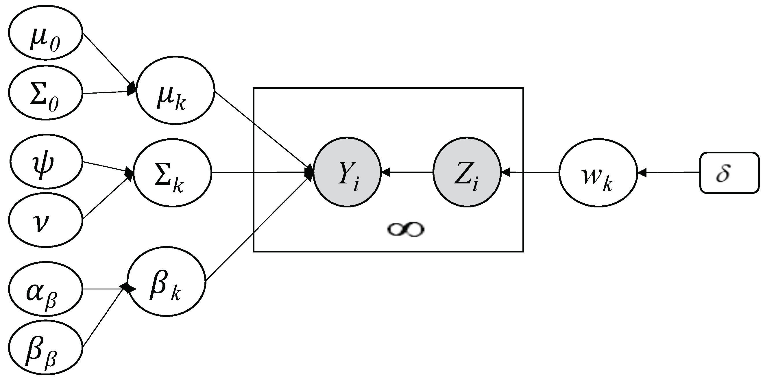
2.2. Model Specification

We start by recalling here the finite mixture of K multivariate generalized Normal distributions (MGND).

Definition 1

(Multivariate generalized Normal distribution). We say that $\overrightarrow{Y}$, D-dimensional vector, has a multivariate generalized Normal distribution with parameters $(\overrightarrow{\mu };\mathsf{\Sigma };\beta )$ and noted as $\overrightarrow{Y}\sim MG{N}^D(\overrightarrow{\mu };\mathsf{\Sigma };\beta )$, if its density function is defined as [10]:

$$p(\overrightarrow{Y}|\theta )=p(\overrightarrow{Y}|\overrightarrow{\mu };\mathsf{\Sigma };\beta )=\frac{\mathsf{\Gamma }\left(\frac{d}{2}\right)}{{\pi }^{\frac{d}{2}}\mathsf{\Gamma }\left(\frac{d}{2\beta }\right)2^{\frac{d}{2\beta }}}\frac{\beta }{{\left|\mathsf{\Sigma }\right|}^{\frac{1}{2}}}exp\left[-\frac{1}{2}{({(\overrightarrow{Y}-\overrightarrow{\mu })}^T{\mathsf{\Sigma }}^{-1}(\overrightarrow{Y}-\overrightarrow{\mu }))}^{\beta }\right].$$

(1)

For the case of finite mixtures, we suppose that we have K components following a multivariate generalized Normal distribution. Let $\mathcal{Y}$ set of vectors, such as $\mathcal{Y}=\{{\overrightarrow{Y}}_1,{\overrightarrow{Y}}_2,\dots ,{\overrightarrow{Y}}_N\}$, be a realization from K mixture components. Here the ${\overrightarrow{Y}}_n=(x_{n1},\dots ,x_{nD})$ is D-dimensional. Thus, the likelihood is defined as follows [4]:

$$p\left(\mathcal{Y}\right|\mathsf{\Theta })=\prod _{n=1}^N\sum _{k=1}^K{w}_{k}p({\overrightarrow{Y}}_n|{\theta }_k),$$

(2)

where $\mathsf{\Theta }=(\overrightarrow{w},\theta )$. $p({\overrightarrow{Y}}_n|{\theta }_k)$ is the $k^{th}$ component of the mixture defined by its parameters ${\theta }_k=({\overrightarrow{\mu }}_k,{\mathsf{\Sigma }}_k,{\beta }_k)$. Here, $\left\{w_k\right\}$ is a mixing weight parameter that satisfies $0\le w_k\le 1$ together with ${\sum }_{k=1}^K{w}_k=1$.

• ${\overrightarrow{\mu }}_k$ is the mean vector of the MGGD distribution.
• ${\beta }_k$ represents its shape parameter. It inspects the peakedness and the spread of the distribution.
• ${\mathsf{\Sigma }}_k$ is its covariance matrix, also called a scatter matrix.

It is noted that each ${\overrightarrow{Y}}_n$ is generated from one component.

2.3. The Infinite Mixture Model

In recent years, many nonparametric Bayesian methods have been developed in order to build more realistic and more flexible statistical mixture models. In this case, parameters are considered random and follow specific probability distributions (known as prior distributions), allowing us to describe our knowledge before seeing the data, and to update our prior beliefs, the likelihood is used. On the other hand, nonparametric Bayesian models have the advantage of allowing an infinite number of clusters, so there is no constraint on this number, and they are therefore considered more suitable for modeling, in particular with dynamic data. Thus, the number of parameters may increase or decrease as we have new data. With an infinite mixture, we can overcome the limits of the finite models, which are highly restrictive and then we effectively take into account the uncertainty of the model (the data come from an infinite number of clusters). In what follows, we will show how infinite mixture models have the ability to generate new clusters or delete some of existing ones when new data arrive. The model learning is based on building estimates of the posterior distribution for our infinite multivariate generalized Normal mixture model using the Monte Carlo Markov Chain (MCMC) technique [15,29]. Given that the calculation of posterior distributions is intractable for the case of mixture models, it is therefore recommended to implement effective approximation tools to generate samples from these posterior distributions. In this work, we are motivated to apply the well known Gibbs sampler [11,30] to generate posterior samples. In what follows, we focus on developing the priors and conditional posteriors needed to run Gibbs sampling.

2.3.1. Priors and Conditional Posterior Distributions

In contrast to deterministic approximation, which is generally based on the EM algorithm—where the missing data noted by $\mathcal{Z}=({\overrightarrow{Z}}_1,\dots ,{\overrightarrow{Z}}_N)$ where ${\overrightarrow{Z}}_i=(Z_{i1},\dots ,Z_{iK})$ for i = 1, …—the N. Bayesian approach to mixture learning is more efficient. Indeed, it is able to overcome the drawbacks related to the deterministic methods (maximum likelihood-based technique) such as its convergence to local maxima and their tendency to overfit noisy and sparse data. In the following, we develop our fully nonparametric Bayesian approach for learning the infinite multivariate generalized Normal mixture model (inMGNMM). Thus, the likelihood of complete data (both observed and missing) is expressed as:

$$p(\mathcal{Y},\mathcal{Z}|\mathsf{\Theta })=\prod _{n=1}^N\prod _{k=1}^K{(w_{k}p({\overrightarrow{Y}}_n|{\theta }_k))}^{Z_{nk}}.$$

(3)

The role of the likelihood is to update the prior knowledge as regards the parameters of the model ($p\left(\mathsf{\Theta }\right)$). Then, the priors on the model parameters will be updated and expressed in terms of posterior knowledge $p\left(\mathsf{\Theta }\right|\mathcal{Y},\mathcal{Z})$. By exploiting the Bayes’ rule, we have the following relationship between priors, likelihood and posteriors [4]:

$$p\left(\mathsf{\Theta }\right|\mathcal{Z},\mathcal{Y})=\frac{p(\mathcal{Z},\mathcal{Y}|\mathsf{\Theta }\left)p\right(\mathsf{\Theta })}{\int p(\mathcal{Z},\mathcal{Y}|\mathsf{\Theta }\left)p\right(\mathsf{\Theta })}\propto p(\mathcal{Z},\mathcal{Y}|\mathsf{\Theta })p\left(\mathsf{\Theta }\right),$$

(4)

where $(\mathcal{Z},\mathcal{Y}),p\left(\mathsf{\Theta }\right)$ and $p\left(\mathsf{\Theta }\right|\mathcal{Z},\mathcal{Y})$ are the complete data, the prior information about the model’s parameters and the posterior, respectively. It is important to note that the choice of the priors is one of the crucial aspects of Bayesian modeling and directly influences the final results [31]. The provided observed data will certainly improve these priors. In what follows, selecting and specifying the best choice for priors is covered as well as the finding of the underlying equations for the posteriors. After that, we will simulate a value very close to the truth for $\mathsf{\Theta }\sim p\left(\mathsf{\Theta }\right|\mathcal{Z},\mathcal{Y})$ by applying the efficient Gibbs sampler algorithm. In the current work, we choose priors for the parameters of the proposed model as follows:

• We start by specifying a common prior for ${\overrightarrow{\mu }}_j$ as a Normal distribution, thus we have ${\overrightarrow{\mu }}_j\sim \mathcal{N}({\overrightarrow{\mu }}_0,{\mathsf{\Sigma }}_0)$.
• For the shape parameter $,{\beta }_j$, an appropriate prior is the Gamma distribution (${\beta }_j\sim \mathcal{G}({\alpha }_{\beta },{\beta }_{\beta })$).
• For the covariance matrix ${\mathsf{\Sigma }}_j$, a natural prior choice is the Inverted Wishart (${\mathsf{\Sigma }}_j\sim IW(\psi ,\nu )$).

Having all these prior distributions, we move now to calculate all conditional posterior distributions based on the Bayes’ theorem.

-

The conditional posterior distribution for the mean parameter is determined as:

$$\begin{array}{cc}\hfill & p\left({\overrightarrow{\mu }}_j\right|\mathcal{Z},\mathcal{Y})\propto p\left({\overrightarrow{\mu }}_j\right)\prod _{Z_{ij}=1}p\left({\overrightarrow{Y}}_i\right|{\overrightarrow{\mu }}_j,{\beta }_j,{\mathsf{\Sigma }}_j)\hfill \\ \hfill & \propto \mathcal{N}({\overrightarrow{\mu }}_0,{\mathsf{\Sigma }}_0)\prod _{Z_{ij}=1}p\left({\overrightarrow{Y}}_i\right|{\overrightarrow{\mu }}_j,{\beta }_j,{\mathsf{\Sigma }}_j)\hfill \\ \hfill & \propto exp(-\frac{1}{2}{({\overrightarrow{\mu }}_j-{\overrightarrow{\mu }}_0)}^T{\mathsf{\Sigma }}_0^{-1}({\overrightarrow{\mu }}_j-{\overrightarrow{\mu }}_0))\times \hfill \\ \hfill & exp\left(\sum _{Z_{ij}=1}(\frac{-1}{2m^{{\beta }_j}}{({({\overrightarrow{Y}}_i-{\overrightarrow{\mu }}_j)}^T{\mathsf{\Sigma }}_j^{-1}({\overrightarrow{Y}}_i-{\overrightarrow{\mu }}_j))}^{{\beta }_j})\right).\hfill \end{array}$$

(5)

-

The conditional posterior distribution for the shape parameter is determined as:

$$\begin{array}{cc}\hfill & p\left({\beta }_j\right|\mathcal{Z},\mathcal{Y})\propto p\left({\beta }_j\right)\prod _{Z_{ij}=1}p\left({\overrightarrow{Y}}_i\right|{\overrightarrow{\mu }}_j,{\beta }_j,{\mathsf{\Sigma }}_j)\hfill \\ \hfill & \propto \mathcal{G}({\alpha }_{\beta },{\beta }_{\beta })\prod _{Z_{ij}=1}p\left({\overrightarrow{Y}}_i\right|{\overrightarrow{\mu }}_j,{\beta }_j,{\mathsf{\Sigma }}_j)\hfill \\ \hfill & \propto {\beta }_j^{{\alpha }_{\beta }-1}{e}^{-{\beta }_{\beta }{\beta }_j}{\left(\frac{{\beta }_j}{\mathsf{\Gamma }(d/2{\beta }_j)2^{d/2{\beta }_j}}\right)}^{n_j}\times \hfill \\ \hfill & exp\left(\sum _{Z_{ij}=1}(\frac{-1}{2m^{{\beta }_j}}{({({\overrightarrow{Y}}_i-{\overrightarrow{\mu }}_j)}^T{\mathsf{\Sigma }}_j^{-1}({\overrightarrow{Y}}_i-{\overrightarrow{\mu }}_j))}^{{\beta }_j})\right).\hfill \end{array}$$

(6)

-

The conditional posterior distribution of covariance matrix is calculated as:

$$\begin{array}{cc}\hfill & p\left({\mathsf{\Sigma }}_j\right|\mathcal{Z},\mathcal{Y})\propto p\left({\mathsf{\Sigma }}_j\right)\prod _{Z_{ij}=1}p\left({\overrightarrow{Y}}_i\right|{\overrightarrow{\mu }}_j,{\beta }_j,{\mathsf{\Sigma }}_j)\hfill \\ \hfill & \propto IW(\psi ,\nu )\prod _{Z_{ij}=1}p\left({\overrightarrow{Y}}_i\right|{\overrightarrow{\mu }}_j,{\beta }_j,{\mathsf{\Sigma }}_j)\hfill \\ \hfill & \propto |{\mathsf{\Sigma }}_j{|}^{-(\nu +d+1)/2}{e}^{-1/2tr\left(\psi {\mathsf{\Sigma }}_j^{-1}\right)}\times \hfill \\ \hfill & exp\left(\sum _{Z_{ij}=1}(\frac{-1}{2m^{{\beta }_j}}{({({\overrightarrow{Y}}_i-{\overrightarrow{\mu }}_j)}^T{\mathsf{\Sigma }}_j^{-1}({\overrightarrow{Y}}_i-{\overrightarrow{\mu }}_j))}^{{\beta }_j})\right).\hfill \end{array}$$

(7)

As for the conditional posterior distribution of the mixing weight $\overrightarrow{w}$, we know that $\overrightarrow{w}$ is determined on the simplex $\{(w_1,\dots ,w_K):{\sum }_{j=1}^{K-1}{w}_k<1\}$, then, in order to account for the infinite mixture principle, a natural prior that we have to state is the Dirichlet distribution with parameters $\frac{\delta }{M}$ [20].

$$p\left(\overrightarrow{w}\right|\delta )=\frac{\mathsf{\Gamma }\left(\delta \right)}{{\prod }_{k=1}^K\mathsf{\Gamma }\left(\frac{\delta }{K}\right)}\prod _{k=1}^K{w}_k^{\frac{\delta }{K}-1}.$$

(8)

The inference of $\overrightarrow{w}$ is performed via the inference of the membership vectors ${\overrightarrow{Z}}_n$. Thus, we can deduce $p(\mathcal{Z}|\overrightarrow{w})$ as follows:

$$\begin{array}{cc}\hfill p\left(\mathcal{Z}\right|\overrightarrow{w})& =\prod _{n=1}^{N}p\left({\overrightarrow{Z}}_n\right|\overrightarrow{w})=\prod _{n=1}^N{w}_1^{Z_{i1}}\dots w_M^{Z_{nM}}\hfill \\ \hfill & =\prod _{n=1}^N\prod _{k=1}^K{w}_k^{Z_{nk}}=\prod _{k=1}^K{w}_k^{a_k},\hfill \end{array}$$

(9)

where $a_k$ represents the total elements in cluster k. When considering the Dirichlet integral, we will obtain $p\left(\mathcal{Z}\right|\eta )={\prod }_{n=1}^N\frac{\left({\sum }_{l<n}{\mathbb{I}}_{{\overrightarrow{Z}}_n={\overrightarrow{Z}}_l}\right)+\frac{\delta }{K}}{\left(\right(n-1)+\delta )}$. For ${\overrightarrow{Y}}_l$, $l=1,\dots ,n-1$, the conditional prior that $\overrightarrow{X_n}$ to be in component k is given as [32]:

$$p(Z_{nk}=1|\delta ;{\overrightarrow{Z}}_1,\dots ,{\overrightarrow{Z}}_{n-1})=\frac{{\sum }_{l<n}{\mathbb{I}}_{{\overrightarrow{Z}}_n={\overrightarrow{Z}}_l}+\frac{\delta }{K}}{n-1+\delta }.$$

(10)

In order to N vectors, Equation (10) is updated as follows [32]:

$$p(Z_{nk}=1|\delta ;{\mathcal{Z}}_{-n})=\frac{a_{-nk}+\frac{\delta }{K}}{N-1+\delta },$$

(11)

where ${\mathcal{Z}}_{-n}=\{{\overrightarrow{Z}}_1,\dots ,{\overrightarrow{Z}}_{n-1},{\overrightarrow{Z}}_{n+1},\dots ,{\overrightarrow{Z}}_N\}$, $a_{-nk}$ is the number of vectors, excluding ${\overrightarrow{Y}}_i$, in cluster j. It is then necessary to calculate the conditional posterior by multiplying the prior (Equation (11)) by the likelihood ${\overrightarrow{Y}}_i$.

Remember that, in order to deploy mixture models, we have to define the number of components (called the model’s complexity), which is always a difficult question. In our nonparametric case, we initially assume an infinite number of clusters by making $K\to \infty$ in Equation (11). So, the conditional prior becomes [20,32]:

$$p(Z_{nk}=1|\delta ;{\mathcal{Z}}_{-n})=\left\{\begin{array}{cc}\frac{a_{-nk}}{N-1+\delta }& \mathrm{if} a_{-nk}>0 \mathrm{if} k\in represented clusters(\mathcal{R})\\ \frac{\delta }{N-1+\delta }& \mathrm{if} a_{-nk}=0 \mathrm{if} k\in unrepresented clusters(\mathcal{U})\\ ,\end{array}\right.$$

(12)

where the represented clusters are denoted by $\mathcal{R}$ and the unrepresented clusters are denoted by $\mathcal{U}$. Once the conditional priors in Equation (12) are evaluated, we now calculate the posterior using the following resulting equation [32]:

$$\begin{array}{ccc}\hfill & & p(Z_{nk}=1|{\overrightarrow{\mu }}_k,{\beta }_k,{\mathsf{\Sigma }}_k,{\overrightarrow{w}}_k,\delta ;{\mathcal{Z}}_{-n})\hfill \\ \hfill & =& \left\{\begin{array}{cc}\frac{a_{-nk}}{N-1+\delta }p\left({\overrightarrow{Y}}_n\right|{\overrightarrow{\mu }}_k,{\beta }_k,{\mathsf{\Sigma }}_k,{\overrightarrow{w}}_k)& \mathrm{if} k\in \mathcal{R}\\ \int \frac{\delta p\left({\overrightarrow{Y}}_n\right|{\overrightarrow{\mu }}_k,{\beta }_k,{\mathsf{\Sigma }}_k,{\overrightarrow{w}}_k)p\left({\overrightarrow{\mu }}_k\right)p\left({\beta }_k\right)p\left({\mathsf{\Sigma }}_k\right)p\left({\overrightarrow{w}}_k\right)}{N-1+\delta }d{\overrightarrow{\mu }}_{k}d{\beta }_{k}d{\mathsf{\Sigma }}_{k}d{w}_k& \mathrm{if} k\in \mathcal{U}\\ .\end{array}\right.\hfill \end{array}$$

(13)

Depending on a given probability, the former equation can be explained clearly by the fact that each vector is assigned to a represented or unrepresented cluster. If a vector is set for an unrepresented component, then we will create a new represented component all the time we have at least an empty cluster). This scenario explains the principle behind the countably infinite mixture well [20]. Our implemented Bayesian infinite model is illustrated in Figure 2. This figure shows the underlying graphical model.

2.3.2. Pseudo-Algorithm

After obtaining all necessary conditional posterior distributions, we consider the MCMC to estimate the underlying values. Here, the iterative Gibbs algorithm is executed [21] in order to sample the next unknown amounts from the conditional distributions given the values obtained previously. Our implemented pseudo-algorithm is summarized as follows:

• Generate ${\overrightarrow{Z}}_i$ from Equation (13), $i=1,\dots ,N$.
• Update the represented clusters denoted by M.
• Update $w_j=\frac{n_j}{N+\delta }$ and $n_j$, $j=1,\dots ,M$.
• Update the mixing parameters $w_U=\frac{\delta }{\delta +N}$.
• Update ${\overrightarrow{\mu }}_k$, ${\beta }_k$ and ${\mathsf{\Sigma }}_k$ using the underlying posteriors, $k=1,\dots ,K$.

It is worth noting that, during the initialization step, the algorithm starts by supposing that all the vectors are in the same cluster. Moreover, the initial values for the model’s parameters are supposedly produced from their prior distribution. To sample the vectors $Z_i$, it is required to compute the integral in Equation (13); however, this quantity is not analytically tractable. To deal with this issue, we propose to apply an efficient algorithm named “Metropolis-Hastings algorithm (M-H)”. The latter has the advantage of making the right decision to accept or reject the new samples—at iteration (t)—using an acceptance rate defined as follows:

$$r=\frac{p\left({\tilde{\mathsf{\Theta }}}_j\right|\mathcal{Z},\mathcal{Y})q\left({\mathsf{\Theta }}_j^{(t-1)}\right|{\tilde{\mathsf{\Theta }}}_j)}{p\left({\mathsf{\Theta }}_j^{(t-1)}\right|\mathcal{Z},\mathcal{Y})q\left({\tilde{\mathsf{\Theta }}}_j\right|{\mathsf{\Theta }}_j^{(t-1)})},$$

(14)

where q is the target distribution. In order to deal with the convergence problem with MCMC inference (in other words, how much the MCMC has to be executed), this problem is addressed, as in [33], to stop sampling and by applying a successful algorithm named one long-run with diagnostics [34].

3. Experiments

The goal of the following experiments is to evaluate the proposed framework and to compare the performance of the infinite multivariate generalized Normal mixture to its counterpart finite model and also to other models. We are primarily concerned with two challenging applications, namely texture classification and human activity categorization. For each of these, we have run ten chains with varying initial parameter values and have considered 10,000 iterations for the Metropolis-within-Gibbs sampler. Convergence was assessed using the diagnostic procedures, as in [35]. For all models tested, we discarded the first 1000 iterations as “burn-in” and kept the remaining 9000 iterations, from which we calculated the posteriors.

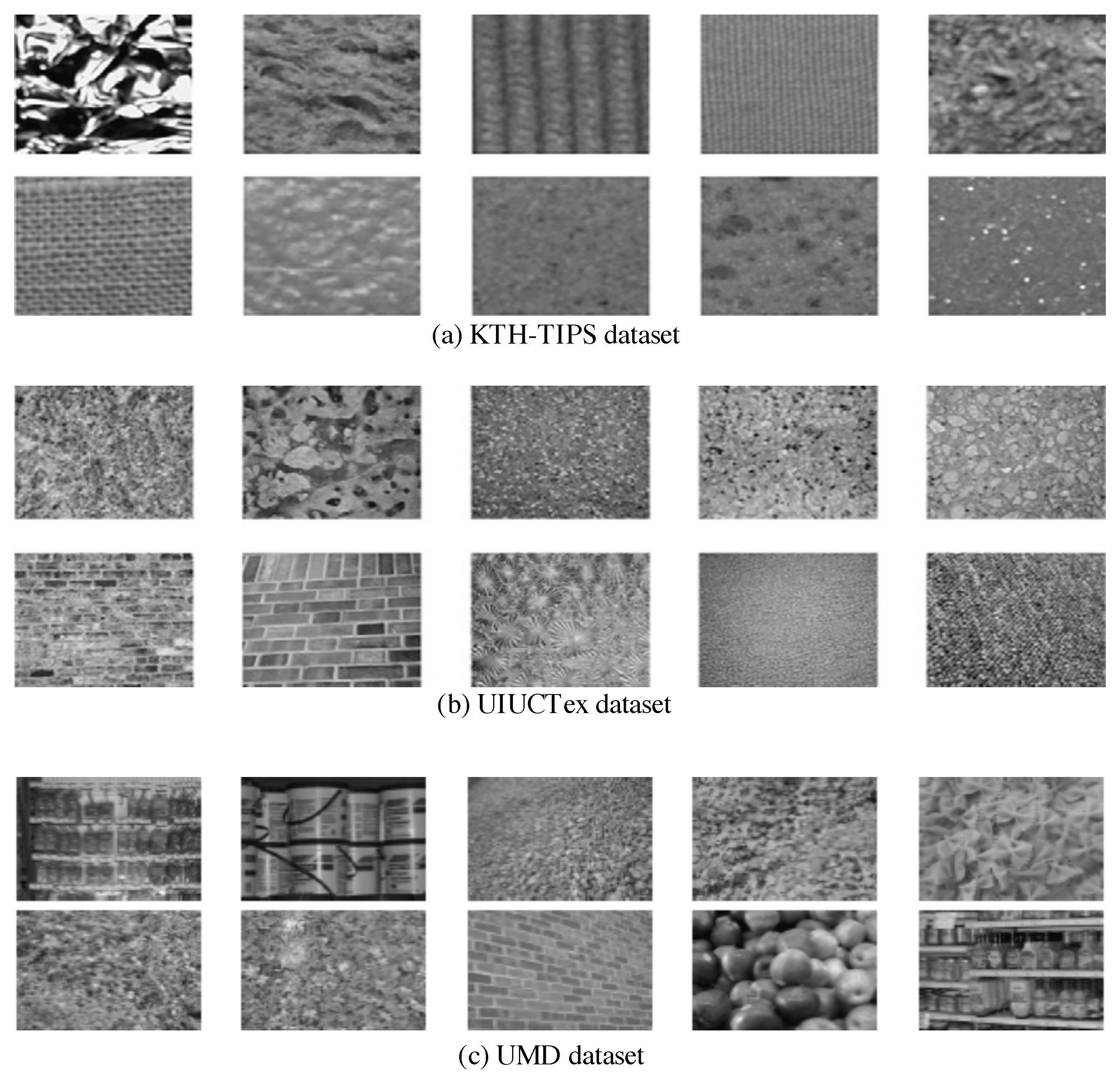
3.1. Texture Classification

First of all, we are motivated by the problem of texture images’ modeling and categorization. Unlike natural images, which include certain objects and structures, texture images are a special category of images and do not have a well defined shape. Texture characteristics play an important role in visual content analysis and are a well-studied property of images. It has been widely exploited before as an important indicator for the categorization and classification of images [36,37,38,39]. A number of computer vision applications use the texture information such as information retrieval, material classification [40], object detection [37,41], image segmentation [36,42,43] and facial expression recognition [38]. Previous texture extraction techniques have been mainly based on Gray Level Co-occurring Histograms [44], Local Binary Pattern (LBP) [45] and different filter banks [46]. An in-depth examination of these approaches is beyond the scope of our study. Instead, we are focusing on an efficient technique to extract relevant texture features and this technique has produced interesting results (DMD) [25]. It is based on the representation of texture using a set of local features called dense micro-block difference (DMD). The obtained features do not involve any quantization, thus retaining the complete information. In addition, these features do not involve any thresholding step and have the advantage of being quick and simple, like binary features. They are capable of achieving high discrimination and are considered invariant with respect to orientation, scale and resolution. After extracting these features, we encode them using a Fisher vector method [25] to obtain a set of descriptors of the underlying image. Thus, each image is represented by a robust multidimensional vector of descriptors that involve high-order statistics (the Matlab code for the features is available at http://www.cs.tut.fi/~mehta/texturedmd (accessed on 1 February 2021)). The last step is to classify the resulting descriptors using a linear support vector machine classifier, which results in the categorization of texture images into homogeneous categories. In all our experiments, we use a linear SVM classifier, which is able to directly operate on the vector of features and also requires less training time over other SVM kernels. The performance study is reported in terms of accuracy based on 10 fold cross validation.

Experimental evaluation involves the following texture databases. The first dataset, named UIUCTex [47], contains 25 texture classes and each one includes 40 images, thus, each has 40,640 × 480 pixel images. The textures of this dataset are taken under different scales and viewpoint changes, including non-rigid deformations. The second dataset, named KTH-TIPS [40], contains images of ten classes (materials) and each one includes 81 images (200 × 200 pixel ) per class. Images are captured with different combinations such as nine different scales, viewed under three different poses and illumination directions. The third dataset is the UMD dataset [48], which is composed of 25 textures classes including 40 samples (with resolution of 1280 × 900) per each texture-class (a total number of 25 × 40 = 1000 uncalibrated images). Images are captured under different significant distances and viewing directions, and the illuminations are uncontrolled.

Figure 3 shows random samples of textured images from different classes presenting in the three datasets. For all these databases, 50% of images are randomly chosen for training and 50% for testing. In order to quantify how well textures are classified, we evaluate the performance with an accuracy metric. To validate our approach (inMGNMM), we compared it with five other methods, namely finite Gaussian mixture (GMM), infinite Gaussian mixture (inGMM), finite generalized Gaussian mixture (GGMM), infinite generalized Gaussian mixture (inGGMM), and finite multivariate generalized Gaussian mixture (MGGMM) [10].

The evaluation results using three different datasets for six different methods are summarized in

Table 1. Overall classification accuracy rate (%) of different approaches for the three texture datasets using SIFT features.

Method	KTH-TIPS	UIUCTex	UMD
GMM	80.22	84.64	83.70
inGMM	80.94	85.33	84.14
GGMM	82.11	86.51	86.42
inGGMM	83,30	87.21	87.17
MGGMM [10]	84.10	88.09	88.15
inMGNMM (our method)	85.91	89.03	89.10

,

Table 2. Overall classification accuracy rate (%) of different approaches for the three texture datasets using LBP features.

Method	KTH-TIPS	UIUCTex	UMD
GMM	80.88	84.98	83.99
inGMM	81.24	86.03	84.84
GGMM	82.90	87.05	86.96
inGGMM	83.94	87.84	87.86
MGGMM [10]	84.81	88.78	88.87
inMGNMM (our method)	86.29	89.81	89.97

and

Table 3. Overall classification accuracy rate (%) of different approaches for the three texture datasets using DMD features.

Method	KTH-TIPS	UIUCTex	UMD
GMM	83.08	87.77	86.12
inGMM	84.13	89.77	87.12
GGMM	85.76	90.02	89.75
inGGMM	86.88	90.67	90.20
MGGMM [10]	87.67	91.07	91.23
inMGNMM (our method)	88.91	92.11	92.12

, respectively. Accordingly, it is clear that our method has the highest achieved accuracy for the three datasets. In particular, for the case of the UMD dataset, the accuracy of our infinite mixture with DMD features is 92.12% and, therefore, it outperforms the other methods—GMM, inGMM, GGMM and inGGMM by—6%, 5%, 2.37% and 1.92%, respectively. Likewise, we reached the same conclusion for other datasets, and our model provides very encouraging results using different features as compared to other models. By contrast, the worst performance is obtained with the Gaussian-based classification. We can also conclude that all obtained results using our proposed infinite mixture are increased by around 1% to 2% if comparing it to its finite mixture counterpart (MGGMM). This can be explained by the model’s capacity to combine prior knowledge during the learning process, its generalization capability, and its flexibility in terms of making less restrictive assumptions about the number of clusters than the finite model. On the other hand, a superior performance of the visual feature DMD over the SIFT and LBP for texture classification task can be observed in all these datasets. With DMD, the accuracy is improved over SIFT and LBP by around 3% and 2%, respectively. This result is probably achieved by the rich description of DMD obtained by considering all possible fine details at different resolutions and scales. Finally, we note that the performance of all methods for the KTH-TIPS dataset indicates that it is sometimes difficult to identify texture because of its various rotation and viewpoint changes.

3.2. Human Actions Categorization

Recently, multimedia categorization and recognition are becoming two challenging research problems that have attracted a lot of attention for several applications [49,50,51,52]. Object categorization refers to the task of labelling objects into one of the predefined and meaningful categories and this step is mainly based on extracting effective visual features. Image categorization plays an essential role in many applications such as automatic organization, activity recognition, object retrieval and tracking. In particular, recognizing human activities (HAR) is extremely recommended for security purposes (video surveillance), health care, robotics, and so forth. The objective is to identify the actions of one or more persons and then to analyze them [53]. It is worth noting that manually categorizing a big dataset is impractical and time consuming. Recently, various automatic and semi-automatic methods have been developed to address this problem [10,12,54,55,56]. For instance, a finite generalized Gaussian mixture model is investigated to deal with HAR through a complex real dataset [10,12,52]. In [57], the authors developed an algorithm to identify human gestures using features derived from key poses. A Hidden Markov Model is also presented for HAR in [58]. It is noted that, for a human, a simple glance is enough to classify or categorize any action. Nevertheless, exact and accurate categorization with a computer (or algorithm) is a very difficult task and it will be more complex in the presence of illumination, occlusions, lighting, noise, the and absence of a large amount of labelled data. Thus, increasing attention has been paid to unsupervised machine learning methods, which are able to learn objects from unlabelled data. Furthermore, implementing more advanced computational intelligence techniques is required to solve the above issues and to achieve higher recognition rates.

In this work, our contribution consists of exploiting our approach for human activity categorization and recognition. For this goal, the KTH human action dataset [59] was used to evaluate its performance. Some samples of representative actions with four scenarios are presented in Figure 4. These scenarios are outdoors (s1), outdoors with scale variation (s2), outdoors with different clothes (s3) and indoors (s4). The dataset basically contains 2391 sequences with different actions that are grouped into six categories—running, boxing, walking, jogging, hand waving and hand clapping.

Before we applied our model to categorize actions, we basically adopted a few useful preprocessing steps. Fist, a visual vocabulary was constructed by adopting the bag-of-words (BOW) model representation for the input training sequences. Indeed, each sequence would be defined by a set of local SIFT3D descriptors [60]. These features were then quantized as visual words via the K-means algorithm [61]. We then had a frequency histogram over the visual words. After that, we applied a probabilistic Latent Semantic Analysis (pLSA) [62] method on the obtained frequency histograms to generate a d-dimensional vector for each image. This final representation would then be used for unsupervised activity categorization.

In order to assess the performance of the proposed approach, we adopted the accuracy metric as a recognition rate for human action categorization. To test the efficiency of our method, we used a five-fold cross-validation setup. For evaluation purposes, we compared the proposed approach with several state-of-the-art methods as depicted in

Table 4. Comparative study for Human Activity Recognition between different approaches for the KTH database.

Method	Recognition Rate (%)
GMM-FS	72.51
GMM-KL	77.77
GGMM-FS	73.89
GGMM-KL	78.05
SVM-Linear	73.24
SVM-Polynomial	71.44
SVM-Radial basis	79.33
Niebles et al. [63]	83.33
Wong et al. [64]	73.24
Fan et al. [65]	79.33
Schuldt et al. [59]	71.71
Dolar et al. [66]	78.50
MGGMM-FS [10]	82.01
MGGMM-KL [10]	82.36
inMGNMM (our method)	84.68

. According to this comparative study, we can clearly see that our approach provides the best recognition rate (84.68%) compared to the other methods. This result is considered very encouraging given that we approached the recognition problem in an unsupervised manner. The superior performance of the proposed infinite model over its finite counterpart (82.01%) is also clear. This result proves that the infinite mixtures are more attractive and flexible enough to be applied to recognition problems. We report that the developed framework does not take into account any background tracking or subtraction and, for this reason, the accuracy is considered quite high. Note that sometimes we are not able to recognize very similar actions such as those involving hand motions. To improve these findings, it may be interesting to simultaneously incorporate a feature selection process into the developed statistical learning model.

4. Discussion

The experiments conducted show the superiority of our approach over other state-of-the-art statistical models and methods. Indeed, the obtained results show the benefits of our model and prove the flexibility of the implemented statistical framework. In particular, we obtain a better performance within the descriptor DMD (in terms of accuracy). However, it is important to note that some poor results are obtained (for all involved methods in this work) and this can probably be explained by the difficulty of identifying the exact texture class due to its different rotations and changes in viewpoints. One possible solution, which we are starting to work on, is to introduce a feature selection mechanism, as in [67,68], to improve the classification performance. Another challenge we face with our method is to fine-tune hyperparameters that may have an impact on classification and recognition accuracy. It is also important to note that the quality of images used for validation purposes may be affected by uncertainties and/or inaccuracies that would make the edges not perfectly distinguishable. In these cases, it would be necessary to use fuzzy preprocessing of the images, as done in [69,70]. On the other hand, Bayesian classification by infinite mixture models is also noted to be interesting due to its efficient MCMC sampling technique; however, it is problematic because of its high computational cost. In particular, we run the Gibbs algorithm several times to achieve a correct average accuracy. Therefore, one potential for future work might be to extend this work to use variable inference instead, in order to save time over MCMC methods. Finally, it may be important to apply the proposed work to more complicated and challenging machine vision datasets for further performance evaluation.

5. Conclusions

We have proposed in this paper an effective hierarchical nonparametric statistical Bayesian framework that tackles complex data modeling, categorization and classification. The proposed framework is based on a mixture of multivariate generalized Normal distributions (MGNMM). The main goal here is to extend the finite MGNMM to the infinite case (inMGNMM), in which the number of components is supposed to be infinite initially and will be inferred automatically during the learning and modeling of classes. The success of the nonparametric Bayesian learning approach is due to the appropriate choice of priors and the accurate posterior estimates via MCMC simulations. The proposed inMGNMM is learned through MCMC inference. This learning algorithm is guaranteed to converge and has the advantage of taking into account our prior knowledge, to formalize our uncertainty via flexible probability distributions, and to overcome the over-fitting issue. Our choice of the infinite assumption, instead of the finite, is motivated by the fact it is able to learn the number of components (i.e., model selection) and the parameters at the same time. The implemented framework allows for the logical treatment of determining the optimal number of components and the efficient estimation of the parameters’ values. The effectiveness of the developed approach is confirmed by testing it on two challenging computer vision applications, namely texture classification and human activities categorization. Extensive experiments were conducted and the results demonstrate that the proposed approach outperforms the state-of-the-art on a number of datasets. These results prove the coherence, effectiveness and flexibility of our approach. Future works could be devoted to extending the current Bayesian work by integrating a feature selection mechanism, which could further enhance the expected results. It is also our hope that many other real-world image/signal processing problems can be tackled within the proposed approach. Finally, we plan to extend the current work by implementing a variational inference model in order to overcome the computational complexity of the Bayesian approach.

References

1. Li, Y.; Wang, G.; Li, M.; Li, J.; Shi, L.; Li, J. Application of CT images in the diagnosis of lung cancer based on finite mixed model. Saudi J. Biol. Sci. 2020, 27, 1073–1079. [Google Scholar] [CrossRef]
2. Lai, Y.; Ping, Y.; He, W.; Wang, B.; Wang, J.; Zhang, X. Variational Bayesian inference for finite inverted Dirichlet mixture model and its application to object detection. Chin. J. Electron. 2018, 27, 603–610. [Google Scholar] [CrossRef]
3. Bourouis, S.; Sallay, H.; Bouguila, N. A Competitive Generalized Gamma Mixture Model for Medical Image Diagnosis. IEEE Access 2021, 9, 13727–13736. [Google Scholar] [CrossRef]
4. McLachlan, G.J.; Peel, D. Finite Mixture Models; John Wiley & Sons: Hoboken, NJ, USA, 2004. [Google Scholar]
5. Bouguila, N.; Ziou, D. MML-Based Approach for Finite Dirichlet Mixture Estimation and Selection. In Machine Learning and Data Mining in Pattern Recognition, Proceedings of the 4th International Conference, MLDM 2005, Leipzig, Germany, 9–11 July 2005; Lecture Notes in Computer Science; Proceedings; Perner, P., Imiya, A., Eds.; Springer: Berlin/Heidelberg, Germany, 2005; Volume 3587, pp. 42–51. [Google Scholar] [CrossRef]
6. Khan, A.M.; El-Daly, H.; Rajpoot, N.M. A Gamma-Gaussian mixture model for detection of mitotic cells in breast cancer histopathology images. In Proceedings of the 21st International Conference on Pattern Recognition, ICPR 2012, Tsukuba, Japan, 11–15 November 2012; pp. 149–152. [Google Scholar]
7. Alroobaea, R.; Rubaiee, S.; Bourouis, S.; Bouguila, N.; Alsufyani, A. Bayesian inference framework for bounded generalized Gaussian-based mixture model and its application to biomedical images classification. Int. J. Imaging Syst. Technol. 2020, 30, 18–30. [Google Scholar] [CrossRef]
8. Bourouis, S.; Channoufi, I.; Alroobaea, R.; Rubaiee, S.; Andejany, M.; Bouguila, N. Color object segmentation and tracking using flexible statistical model and level-set. Multimed. Tools Appl. 2021, 80, 5809–5831. [Google Scholar] [CrossRef]
9. Bouchard, G.; Celeux, G. Selection of Generative Models in Classification. IEEE Trans. Pattern Anal. Mach. Intell. 2006, 28, 544–554. [Google Scholar] [CrossRef]
10. Najar, F.; Bourouis, S.; Bouguila, N.; Belghith, S. A new hybrid discriminative/generative model using the full-covariance multivariate generalized Gaussian mixture models. Soft Comput. 2020, 24, 10611–10628. [Google Scholar] [CrossRef]
11. Elguebaly, T.; Bouguila, N. A hierarchical nonparametric Bayesian approach for medical images and gene expressions classification. Soft Comput. 2015, 19, 189–204. [Google Scholar] [CrossRef]
12. Najar, F.; Bourouis, S.; Bouguila, N.; Belghith, S. Unsupervised learning of finite full covariance multivariate generalized Gaussian mixture models for human activity recognition. Multim. Tools Appl. 2019, 78, 18669–18691. [Google Scholar] [CrossRef]
13. Alharithi, F.S.; Almulihi, A.H.; Bourouis, S.; Alroobaea, R.; Bouguila, N. Discriminative Learning Approach Based on Flexible Mixture Model for Medical Data Categorization and Recognition. Sensors 2021, 21, 2450. [Google Scholar] [CrossRef] [PubMed]
14. Bouguila, N.; Almakadmeh, K.; Boutemedjet, S. A finite mixture model for simultaneous high-dimensional clustering, localized feature selection and outlier rejection. Expert Syst. Appl. 2012, 39, 6641–6656. [Google Scholar] [CrossRef]
15. Robert, C.; Casella, G. Monte Carlo Statistical Methods; Springer: New York, NY, USA, 2004. [Google Scholar]
16. Bourouis, S.; Laalaoui, Y.; Bouguila, N. Bayesian frameworks for traffic scenes monitoring via view-based 3D cars models recognition. Multim. Tools Appl. 2019, 78, 18813–18833. [Google Scholar] [CrossRef]
17. Chen, J.; Tan, X. Inference for multivariate normal mixtures. J. Multivar. Anal. 2009, 100, 1367–1383. [Google Scholar] [CrossRef] [Green Version]
18. Bourouis, S.; Bouguila, N. Nonparametric learning approach based on infinite flexible mixture model and its application to medical data analysis. Int. J. Imaging Syst. Technol. 2021. [Google Scholar] [CrossRef]
19. Fan, W.; Sallay, H.; Bouguila, N.; Bourouis, S. Variational learning of hierarchical infinite generalized Dirichlet mixture models and applications. Soft Comput. 2016, 20, 979–990. [Google Scholar] [CrossRef]
20. Rasmussen, C.E. The Infinite Gaussian Mixture Model. In Proceedings of the Advances in Neural Information Processing Systems (NIPS); MIT: Cambridge, MA, USA, November 2000; pp. 554–560. [Google Scholar]
21. Bouguila, N.; Ziou, D. A Dirichlet process mixture of generalized Dirichlet distributions for proportional data modeling. IEEE Trans. Neural Netw. 2010, 21, 107–122. [Google Scholar] [CrossRef]
22. Gelman, A.; Stern, H.S.; Carlin, J.B.; Dunson, D.B.; Vehtari, A.; Rubin, D.B. Bayesian Data Analysis; Texts in Statistical Science; Chapman and Hall/CRC: Boca Raton, FL, USA, 2013. [Google Scholar]
23. Bourouis, S.; Al-Osaimi, F.R.; Bouguila, N.; Sallay, H.; Aldosari, F.M.; Mashrgy, M.A. Bayesian inference by reversible jump MCMC for clustering based on finite generalized inverted Dirichlet mixtures. Soft Comput. 2019, 23, 5799–5813. [Google Scholar] [CrossRef]
24. Bourouis, S.; Alroobaea, R.; Rubaiee, S.; Andejany, M.; Almansour, F.M.; Bouguila, N. Markov Chain Monte Carlo-Based Bayesian Inference for Learning Finite and Infinite Inverted Beta-Liouville Mixture Models. IEEE Access 2021, 9, 71170–71183. [Google Scholar] [CrossRef]
25. Mehta, R.; Egiazarian, K.O. Texture Classification Using Dense Micro-Block Difference. IEEE Trans. Image Process. 2016, 25, 1604–1616. [Google Scholar] [CrossRef]
26. Boiman, O.; Shechtman, E.; Irani, M. In defense of Nearest-Neighbor based image classification. In Proceedings of the 2008 IEEE Computer Society Conference on Computer Vision and Pattern Recognition (CVPR 2008), Anchorage, AK, USA, 24–26 June 2008. [Google Scholar]
27. Jaakkola, T.S.; Haussler, D. Exploiting Generative Models in Discriminative Classifiers. In Advances in Neural Information Processing Systems 11, Proceedings of the NIPS Conference, Denver, CO, USA, 30 November–5 December 1998; Kearns, M.J., Solla, S.A., Cohn, D.A., Eds.; The MIT Press: Cambridge, MA, USA, 1998; pp. 487–493. [Google Scholar]
28. Sánchez, J.; Perronnin, F.; Mensink, T.; Verbeek, J.J. Image Classification with the Fisher Vector: Theory and Practice. Int. J. Comput. Vis. 2013, 105, 222–245. [Google Scholar] [CrossRef]
29. Marin, J.; Mengersen, K.; Robert, C. Bayesian modeling and inference on mixtures of distributions. In Handbook of Statistics 25; Dey, D., Rao, C., Eds.; Elsevier-Sciences: Amsterdam, The Netherlands, 2004. [Google Scholar]
30. Husmeier, D.; Penny, W.D.; Roberts, S.J. An empirical evaluation of Bayesian sampling with hybrid Monte Carlo for training neural network classifiers. Neural Netw. 1999, 12, 677–705. [Google Scholar] [CrossRef]
31. Geiger, D.; Heckerman, D. Parameter priors for directed acyclic graphical models and the characterization of several probability distributions. In Proceedings of the Fifteenth Conference on Uncertainty in Artificial Intelligence, Stockholm, Sweden, 30 July–1 August 1999; Morgan Kaufmann Publishers Inc.: San Francisco, CA, USA, 1999; pp. 216–225. [Google Scholar]
32. Neal, R.M. Markov chain sampling methods for Dirichlet process mixture models. J. Comput. Graph. Stat. 2000, 9, 249–265. [Google Scholar]
33. Roberts, G.O.; Tweedie, R.L. Bounds on regeneration times and convergence rates for Markov chainsfn1. Stoch. Process. Their Appl. 1999, 80, 211–229. [Google Scholar] [CrossRef]
34. Carlo, M. Comment: One Long Run with Diagnostics: Implementation Strategies for Markov Chain. Stat. Sci. 1992, 7, 493–497. [Google Scholar]
35. Cowles, M.K.; Carlin, B.P. Markov Chain Monte Carlo Convergence Diagnostics: A Comparative Review. J. Am. Stat. Assoc. 1996, 91, 883–904. [Google Scholar] [CrossRef]
36. Huang, Y.; Zhou, F.; Gilles, J. Empirical curvelet based fully convolutional network for supervised texture image segmentation. Neurocomputing 2019, 349, 31–43. [Google Scholar] [CrossRef]
37. Zhang, Q.; Lin, J.; Tao, Y.; Li, W.; Shi, Y. Salient object detection via color and texture cues. Neurocomputing 2017, 243, 35–48. [Google Scholar] [CrossRef]
38. Fan, W.; Bouguila, N. Online facial expression recognition based on finite Beta-Liouville mixture models. In Proceedings of the 2013 International Conference on Computer and Robot Vision, Regina, SK, Canada, 28–31 May 2013; pp. 37–44. [Google Scholar]
39. Zhao, G.; Pietikainen, M. Dynamic texture recognition using local binary patterns with an application to facial expressions. IEEE Trans. Pattern Anal. Mach. Intell. 2007, 29, 915–928. [Google Scholar] [CrossRef] [Green Version]
40. Hayman, E.; Caputo, B.; Fritz, M.; Eklundh, J. On the Significance of Real-World Conditions for Material Classification. In Computer Vision—ECCV 2004, Proceedings of the 8th European Conference on Computer Vision, Prague, Czech Republic, 11–14 May 2004; Pajdla, T., Matas, J., Eds.; Springer: Berlin/Heidelberg, Germany, 2004; Volume 3024, Part IV; pp. 253–266. [Google Scholar]
41. Zhang, J.; Marszalek, M.; Lazebnik, S.; Schmid, C. Local Features and Kernels for Classification of Texture and Object Categories: A Comprehensive Study. Int. J. Comput. Vis. 2007, 73, 213–238. [Google Scholar] [CrossRef] [Green Version]
42. Badoual, A.; Unser, M.; Depeursinge, A. Texture-driven parametric snakes for semi-automatic image segmentation. Comput. Vis. Image Underst. 2019, 188, 102793. [Google Scholar] [CrossRef]
43. Zheng, Y.; Chen, K. A general model for multiphase texture segmentation and its applications to retinal image analysis. Biomed. Signal Process. Control 2013, 8, 374–381. [Google Scholar] [CrossRef]
44. Haralick, R.M.; Shanmugam, K.S.; Dinstein, I. Textural Features for Image Classification. IEEE Trans. Syst. Man Cybern. 1973, 3, 610–621. [Google Scholar] [CrossRef] [Green Version]
45. Guo, Z.; Zhang, L.; Zhang, D. A Completed Modeling of Local Binary Pattern Operator for Texture Classification. IEEE Trans. Image Process. 2010, 19, 1657–1663. [Google Scholar] [PubMed] [Green Version]
46. Manjunath, B.S.; Ma, W. Texture Features for Browsing and Retrieval of Image Data. IEEE Trans. Pattern Anal. Mach. Intell. 1996, 18, 837–842. [Google Scholar] [CrossRef] [Green Version]
47. Lazebnik, S.; Schmid, C.; Ponce, J. A Sparse Texture Representation Using Local Affine Regions. IEEE Trans. Pattern Anal. Mach. Intell. 2005, 27, 1265–1278. [Google Scholar] [CrossRef] [Green Version]
48. Xu, Y.; Ji, H.; Fermüller, C. Viewpoint Invariant Texture Description Using Fractal Analysis. Int. J. Comput. Vis. 2009, 83, 85–100. [Google Scholar] [CrossRef]
49. Yao, Y.; Yang, W.; Huang, P.; Wang, Q.; Cai, Y.; Tang, Z. Exploiting textual and visual features for image categorization. Pattern Recognit. Lett. 2019, 117, 140–145. [Google Scholar] [CrossRef]
50. Traboulsi, Y.E.; Dornaika, F. Flexible semi-supervised embedding based on adaptive loss regression: Application to image categorization. Inf. Sci. 2018, 444, 1–19. [Google Scholar] [CrossRef]
51. Roy, S.; Shivakumara, P.; Jain, N.; Khare, V.; Dutta, A.; Pal, U.; Lu, T. Rough-fuzzy based scene categorization for text detection and recognition in video. Pattern Recognit. 2018, 80, 64–82. [Google Scholar] [CrossRef] [Green Version]
52. Najar, F.; Bourouis, S.; Zaguia, A.; Bouguila, N.; Belghith, S. Unsupervised Human Action Categorization Using a Riemannian Averaged Fixed-Point Learning of Multivariate GGMM. In Proceedings of the Image Analysis and Recognition—15th International Conference, ICIAR 2018, Póvoa de Varzim, Portugal, 27–29 June 2018; pp. 408–415. [Google Scholar]
53. Vrigkas, M.; Nikou, C.; Kakadiaris, I.A. A review of human activity recognition methods. Front. Robot. AI 2015, 2, 28. [Google Scholar] [CrossRef] [Green Version]
54. Zhu, R.; Dornaika, F.; Ruichek, Y. Learning a discriminant graph-based embedding with feature selection for image categorization. Neural Netw. 2019, 111, 35–46. [Google Scholar] [CrossRef]
55. Zhou, H.; Zhou, S. Scene categorization towards urban tunnel traffic by image quality assessment. J. Vis. Commun. Image Represent. 2019, 65, 102655. [Google Scholar] [CrossRef]
56. Sánchez, D.L.; Arrieta, A.G.; Corchado, J.M. Visual content-based web page categorization with deep transfer learning and metric learning. Neurocomputing 2019, 338, 418–431. [Google Scholar] [CrossRef]
57. Vieira, T.; Faugeroux, R.; Martínez, D.; Lewiner, T. Online human moves recognition through discriminative key poses and speed-aware action graphs. Mach. Vis. Appl. 2017, 28, 185–200. [Google Scholar] [CrossRef]
58. Zhu, C.; Sheng, W. Motion-and location-based online human daily activity recognition. Pervasive Mob. Comput. 2011, 7, 256–269. [Google Scholar] [CrossRef]
59. Schuldt, C.; Laptev, I.; Caputo, B. Recognizing human actions: A local SVM approach. In Proceedings of the 17th International Conference on Pattern Recognition, Cambridge, UK, 26 August 2004; Volume 3, pp. 32–36. [Google Scholar]
60. Scovanner, P.; Ali, S.; Shah, M. A 3-dimensional sift descriptor and its application to action recognition. In Proceedings of the 15th ACM international conference on Multimedia, Augsburg, Germany, 25 September 2007; pp. 357–360. [Google Scholar]
61. Csurka, G.; Dance, C.; Fan, L.; Willamowski, J.; Bray, C. Visual categorization with bags of keypoints. In Proceedings of the Workshop on Statistical Learning in Computer Vision, Prague, Czech Republic, 11–14 May 2004; Volume 1, pp. 1–2. [Google Scholar]
62. Bosch, A.; Zisserman, A.; Muñoz, X. Scene classification via pLSA. In Proceedings of the Computer Vision–ECCV, Graz, Austria, 7–13 May 2006; pp. 517–530. [Google Scholar]
63. Niebles, J.C.; Wang, H.; Fei-Fei, L. Unsupervised learning of human action categories using spatial-temporal words. Int. J. Comput. Vis. 2008, 79, 299–318. [Google Scholar] [CrossRef] [Green Version]
64. Wong, S.F.; Cipolla, R. Extracting spatiotemporal interest points using global information. In Proceedings of the 2007 IEEE 11th International Conference on Computer Vision. Citeseer, Rio de Janeiro, Brazil, 14–21 October 2007; pp. 1–8. [Google Scholar]
65. Fan, W.; Bouguila, N. Variational learning for Dirichlet process mixtures of Dirichlet distributions and applications. Multimed. Tools Appl. 2014, 70, 1685–1702. [Google Scholar] [CrossRef]
66. Dollár, P.; Rabaud, V.; Cottrell, G.; Belongie, S. Behavior Recognition via Sparse Spatio-Temporal Features; VS-PETS: Beijing, China, 2005. [Google Scholar]
67. Channoufi, I.; Bourouis, S.; Bouguila, N.; Hamrouni, K. Spatially Constrained Mixture Model with Feature Selection for Image and Video Segmentation. In Image and Signal Processing, Proceedings of the 8th International Conference, ICISP 2018, Cherbourg, France, 2–4 July 2018; Mansouri, A., Elmoataz, A., Nouboud, F., Mammass, D., Eds.; Springer: Berlin/Heidelberg, Germany, 2018; Volume 10884, pp. 36–44. [Google Scholar]
68. Fan, W.; Sallay, H.; Bouguila, N.; Bourouis, S. A hierarchical Dirichlet process mixture of generalized Dirichlet distributions for feature selection. Comput. Electr. Eng. 2015, 43, 48–65. [Google Scholar] [CrossRef]
69. Versaci, M.; Morabito, F.C. Image edge detection: A new approach based on fuzzy entropy and fuzzy divergence. Int. J. Fuzzy Syst. 2021, 23, 918–936. [Google Scholar] [CrossRef]
70. Orujov, F.; Maskeliunas, R.; Damasevicius, R.; Wei, W. Fuzzy based image edge detection algorithm for blood vessel detection in retinal images. Appl. Soft Comput. 2020, 94, 106452. [Google Scholar] [CrossRef]
Figure 1. The pipeline of the proposed method. First, robust invariant visual features are extracted from each image. Then, these features are modelled using an infinite multivariate generalized Normal mixture model. The next step consists of encoding them using Fisher vectors to obtain effective descriptors. Finally, an SVM classifier is applied for categorization and classification applications.
Applsci 11 05798 g001
Figure 2. Graphical representation of our developed Bayesian infinite multivariate generalized Normal mixture model. Fixed hyperparameters are indicated by rounded boxes and random variables by circles. Y is the observed variable, Z is the latent variable, large boxes indicate repeated process, and the arcs show the dependencies between variables.
Applsci 11 05798 g002
Figure 3. Samples of textures from different datasets (a) KTH-TIPS, (b) UIUCTex, and (c) UMD dataset.
Applsci 11 05798 g003
Figure 4. Sample frames of the KTH dataset actions with different scenarios.
Applsci 11 05798 g004