Comparative Analysis of Clustering Algorithms and Moodle Plugin for Creation of Student Heterogeneous Groups in Online University Courses

Abstract

Online learning environments such as e-learning platforms are often used to encourage collaborative activities amongst students. In this context, group work is often used to improve the learning outcomes. Group formation is often performed randomly since university courses can be composed of a large number of students. While random formation saves time and resources, the student heterogeneity in terms of learning capabilities is not guaranteed. Although advanced e-learning platforms such as Moodle are widely used, they lack plugins that allow the automatic formation of heterogeneous groups of students. This work proposes a novel intelligent plugin for Moodle that allows the creation of heterogeneous groups by using Machine Learning. This intelligent application can be used in order to improve the students’ performance in collaborative activities. Our machine learning approach first uses clustering algorithms on Moodle data to identify homogeneous groups that are composed of students having similar behavior. Heterogeneous groups are then created by combining students selected from different homogeneous groups. To this end, a novel algorithm and the corresponding software, which allow the creation of heterogeneous groups, have been developed. We have implemented our approach by realizing a Moodle plugin where teachers can create heterogeneous groups.

1. Introduction

Collaborative activities are a significant teaching methodology for students, as they improve learning outcomes by promoting active learning [1]. Collaboration also allows students to develop their social skills, such as decision making, communication, collaborative skills, and critical thinking [2,3,4]. Due to the large number of students enrolled in university courses, it is easy to run into organizational difficulties while planning collaborative activities. Today, the development of digital technologies allows the organization of collaborative learning experiences online in a more flexible way both for students and teachers [5]. Online learning environments such as e-learning platforms are often used to encourage collaborative activities between students. The e-learning platforms are web 2.0 environments that emphasize participation, connection, and sharing of knowledge and ideas among students by providing tools designed for this purpose [6].

The e-learning platform Moodle (Modular Object-Oriented Dynamic Learning Environment) is widely used by a large number of universities and offers several tools to stimulate participation, interaction, negotiation, and collaboration between students, such as the forum, the wiki, and the workshop tool. These tools allow the teacher to carry out and manage learning activities in a simple and automated way.

Both in the online environment and in frontal teaching, one of the fundamental factors that can influence the success of collaborative learning is student group formation. This needs to taking into account the number and the heterogeneity of the components. Concerning the number of members, groups need to be formed by at least three or more people, although groups of four or five members are more effective [7].

Groups can also consist of two people, but in this case, the lack of creativity and variety of ideas does not encourage teamwork [8]. Another characteristic of success in group works is certainly the heterogeneity of students in terms of cognitive resources, characteristics, and behaviors [9].

Building optimal groups of students for collaborative activities is not easy. Normally, different approaches that do not always guarantee the formation of heterogeneous groups are used: random, automatic, and teacher selection [10]. In the first case, the teacher randomly divides students into groups, either manually or through a computer system. This is the simplest and fastest method to mix all students with the hope of achieving heterogeneity within groups [11]. For the improvement of social and cognitive performance, especially for students with low motivation, it is important that the formation of the group can also be conducted through the students’ self-selection approach (i.e., the automatic selection). It allows for the creation of groups with high empathy, but they are not always pedagogically heterogeneous. The third approach, which could guarantee the formation of heterogeneous groups, is the selection made by the teacher on the basis of pre-established characteristics, such as knowledge, skills, interests, and learning style [12]. At a university level, this method is difficult to implement since teachers hardly can identify certain characteristics and behaviors of students. This difficulty comes not only from the large number of participants but also from the relatively short duration and the not always mandatory attendance of courses.

In our university, the first experiences of online collaborative activities were based on shaping the groups by means of a random selection of students, without an underlying criterion. This led to a number of negative outcomes.

More in detail, according to our previous studies for an online laboratory of genomics, which included a peer review collaborative activity, a final questionnaire on the students’ perception of the effectiveness of the collaborative activities demonstrated the intrinsic problems arising from the way the groups of students were formed. A random choice of the students forming a given group, as usually done by the standard Moodle plugin “Workshop”, determined a sizable percentage of students, around 35%, which were not satisfied by the quality of the feedback received from their peers on their report [4,13].

This forms the background motivation for our work: the formation of heterogenous groups of students with a precise criterion, should allow the enhancement of the quality of the collaborative activities, thanks to the driving capacities of the high-performance students, distributed among different groups, avowing the risk of clustering them, or excluding completely, in given groups and not in others.

In university courses, where e-learning platforms are also used for educational activities, the processing of Learning Analytics (LA) can be useful for creating heterogeneous groups of students based on their characteristics and behaviors, extracted from the platform itself. Unfortunately, in online learning environments, there is still no intelligent mechanism that allows the creation of heterogeneous groups automatically, facilitating the teacher’s work. In recent years, some research groups have started working on Machine Learning projects applied to the LAs extracted from e-learning platforms to create heterogeneous groups automatically: some authors used data taken from an online questionnaire [14], while others relied on data extracted from the interaction of students within the Moodle forum tool [15]. In the literature, online heterogeneous group formation is mainly based on the elaboration of LA extracted from a single activity carried out by students on the e-learning platform.

Our work consists of the creation of a software to implement a new Moodle plugin, which allows to elaborate all LAs extracted from various activities that students carry out during online courses, using the correlations between data. The aim is to obtain an overall view of the students’ behaviors to better characterize them, so that we are allowed to create heterogeneous groups. Our software creates heterogeneous groups of students automatically, by using unsupervised Machine Learning techniques. This is applied to the LAs produced by students during their use of an online course in our Moodle platform.

Although approaches for the creation of heterogeneous groups already exist, they are usually based on qualitative data [15]. To the best of our knowledge, this is the first quantitative approach that compares clustering algorithms for creation of heterogeneous groups of students working online. Our approach has been implemented by realizing and using a new Moodle plugin and has been validated on a real course. The students were free to interact with the Moodle platform without any supervision or indirect observation. Afterwards, Moodle logs data were collected and analyzed. Students accepted participation for research purposes. Furthermore, sensitive data have been not disclosed, as they are classified and labelled by a numeric id.

Our work has been validated by means of an online physics laboratory course that is taught in the first year of the Biosciences and Biotechnology program. This course consists of an individual part and a collaborative part that requires the formation of working groups. Our research novel approach is developed in two phases:

• Application of clustering algorithms to Moodle Learning Analytics extracted at the end of the individual learning path for the creation of homogeneous groupings. Groupings are created based on similar platform analytics and student behaviors. The homogeneous group creation is verified by using an online test that is performed by each student. More precisely, the result of the online test is used to check that each student belongs to the right group;
• Creation of heterogeneous groups by combining different students from different homogeneous groups. To this end, a novel algorithm based on Machine Learning techniques, that allows the creation of heterogeneous groups, has been developed and tested.

The contribution of our work lies in enhancing the teaching of scientific subjects through the development of an Intelligent Moodle Plugin, in order to improve the student’s performance and acquire knowledge of the key concepts of the course. This Moodle plugin allows to create heterogeneous groups of students that are fundamental for the success of online collaborative activities such as peer review [14,16,17].

2. Methodological Aspects

2.1. Description of the Activity

An online physics laboratory was made available through the University’s Moodle e-learning platform and involved 54 international students. The educational path is structured in two parts: an individual learning part and a group project part.

In the individual learning part, students learn by using 5 video experiments, carried out in the laboratory. These are related to the elastic force and the harmonic oscillator. Each video experiment lasts an average of 10 min for a total of 50 min. Online video experiments allow students to examine elastic phenomena, collecting and processing experimental data by using the free Gnuplot software in order to obtain a data fit and find the mathematical formulation of the corresponding physical law.

Two video tutorials are available on the platform for using the software: (i) how to install Gnuplot; (ii) how to use Gnuplot to create a graph, prepare figures and process data. The video tutorials last 15 min. There are also other files (pdf and web pages) with text and images, which contain further explanations relating to Gnuplot and the theoretical part of the video experiments. At the end of the learning part, students must perform on an online test. This must be done on the platform via the Moodle submission form, where each student must answer a series of questions and solve exercises explained by video tutorials and video experiments. The essay is evaluated by the teacher.

The second part (i.e., group project part) is characterized by a collaborative activity. This consists of a group project that must be performed on a topic that is proposed by the teacher. To make the collaborative activity more effective, in this step heterogeneous groups of 4 or 5 students are created. In order to reproduce the collaborative experience of a laboratory in an online environment, we organized the peer assessment on the documents elaborated by the students. From the feedback obtained by the other students belonging to the same heterogeneous group, the student had the possibility to modify his essay. The final version of the essay made by the student will also be evaluated by the teacher.

2.2. Machine Learning

For group formation Unsupervised Machine Learning techniques have been applied to the Learning Analytics that were produced by the students during the individual learning part. Machine Learning is a set of techniques developed in the field of artificial intelligence, which includes different complex statistical models and the corresponding optimization methods. The goal is to build algorithms that allow the extraction of useful information from large amounts of available data and identify the correlations between them, providing the user with a model that permits accurate predictions in new contexts. These models are often built using artificial neural networks. In the field of online teaching, Machine Learning techniques can be used for various purposes, such as informing teachers about the progress of the course [18] or to predict the student’s final grade [19]. Among the unsupervised Machine Learning techniques, we find clustering algorithms. This technique allows the identification of a group of objects that have similar characteristics. These are a set of features that are defined a priori and are used to assign the objects to a cluster. In online learning environments, clustering can be used to find groupings of students with similar characteristics, related, for example, to learning levels [20].

There are several clustering algorithms that can be used to form groups of students based on their behavior while taking an online course. These algorithms are used for several purposes: for example, the “Self-Organizing Maps” algorithm can be used to group students by analyzing their background while the “Fuzzy c-means” algorithm allows to group students according to their personality and their learning strategy [21]. After testing and comparing different clustering algorithms, we chose the K-Means clustering algorithm because it was the best in terms of group formation. K-means is a widespread and easy-to-use algorithm. It is an algorithm based on the use of the Euclidean distance in order to assign specific elements (in this case students) to specific clusters. K-means is optimal for grouping students based on their behavior when using online resources in an online course [21] and to organize in clusters the different behaviors of students held in the e-learning platform [22].

In our work, to create heterogeneous groups, we first applied clustering techniques using the K-means algorithm in order to organize groups of students with similar characteristics (behavior while using the online platform). These data were obtained from the processing of the learning analytics provided by the Moodle Reports extracted from the platform. Then an algorithm distributes the students of the same groupings into different groups, which are therefore heterogeneous within.

3. Formation of Heterogeneous Groups

This section describes how student behavior data were collected from the platform and how data were processed for heterogeneous student group creation. This collaborative activity belongs to the second part of the Physics laboratory course. Many studies provide a theoretical framework for our work. The learning analytics that are related to the platform student behavior are very useful in teaching this is also confirmed by several research studies. For instance, the frequency of access to e-learning platforms can be used to predict a student’s final grade [23]. In [24], an effective way was shown to use user log data, such as total online time and login frequency, as predictors of learning performance. In [25], the use of student tracking data such as time spent online, numbers of logins, numbers of files viewed, web links, and exercises uploaded to the platform, correlate with the student’s final grade. The dataset contains the list of the students enrolled in the online courses. We chose to import all logs from the Moodle database, because they indicate the material that each student has seen or not and how often. The list of the features extracted from the Moodle platform allows the calculation of different aspects of the student learning process, such as “presence coefficient”, “study coefficient”, and “activity coefficient” [20]. These coefficients permit the identification of student behavior using clustering techniques. In particular, the following features were selected: login frequency, last login, total time spent online, number of video tutorials viewed, frequency of video tutorials viewed, number of video experiments viewed, frequency of video experiments viewed, number of web pages viewed, number of pdf files downloaded, number of exercises performed.

All the forementioned data will be used in our approach in order to analyze student behavior.

3.1. Clustering Techniques for the Formation of Homogeneous Clusters

Figure 1 shows the flow of online activities, research, software development and the creation of heterogeneous groups. The process for forming heterogeneous groups required distinct work phases:

• implementation of clustering techniques for the formation of homogeneous groupings for similar characteristics and behaviors of the students during the use of the individual online course;
• performance evaluation of cluster algorithms;
• selection of the best clustering algorithm;
• development of an automatic software able to select the students from the different homogeneous groupings for the formation of heterogeneous groups.

During the first step of the research project, after a selection, we extracted all the Learning Analytics related to student behavior produced on the platform after completing the individual online course part: login frequency, last login, total time spent online, number of video tutorials viewed, frequency of video tutorials viewed, number of video experiments viewed, frequency video experiments viewed, number of web pages viewed, number of pdf files downloaded, number of exercises performed. To simplify the data file, we have grouped them into features, i.e., data belonging to the same type of activities (e.g., visualization of the 5 video experiments) have been aggregated into the same feature. The feature is one individual and measurable property of an observed phenomenon [26]. For the characterization of the students and the creation of homogeneous groupings, we used only quantitative data. We didn’t use the evaluation of the tasks, to avoid that the weight of the grade could influence the process subdivision of students. The evaluations of the individual essays were instead used later to verify the effectiveness of clustering techniques. More precisely, we compared the essay evaluations with the clusters (groupings) to check if there was a correlation between them, in order to verify if the behavior of students influenced their final performance. Before applying the clustering algorithm, the collected data are pre-processed. Each student was represented by an “input vector” with features related to the values of the attributes associated with the student.

All data, organized in feature vectors, one for each student, were inserted into a single Excel file, called a dataset, which represents the software input file to create clusters. To have the same scale of values, the data have been normalized in a range from 0 to 1. We then moved on to the realization of the software for the creation of homogeneous groupings using Python as a programming language, because it has a large number of libraries for data processing using Machine Learning algorithms. Initially the software takes the dataset as input and processes it to determine the number of clusters to create. This number must be provided to the clustering algorithm.

For the selection of the algorithms, an analysis of the best clustering algorithms was carried out to better determine the behavior of the students in the e-learning platforms. Based on the literature [27,28,29,30,31], the best clustering algorithms were selected to identify student behaviors in the e-learning environment. We decided to test six different clustering algorithms, in order to determine which algorithm was best for our purpose:

• K-means.
• Mean-Shift Clustering.
• Agglomerative Clustering.
• Density-based spatial clustering of applications with noise (DBSCAN).
• Gaussian Mixture Models Clustering.
• Self-Organizing Map (SOM).

3.1.1. K-Means

The algorithm uses a K number of clusters (to be set before execution), for which you want to divide the dataset and assign a centroid to each cluster, which must represent the central point of each cluster.

To determine the appropriate number of clusters, a function was developed in Python, using the “Elbow Method” [32,33], an interpretation method within the cluster analysis to find the appropriate number of clusters in a dataset. The method allows to generate a graph, having in the axis of the abscissas a range of values of K (i.e., the number of clusters in which the dataset is divided) and on the ordinate axis the sum of the distances of observed data from cluster centroids, called WithinCluster-Sum-of-Squares (WCSS). The number of K (value in the abscissa axis) where, in the graph, the decrease in the value of WCSS causes a significant drop in speed of increment (when K increases), it is called “elbow”. This value represents the optimal number of clusters to build based on the dataset provided.

The next step is the execution of the clustering algorithm. This takes the number K of clusters obtained from the elbow method for subdividing the dataset and assigning a centroid to each cluster. The choice of the centroid, in the first iteration, occurs randomly. The proximity of a vector (set of data relating to a certain student) to the centroid of a cluster establishes the belonging of that vector to that particular cluster. The algorithm calculates the Euclidean distance between each vector x and each centroid, assigning the vector to the centroid c for which distance is minimum:

$$\underset{c_i\in C}{c=\mathrm{argmin}}dist{\left(c_i,x\right)}^2$$

where “c_i” represents a centroid of the set C (set of centroids), x represents the input vectors, while “dist” is the standard Euclidean distance. Then, the values of the centroids are recalculated.

The new value of a centroid will be the average of all vectors that are been assigned to the centroid cluster. The execution continues by iteration (a maximum number of iterations are defined a priori for avoid an infinite loop) and ends when:

• no vector of the dataset changes clusters;
• the sum of the distances is reduced to a minimum;
• a maximum number of iterations is reached.

The steps in order to achieve clustering using K-means algorithm are described here:

• Select the number of clusters(K) with Elbow Method in order to obtain the data points.
• Insert the centroids c_1, c_2, c_k randomly.
• Repeat 4 and 5 points, until convergence or the end of a fixed number of iterations.
• for each data point x_i:
• -find the nearest centroid (c_1, c_2, c_k).
• -assign the point to that cluster.
• for each cluster j = 1, k
• -new centroid = mean of all points assigned to that cluster
• End.

3.1.2. Mean-Shift Clustering

Mean-Shift clustering is a powerful clustering algorithm used in unsupervised learning. Unlike the popular K-Means cluster algorithm [34], there are no built-in assumptions about the shape of the distribution or the number of clusters. But the number of clusters is determined by the algorithm relative to the data, but this has a cost in terms of time.

This algorithm was improved by Comaniciu, Meer and Ramesh to low-level vision problems, including, segmentation, adaptive smoothing [35] and tracking [36].

Since it is a sliding-window-based algorithm, it attempts to find dense areas of data points. It is also a centroid-based algorithm, which has the goal to locate the central points of each group/class, and this works by updating candidates for central points to be the mean of the points within the sliding-window. And then these candidate windows are filtered in a post-processing step to eliminate neighboring duplicates, forming the final set of central points and their corresponding groups.

Mean-Shift has two important parameters. The first parameter is the bandwidth that sets the radius of the area (i.e., kernel), used to determine the direction to shift. In our analogy, bandwidth was how far a person could see through the fog. We can set this parameter in one of two ways: manually or automatically. By default, a reasonable bandwidth is estimated automatically (with a significant increase in computational cost). Second, sometimes in mean-shift there are no other observations within an observation’s kernel. That is, a person in our case cannot see a single other person. By default, Mean-Shift assigns all these “orphan” observations to the kernel of the nearest observation. However, if we want to leave out these orphans, we can set cluster_all = False wherein orphan observations the label of −1.

The steps needed to achieve clustering using the Mean-Shift algorithm are:

• We consider a set of points in two-dimensional space or more. Then we begin with a circular sliding window centered at a given point from the dataset (randomly selected) and having radius r as the kernel. The mean shift is a hill-climbing algorithm that shifts the kernel iteratively to a higher density region on each step until convergence.
• During each iteration, the algorithm shifts the sliding window towards regions of higher density by shifting the central point to the mean of the points within the window. The density within the sliding window is proportional to the number of points inside it. Obviously, by shifting to the mean of the points in the window it will gradually move towards areas of higher point density.
• It continues the shifting process of the sliding window according to the mean until there is no direction at which a shift can accommodate more points inside the kernel.
• The process of steps 1 to 3 is repeated with many sliding windows until all points are inside one window. If multiple sliding windows overlap, the window containing the majority of points is preserved. Finally, the data points are grouped according to the sliding window in which they reside.
• End.

3.1.3. Agglomerative Clustering

The agglomerative clustering is a method of hierarchical clustering, and it is used to group objects in clusters based on their similarity.

Algorithms in this category generate a cluster tree (or dendrogram) by using heuristic splitting or merging techniques [37]. A cluster tree is defined as “a tree showing a sequence of clustering with each clustering being a partition of the data set” [38].

Agglomerative clustering is also known as AGNES (Agglomerative Nesting) is a bottom-up approach. This algorithm starts by treating each object as a singleton cluster. Then, pairs of clusters are successively merged until all clusters are merged into one big cluster containing all objects. The result is a tree-based representation of the objects.

The steps we need to perform to achieve clustering using the agglomerative clustering algorithm are:

• The first thing we need to do is to consider each data point as a cluster.
• During this phase we take the two closest clusters and try to merge them into a cluster.
• We repeat step 2 until all clusters are merged together.
• End.

3.1.4. Density-Based Spatial Clustering of Applications with Noise (DBSCAN)

Density-based spatial clustering of applications with noise (DBSCAN) is a well-known unsupervised learning method that is commonly used in machine learning and data mining. The DBSCAN algorithm [39] is a famous algorithm used in detecting arbitrary-shaped clusters and removing noises. Based on the dataset provided, DBSCAN will group together points that are close to each other using the distance measurement (usually Euclidean distance), and also a minimum number of points. It will also mark, as outliers, the points of the dataset that are in low-density regions. The DBSCAN algorithm is based on the fact that clusters are dense regions in data space, separated by regions of the lower density of points, so in simple words, it is based on “clusters” and “noise”. The DBSCAN algorithm basically requires 2 parameters in order to work:

• eps: this parameter specifies how close points should be to each other in order to be considered a part of a cluster; if the distance between two points of the dataset is lower or equal to this value (eps), these points are considered neighbors by the algorithm.
• minPoints: It specifies the minimum number of points within eps radius. For instance, if we set this parameter to 10, then we will need at least 10 points of the dataset in order to form a dense region.

The steps required to achieve clustering using the DBSCAN algorithm are:

• The algorithm finds all neighboring points within the eps to identify all central or visited points that have multiple neighboring MinPts.
• During this phase, for each central point if it is not already assigned to a cluster, a new cluster will be created.
• Then recursively all its connected density points will be found and assigned to the same cluster as the central point. At this point, a point “x” and “y” are connected in density if there is another point “z” that has a sufficient number of neighboring points and both points (“x” and “y”) are within the distance “eps”. This is called the “chaining process”. So, in other words, if “a” is the neighbor of “b” and “b” is the neighbor of “c”, and “c” is the neighbor of “d”, which is also the neighbor of “e”, it implies that “a” is the neighbor of “e”.
• During this last step, all remaining unvisited points in the dataset are iterated. Those points that do not belong to any cluster are called “noise”.
• End.

3.1.5. Gaussian Mixture Models Clustering

Using GMM [40], each cluster is described by its centroid (mean), covariance, and cluster size (weight). Instead of identifying clusters with the “closest” centroids, we will fit a set of k Gaussians to the data set. Then we estimate gaussian distribution parameters such as mean and Variance for each cluster and also the weight of a cluster. After we have learned the parameters for each data point, we are able to calculate the probabilities of it belonging to each of the clusters.

So mathematically we can define a gaussian mixture model as a mixture of K gaussian distribution that means it is a weighted average of “k” gaussian distribution. So, we will write data distribution as below:

$$p\left(x\right)={\displaystyle \sum }_{K=1}^K{\pi }_{k}N(x|{\mu }_k,{{\displaystyle \sum }}^{}k)$$

where “N(x|mu_k, sigma_k)” represents the cluster in the dataset mean “mu_k”, covariance “epsilon_k” and “weight pi_k”. So, after we learn the parameters “mu_k, epsilon_k” and “pi_k” we learnt “k” gaussian distribution from the data distribution, that “k” gaussian distributions are clusters.

3.1.6. Self-Organizing Map (SOM)

Self-organizing map (SOM) [41] is a neural network method (the most popular among other neural network methods) used for cluster analysis. It is a clustering technique aimed at discovering categories in large datasets, for example to find customer profiles based on a list of past purchases.

In SOM the neurons (called nodes or reference vectors) are arranged in a single two-dimensional grid, which can take the form of hexagons or rectangles as in Figure 2:

Through many iterations, neurons on the grid will merge around areas with high density of data points. So, areas where there are too many neurons may reflect underlying clusters in the data. As the neurons move, they inadvertently bend and twist the grid to more closely reflect the overall topological shape of our data. The steps required to perform to achieve clustering using SOM are:

• Each node is initialized with a weight.
• A vector from the training data is chosen randomly.
• Each node is analyzed to calculate which weights are most similar to the input vector that was chosen. The winning node obtained is commonly known as the Best Matching Unit (BMU).
• Then the neighborhood of the BMU is calculated. Now the number of neighbors decreases over time.
• The winning weight is rewarded by becoming more like the sample vector. But neighboring vectors also become more similar to the sample vector. When a node is close to the BMU, its weights are also altered.
• The step “b” is repeated for “N” iterations.
• End.

3.2. Cluster Performance Evaluation Method

After applying different machine learning algorithms on the data, it is necessary to measure cluster performance. There are many metrics to examine the quality of clustering results when the method is unsupervised These metrics can give us a view on how the clusters change depending on the algorithm that we select and the natural trend of the data we want to group. It was selected Silhouette Analysis [42], an internal evaluation method. Internal evaluation methods are more precise in the real group number determination compared to external indices. Furthermore, Silohouette Analysis was selected because it provided most accurate results compared to other internal evaluation methods [43,44].

Silhouette Analysis

Silhouette analysis is a method used to interpret and validate the consistency within clusters of data. The silhouette value is a measure that tells us how similar an object is to its own cluster (called cohesion) compared to other clusters (called separation). It is used to study the separation distance between the clusters found. With the silhouette plot, we can see how close each point in one cluster is to points in the neighboring clusters and this provides a way to evaluate cluster parameters, such as numbers.

This validation technique calculates the average silhouette index for each cluster, the silhouette index for each sample, and overall average silhouette index for a dataset. In this way, with this approach each cluster could be represented by the Silhouette index, which is based on the comparison of its tightness and separation. The Silhouette Coefficient is measured using the following formula:

$$S\left(i\right)=\frac{b\left(i\right)-a\left(i\right)}{max\left\{a, b\left(i\right)\right\}}$$

where

• “a(i)”—is the average distance of the point i from all other points in the same cluster;
• “b(i)”—is the smallest average distance of the point i to all points in the closest cluster.

Now, obviously, the range of the silhouette value S(i) will be between (−1, 1).

• If the silhouette value is close to 1, the sample is far away from the neighboring clusters. So, the sample is well-clustered and assigned to an appropriate cluster.
• If the silhouette value is about 0, the sample is very close to the neighboring clusters and so it could be assigned to another cluster closest to it. And this means it indicates an overlapping cluster.
• If silhouette value is close to −1, the sample is assigned to the wrong cluster and is simply placed somewhere between the clusters.

So according to this method, we need the coefficients to be as large as possible and close to 1 to have good clusters.

3.3. Selection of the Best Clustering Algorithm

At the end of the executions of the different algorithms, groupings of students are generated, who have similar behaviors and characteristics in the e-learning platform.

To see which algorithm was the best, the cluster performance results were compared, using the “Silhouette Analysis” method.

In this way, the most performing algorithm was selected and used for the realization of the software. The software will use the clusters generated by the best algorithm for the creation of heterogeneous groups.

Finally, the marks of the individual task were used to be able to see if there are similarities between students, belonging to the same grouping. These similarities are not only checked at the level of behavior but also at the level of performance, to ensure greater heterogeneity in the formation of heterogeneous groups.

The execution of the software continues with the formation of heterogeneous groups, through an algorithm that selects students from different clusters and places them into heterogeneous groups.

3.4. Creation of Heterogeneous Groups

After the creation of the clusters, the processing continues with the execution of a Python function based on a new algorithm developed to automatically and uniformly divide the students belonging to different clusters in different heterogeneous groups.

Each grouping of students obtained from the cluster represents the different levels of participation in platform activities and identifies different types of behavior for each cluster.

The algorithm selects and inserts at least one student belonging to a different type of cluster into each group. This ensures that in each group there are students with different characteristics and behaviors, in order to improve student performance in collaborative activities.

The function first determines the number of groups to create, calculated on the number of students to be included in the group, which must be set at the beginning. It then sorts the cluster lists in ascending order, from shortest to longest and calculates, based on lengths, how many students for each cluster to include in a group.

$$nr\_groups=round\left(\frac{nr\_students}{stud for group}\right)$$

Subsequently, the algorithm selects the students based on their own ID, taking one or more values at a time from each cluster (based on the calculations considering the lengths of the clusters) in sequence and saves them in a single new list in the order in which they are taken from the different clusters.

$$group\left[i\right]\_nr\_students=round\left(\frac{len\left(cluster\left[i\right]\right)}{nr\_groups}\right)$$

The resulting list is then divided into sub lists by defining an interval. This range represents the number of participants that you want to get within each group. In this way, we will be sure that at least one component of each cluster (excluding the case where the number of members of the groups is not less than the number of clusters) will be part of each sub list (representing each individual group). In this way we obtain internal heterogeneity among the students. At the end of this phase, the teacher can see the list of heterogeneous groups containing the Student IDs.

4. Results and Discussions

For the test phase, it was necessary to create the dataset, providing an Excel file as input to the software, which has several data relating to the behavior of the students.

4.1. Results of Clustering Algorithms

4.1.1. K-Means

The K-means clustering algorithm was used to generate the groupings, implemented through a function of Python’s scikit learn library [33].

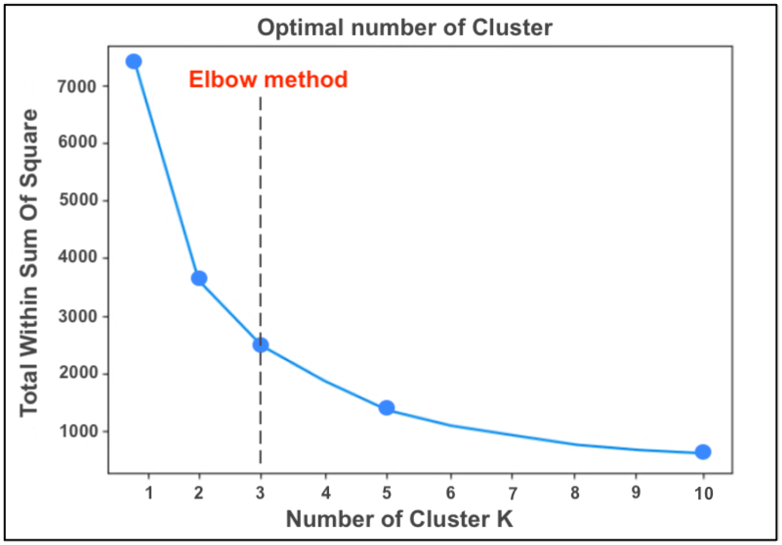
Based on the dataset provided, the algorithm applies the “elbow method” and returns, in output, the graph from which it is possible to extract the ideal number of Clusters to generate, equal to 3 (Figure 3).

This algorithm created 3 homogeneous clusters, characterized respectively by 10 (“cluster 0” in red), 29 (“cluster 1” in blue) and 16 (“cluster 2” in green) students (Figure 4).

In output, the graph represents the vectors associated with the different clusters on a two-dimensional plane of two of the 10 features used and the text containing the name of the grouping, followed by a list of numbers, in which each number identifies each student.

The results of K-Means are 3 clusters:

• Cluster 0: (4, 8, 12, 22, 25, 29, 30, 34, 43, 46)
• Cluster 1: (0, 1, 2, 3, 5, 6, 7, 10, 11, 14, 15, 21, 23, 24, 26, 27, 28, 31, 33, 35, 36, 38, 39, 40, 41, 45, 47, 51, 52)
• Cluster 2: (9, 13, 16, 17, 18, 19, 20, 32, 37, 42, 44, 48, 49, 50, 53, 54)

4.1.2. Mean-Shift

Mean-Shift was the second algorithm to be tested. The first step is to import the necessary libraries that Mean-Shift needs to perform the clustering process, then using scikit-learn’s Mean-Shift class, a Mean-Shift model was created easily, and we ran the algorithm using a bandwidth of 120. After running we can see the information for each feature. For example, let’s see the mean, standard deviation, minimum, and so on. Based on these values, the algorithm defines whether a student belongs to a specific cluster. In particular, we see that in cluster 0, we have 20 students, in cluster 1, there are 11 students, in cluster 2, there are 7 students, in cluster 3, there are 9 students and in cluster 4 there are 8 students.

The results of the Mean-Shift are 5 clusters

• Cluster 0: (1, 6, 7, 8, 9, 22, 23, 25, 29, 30, 33, 35, 36, 37, 41, 42, 43, 48, 49, 50)
• Cluster 1: (5, 10, 11, 12, 13, 14, 16, 26, 28, 31, 32)
• Cluster 2: (17, 24, 34, 38, 44, 52, 53)
• Cluster 3: (2, 3, 4, 20, 21, 40, 45, 51, 54)
• Cluster 4: (0, 15, 18, 19, 27, 39, 46, 47)

4.1.3. Agglomerative Clustering

After the Mean shift, Agglomerative Clustering was tested, using the scikit learn Agglomerative Clustering library. The algorithm generated a dendrogram in order to better visualize the clusters and to find the optimal number of clusters. Looking at the dendrogram (Figure 5), we can see that the highest vertical distance that doesn’t intersect with any clusters is the middle blue one. Given that 2 vertical lines cross the threshold, we can say that the optimal number of clusters is 2. So, seeing the dendrogram, we know that at the end we will have two groups of students.

The algorithm continues the execution with the creation of an instance of Agglomerative Clustering using the Euclidean distance as the measure of distance between points and also ward linkage in order to calculate the proximity of clusters.

The results of Agglomerative Clustering are 2 clusters:

• Cluster 0: (1, 6, 7, 8, 9, 17, 22, 23, 24, 25, 29, 30, 33, 34, 35, 36, 37, 38, 41, 42, 43, 44, 48, 49, 50, 52, 53)
• Cluster 1: (0, 2, 3, 4, 5, 10, 11, 12, 13, 14, 15, 16, 18, 19, 20, 21, 26, 27, 28, 31, 32, 39, 40, 45, 46, 47, 51, 54)

4.1.4. DBSCAN Clustering

DBSCAN clustering was another algorithm tested to create clusters of students. To use the algorithm, the scikit learn DBSCAN library was imported, setting by default the variable “epsilon” is equal to 67 and minimal number of samples are equal to 3, which is the minimum number of points that we need to create a cluster. We will store the labels that are formed by the DBSCAN algorithm and also the number of clusters that the algorithm has created by ignoring the noise if it is present. We can also see the noise using the variable “n_noise”.

The results of the DBSCAN are 5 clusters:

• Cluster 0: (1, 17, 24, 34, 38, 42, 44, 52, 53)
• Cluster 1: (0, 19, 39)
• Cluster 2: (6, 7, 8, 9, 22, 23, 25, 29, 30, 33, 35, 36, 37, 41, 43, 48, 49, 50)
• Cluster 3: (15, 18, 27, 46, 47)
• Cluster 4: (2, 3, 4, 5, 10, 11, 12, 13, 14, 16, 20, 21, 26, 28, 31, 32, 40, 45, 51, 54)

After the execution of the algorithm, we don’t have noise because the number of students in 5 clusters is the same as the initial number of students.

4.1.5. Gaussian Mixture Model

Then, using the Gaussian Mixture class of scikit-learn, we easily created a Gaussian Mixture Model and we performed the algorithm. After our model has converged, the weights, means, covariances and also the clusters are printed. The results of the “Means” are ((2.49090909e + 01 1.81818182e − 01 9.09090909e − 02 0.00000000e + 00...)), while the “Covariances” are (((3.96399174e + 03 2.01074380e + 01 1.03677686e + 01…))). Based on these results, 3 clusters will be created.

The results of Gaussian Mixture are:

• Cluster 1: (0, 2, 3, 4, 5, 10, 12, 14, 15, 16, 17, 18, 19, 20, 21, 24, 26, 27, 28, 31, 32, 38, 39, 40, 42, 46, 47, 54)
• Cluster 2: (1, 6, 7, 8, 9, 22, 23, 25, 29, 30, 33, 35, 36, 37, 41, 43, 48, 49, 50)
• Cluster 3: (11, 13, 34, 44, 45, 51, 52, 53)

4.1.6. Self-Organizing Map (SOM)

In order to implement the SOM algorithm, we used SOMPY, which is a Python Library. Next, It was initialized as a 20-by-20 Self-Organizing Map and it used the default parameters of SOMPY, like the initialization and neighborhood method. In Figure 6 we can see also a view of the clusters using the hitmap.

The results of SOM are 3 cluster:

• Cluster 0: (1, 6, 7, 8, 9, 10, 14, 22, 23, 25, 29, 30, 33, 35, 36, 37, 41, 42, 43, 48, 49, 50)
• Cluster 1: (0, 2, 3, 4, 12, 13, 15, 24, 27, 28, 31, 32, 38, 47, 52, 54)
• Cluster 2: (5, 11, 16, 17, 18, 19, 20, 21, 26, 34, 39, 40, 44, 45, 46, 51, 53)

4.2. Results of Clustering Algorithms

Silhouette Analysis

After running the different clustering algorithms, the Silhouette analysis method was run, used to interpret and validate the consistency within the data clusters. Using the result of each algorithm (generated clusters) and the data used to train the model, the silhouette score is calculated. The results of this analysis are displayed in the bar chart below (see Figure 7 for details).

As we can see from the plot above, the highest values are achieved from two algorithms: K-Means (a value of 0.644) and Mean Shift (with a value of 0.638). indeed, the algorithms that have the lowest values are Agglomerative Clustering and Gaussian Mixture Models Clustering, with a value of 0.54.

So, based on the theory of silhouette analysis and the results, the best algorithm is K-Means because it has the highest values among other algorithms with the value of 0.644.

4.3. Selection of the Best Clustering Algorithm and Development of the Software

After choosing the best clustering algorithm, the software was developed, and the K-means algorithm was inserted into it.

The clusters obtained by the software were then analyzed in order to determine the behaviors on the platform, highlighting which are the most influential features within the groupings. In this way, it is possible to profile the students who belong to a certain grouping.

As can be seen from

Table 1. Differences between clusters and details of the analyzed features.

	Cluster 0 Not Very Active Students on the Platform	Cluster 1 Students on Average Activity on the Platform	Cluster 2 Very Active Students on the Platform
n° students	10	29	16
n° access to the platform (average)	5.4	18.4	31.2
n°video tutorials viewed (average)	1.8	2.5	3
total viewing frequency of video tutorials (average)	7.4	11.2	16.2
n° video viewed (average)	2	4.1	4.3
total display frequency, of video experiments (average)	2.6	6.7	7
% students who completed the assignment	40%	90%	100%

, “cluster 0” represents the least active students on the platform, with a low number of accesses (average = 5.4), low frequency of views related to video tutorials (average = 7.4), and a low number and frequency of views related to the experiments (average = 2.6). The low participation is also reflected in the delivery of the individual paper, where only 40% of the students delivered the assignment on the platform.

“Cluster 1” represents students who are inactive or not too active in the platform. These users had an average of the number of accesses equal to 18.4, average of the number of video tutorials viewed equal to 2.5, average of the frequency of views of video tutorials equal to 11.2, average of the number of experiments viewed equal to 4.1, average of the viewing frequency of video experiments equal to 6.7. In this case, participation allowed 90% of students to carry out and deliver the final exercise. “Cluster 2” represents highly active students on the platform. These users had an average of the number of visits of 31.2, average of the number of video tutorials viewed equal to 3, and an average frequency of views of 16.2. The average number of experiments seen is 4.3 (5 total video experiments) while the average frequency of views is 7. This level of participation allowed all students to deliver the final paper (100% of the students).

To verify if the behavior carried out by students on the e-learning platform had feedback in terms of performance, we compared each cluster with the average of the marks for the individual work done by the students belonging to the same cluster. The results obtained are very interesting.

As reported in Figure 8, the level of participation in the platform of the students reflects the final grade. The most active students (“cluster 2”), in fact, received a higher score than the others with an average grade of 82.5. Students of “cluster 1”, with an average activity, had a lower rating with an average of 72.04, while students of “cluster 0” had an average grade, equal to 53. This strong correlation highlighted by the Pearson index equal to 0.986 allowed us to confirm the differences between the students belonging to the different clusters, not only in terms of behavior but also in terms of performance.

To demonstrate how student behavior affects the final student performance, ANOVA (analysis of variance) was used. ANOVA tests clusters of students grade to see if there is a difference between them [45].

A one-way ANOVA is used to test the null hypothesis that the means of multiple elements are all equal. Since after performing ANOVA, F > F crit (7.594799276 > 3.175140971), I reject the null hypothesis and accept the alternative hypothesis (at least one of the averages differs from the others). In fact, the average of the grades of the different clusters are significantly different from each other because the p value < alpha (0.001277126 < 0.05), which is the chosen significance level. Therefore, we claim that the averages of grades of the three clusters are not all the same; at least one of the means is different. Through post hoc controls (two sample t-tests) we compared the samples in pairs, in particular: (i) cluster 0 differs significantly from cluster 1 (p-value = 0.000152); (ii) the other two comparisons generated an insignificant p-value (cluster 0 vs cluster 1, p-value = 0.0201); and (iii) cluster 1 vs cluster 2, (p-value = 0.0517). We can conclude by stating that there is a significant difference between the three approaches above discussed. The approach with high activity (cluster 2) in the e-learning course differs significantly from that with low activity in the e-learning course (cluster 0). The approach with low activity (cluster 0) in the e-learning course is also different compared to that with average activity in the e-learning course (cluster 1).

Once the clusters were obtained, the software returned the creation of heterogeneous groups. We initially set the number of students for each group to 5, then the software ran.

The software applies the algorithm for creating heterogeneous groups, initially dividing the total number of students by 5, calculating how many heterogeneous groups you want to create. Then the number of students belonging to each group is calculated, by dividing the number of students in each cluster by the number of groups.

From Figure 9 we can see that once the algorithm was set, the software created 11 groups and automatically distributed the students in groups, so that in each group there was at least one student belonging to different clusters. In this way, it creates heterogeneous groups based on the behavior of the students.

Finally, the software automatically sent an e-mail to the teacher, with the list of heterogeneous groups, indicating the group name (e.g., group 0, group 1...) and next to each group the list of 5 numbers, the IDs that identify the students. In this way, the teacher was able to select students based on their ID, insert them into the relevant groups within Moodle and start the collaborative part of the course.

4.4. Moodle Plugin

Once the software was tested, it was also decided to turn it into a new Moodle plugin to help teachers creating heterogeneous groups.

It allows the loading of the dataset, which is the combination of two report files generated by the e-learning platform, and automatically creates heterogeneous groups.

Initially, the teacher enters his e-mail address, which is used by the plugin to send the email with the list of heterogeneous groups. The plugin then presents a button that allows the teacher to upload the excel files (Moodle Reports) downloaded from Moodle.

The files contain the features concerning the time, the behavior and the activities carried out by the students on the e-learning platform that represent the dataset that the machine learning algorithm will use for the creation of heterogeneous groups. This algorithm is activated thanks to the “Generate” button, which permits uploading files and performing clustering (see Figure 10 for details).

The Moodle plugin was developed using PHP as a programming language and also Python for the part of machine learning. So, after the user has uploaded the files and has clicked the submit button, the plugin will upload these files to a specific folder inside the plugin that is called “upload” (see Figure 11 for details).

Then, the plugin gets these excel files, merges them and generates an excel file called “merge.excel”, which is the input dataset file. This file will be placed in the same directory where the excel files are uploaded from the user. Then the machine learning algorithm gets the dataset file and performs the clustering process. Then the result of the algorithm, which is a string with the groups created, will be displayed to the teacher and also sent to the teacher email (See Figure 12 for details).

5. Conclusions and Future Developments

In this work, we have designed and created a new algorithm and corresponding software aimed at helping teachers in defining groups of students for collaborative activities. Machine Learning techniques have allowed us to demonstrate how these help to improve the creation of heterogeneous groups of students. The ability to test the efficiency and performance of the clustering algorithms was important in choosing the best one, in order to better analyze the characteristics for each cluster by delineating different student profiles accurately.

The comparison between the clusters obtained and the average of the final grade of the students of each cluster confirmed the differences between the clusters also in terms of performance. The most active students (“cluster 2”) received a higher score than the others with an average grade of 82.5. Students of “cluster 1”, with an average activity, had a lower rating with average of 72.04, while the students of “cluster 0” with low activity in the platform had an average grade equal to 53.

By applying these techniques to the collected data and verifying the efficiency of the techniques, it was possible to guarantee and maximize the heterogeneity of the students within each group. This increases the chances of success for all students in group works within the online course.

The Learning Analytics of the Moodle e-learning platform has been taken as a feature so that the software realized in this work can be reused by other teachers and tutors who carry out online teaching activities on Moodle. The choice of the Moodle platform is not binding for the execution of our software, because it is easily adaptable to any other LMS (Learning Management System), by modifying the dataset.

At the end of this experiment with the Physics Laboratory online course, which will still need several months to be concluded, we will be able to test if the use of the heterogeneous groups could improve the students’ perceptions regarding the peers’ feedbacks. It could be interesting also to analyze the final grades of the students after peer review to check if there will be a uniform improvement compared to the past.

Future developments of our work will consist of realizing additional applications of the new Moodle plugin described in this work. To compare how our approach will perform on different disciplines, we will use our software on the Genomics course, where peer review has been applied in the past using only random groups.