Analysis of Seismic Wavefield Characteristics in 3D Tunnel Models Based on the 3D Staggered-Grid Finite-Difference Scheme in the Cylindrical Coordinate System

Abstract

The accurate prediction of the geological conditions ahead of a tunnel plays an important role in tunnel construction. Among all forward geological prospecting methods, the seismic detection method is widely applied. However, due to the characteristics of the tunnel and the complexity of the geological conditions, the seismic wavefield is complicated. Carrying out a more realistic forward modeling method is vital for fully understanding the law of seismic wave propagation and the characteristics of seismic wavefield in the tunnel. In this paper, the 3D staggered-grid finite-difference scheme in the cylindrical coordinate system based on the decoupled nonconversion elastic wave equation is used to carry out the numerical simulation. This method can avoid the diffraction interferences produced at the edges of the tunnel face in the Cartesian coordinate system. Based on this forward modeling method, the characteristics of wavefield and propagation laws of seismic waves under three kinds of common typical unfavorable geological models were explored, which can provide theoretical guidance to seismic data interpretation of tunnel seismic forward prospecting in practice.

1. Introduction

The accurate prediction of the geological conditions in front of the tunnel during construction is critical. The tunnel seismic forward prospecting is one of the mainstream methods in the current tunnel forward geological prospecting [1]. By projecting seismic waves on the sidewall or face of the tunnel, the seismic waves propagate around and produce reflection, transmission, multiple reflections, etc. at the geological interfaces, which are subsequently received by the receivers arranged on the tunnel. By data processing methods, such as migration and inversion methods, the geological conditions in front of the tunnel can be obtained. However, due to the geological interfaces caused by excavation between the tunnel cavity and the surrounding rock, and the complex geological conditions in front of the tunnel, the seismic wavefield is complex, which leads to difficulty of the interpretation of seismic data. Therefore, it is of great significance to study the characteristics of seismic wavefield and propagation laws under different unfavorable geological conditions.

Wavefield analysis is important to research in that it is helpful for the reasonable arrangement of observation devices, understanding of seismic data, and accurate interpretation of seismic data. Researchers have analyzed seismic wavefields and propagation based on numerical modeling or experiments to help in the field of seismic exploration. Sanchez-Salinero et al. [2] carried out the analytical studies of body wave propagation and attenuation and gave a better field setup that helps to reduce the detrimental effects of near-field waves. To better obtain the formation of shear velocity, Joongmoo Byun et al. [3] analyzed the acoustic wavefields projected by logging-while-drilling. Raji et al. [4] study the characteristics of the wavefield of crosswell seismic data. The seismic wave propagation cross rock mass has been investigated by Fu et al. [5] and Li et al. [6]. In the oil–gas exploration field, the characteristic of seismic wavefield in fractured media has been studied [7,8,9]. In the field of tunnel construction, Wang et al. [10] studied the seismic wave propagation patterns around mine tunnels for dynamic rock support. Liu et al. [11] studied the seismic response characteristics of the crossing tunnels through experiments and numerical modeling.

Among the seismic forward modeling methods, the finite-difference modeling method in the Cartesian coordinate system is the mainstream. Alterman et al. [12] used the finite-difference method to simulate the propagation of elastic waves for the first time. Subsequently, the staggered-grid finite-difference scheme in 2D [13] and 3D have been developed [14].

However, there are unavoidable problems in the finite-difference scheme in the Cartesian coordinate system. Because the mesh grid adopts a square grid, the surface of the tunnel, which usually is cylindrical, cannot be accurately divided. Furthermore, when seismic waves pass through the tunnel face, there will be many strong diffraction waves produced at the edges of the tunnel face, which will disturb the actual seismic wave field.

Considering that the tunnel is a cylindrical cavity, the finite-difference scheme in the cylindrical coordinate system is a more suitable way to simulate seismic wavefield and study its characteristics in the tunnel. Some related studies have shown its effectiveness. In electromagnetic forward modeling, the finite-difference scheme in the cylindrical coordinate system is widely used to simulate the propagation of electromagnetic waves in cylindrical objects [15,16] and has shown that it outperforms. In the seismic forward modeling, Liu [17] performed elastic wave forward modeling in cylindrical coordinates to simulate the propagation of elastic waves in sonic logging, but the algorithm uses pseudo-3D equations, which essentially operate in two dimensions. Pissarenko et al. [18] realized the finite-difference simulation of sonic logging using the cylindrical coordinate system. Toyokuni et al. [19] and the other Japanese scholars carried out research on local or global seismic forward modeling and deduced elastic wave equations in cylindrical and spherical coordinate systems. Recently, Liu et al. studied the 3D dispersion features of the velocity and ellipticity of the Rayleigh wave in the cylindrical coordinate system. Luo et al. [20] used the cylindrical coordinate system finite-difference algorithm to simulate the seismic wave propagation in the tunnel space for the first time, especially for the situation where the front is rich in karst caves. However, the study also regarded the tunnel space as an axisymmetric problem. The 3D problem was simplified to a 2D.

Therefore, in order to better study the characteristics of seismic wavefield in front of tunnel, it is necessary to carry out the research of seismic forward modeling method based on a 3D cylindrical coordinate system. In this work, considering the compatibility between tunnel shape and cylindrical coordinates and its better simulation precision, numerical simulation is carried out under the three kinds of unfavorable geological conditions in tunnel construction based on the finite-difference scheme of 3D uncoupled nonconverted elastic wave equation in the cylindrical coordinate system. Through the numerical experiments and analysis, some significant conclusions are drawn. This forward method could be used to simulate and analyze the wavefield characteristics for vertical seismic profiling (VSP) in 3D to help researchers understand the seismic wavefield propagation in the geothermal area.

2. Methods

To analyze the characteristics of wavefield and its propagation more accurately, we adopt a finite-difference scheme of 3D the decoupled nonconversion elastic wave equation in the whole space of the tunnel based on the cylindrical coordinate system. The 3D decoupled nonconversion elastic wave equation will be introduced briefly.

2.1. The 3D Decoupled Nonconversion Elastic Wave Equation in the Cylindrical Coordinate System

In a 3D homogeneous medium, the time-domain elastic wave equation in Cartesian coordinates [21] can be expressed as:

$$\rho \frac{{\partial }^2\mathit{u}}{\partial t^2}=(\lambda +\mu )\nabla \nabla ·\mathit{u}+\mu {\nabla }^2\mathit{u}-\nabla \lambda \nabla ·\mathit{u}+\nabla \mu \times (\nabla \times \mathit{u})+2(\nabla \mu ·\nabla )\mathit{u},$$

(1)

where $\mathit{u}$ is the displacement of the elastic wavefield, $\rho$ denotes the density, t is the time, and $\mu ,\lambda$ represent Lame constants, respectively. Yao [22] multiplied the above equation by $\nabla ·$ or $\nabla \times$ and brought the nonconversion condition into it, obtaining the nonconversion elastic wave equation as follows:

$$\frac{{\partial }^2\mathit{u}}{\partial t^2}=\nabla (v_P^2\nabla ·\mathit{u})-v_S^2\nabla \times \nabla \times \mathit{u},$$

(2)

where $v_S$, $v_P$ denote the P-velocity and S-velocity, respectively. According to the Helmholtz theory, we can decouple the S-wavefield and the P-wavefield and obtain Equation (3),

$$\left\{\begin{array}{c}\mathit{u}={\mathit{u}}^P+{\mathit{u}}^S,\hfill \\ {\displaystyle \frac{{\partial }^2{\mathit{u}}^P}{\partial t^2}}=\nabla \left(v_P^2\nabla ·\mathit{u}\right),\hfill \\ {\displaystyle \frac{{\partial }^2{\mathit{u}}^S}{\partial t^2}}=v_S^2\nabla \times \nabla \times \mathit{u},\hfill \end{array}\right.$$

(3)

where ${\mathit{u}}^P$, ${\mathit{u}}^S$ are the displacement of P-wavefield and S-wavefield, respectively. By introducing the stress field and defining the particle vibration velocity, the first-order velocity–stress equation for the decoupled nonconversion elastic wave in cylinder coordinates can be expressed as:

$$\left\{\begin{array}{c}{v}_r=v_r^P+v_r^S,{\displaystyle \frac{\partial v_r^P}{\partial t}}={\displaystyle \frac{\partial {\tau }^P}{\partial r}},{\displaystyle \frac{\partial v_r^S}{\partial t}}={\displaystyle \frac{\partial {\tau }_{zr}^S}{\partial z}}-{\displaystyle \frac{\partial {\tau }_{r\theta }^S}{r\partial \theta }},\hfill \\ v_{\theta }=v_{\theta }^P+v_{\theta }^S,{\displaystyle \frac{\partial v_{\theta }^P}{\partial t}}={\displaystyle \frac{\partial {\tau }^P}{r\partial \theta }},{\displaystyle \frac{\partial v_{\theta }^S}{\partial t}}={\displaystyle \frac{\partial {\tau }_{r\theta }^S}{\partial r}}-{\displaystyle \frac{\partial {\tau }_{\theta z}^S}{\partial z}},\hfill \\ v_z=v_z^P+v_z^S,{\displaystyle \frac{\partial v_z^P}{\partial t}}={\displaystyle \frac{\partial {\tau }^P}{\partial z}},{\displaystyle \frac{\partial v_z^S}{\partial t}}={\displaystyle \frac{\partial {\tau }_{\theta z}^S}{r\partial \theta }}-{\displaystyle \frac{\partial \left(r{\tau }_{zr}^S\right)}{r\partial r}},\hfill \\ {\displaystyle \frac{\partial {\tau }^P}{\partial t}}=v_P^2\left({\displaystyle \frac{\partial v_r}{\partial r}}+{\displaystyle \frac{v_r}{r}}+{\displaystyle \frac{1}{r}}{\displaystyle \frac{\partial v_{\theta }}{\partial \theta }}+{\displaystyle \frac{\partial v_z}{\partial z}}\right),\hfill \\ {\displaystyle \frac{\partial {\tau }_{r\theta }^S}{\partial t}}=v_S^2\left({\displaystyle \frac{\partial \left(r{v}_{\theta }\right)}{r\partial r}}-{\displaystyle \frac{1}{r}}{\displaystyle \frac{\partial v_r}{r\partial \theta }}\right),\hfill \\ {\displaystyle \frac{\partial {\tau }_{\theta z}^S}{\partial t}}=v_S^2\left({\displaystyle \frac{\partial \left(v_z\right)}{r\partial \theta }}-{\displaystyle \frac{\partial v_{\theta }}{\partial z}}\right),\hfill \\ {\displaystyle \frac{\partial {\tau }_{zr}^S}{\partial t}}=v_S^2\left({\displaystyle \frac{\partial \left(v_r\right)}{\partial z}}-{\displaystyle \frac{\partial v_z}{\partial r}}\right),\hfill \end{array}\right.$$

(4)

where ${\tau }_{ij}^S,{\tau }_{ij}^P(i,j\in [r,\theta ,z])$ are the stress field component of the P-wavefield and S-wavefield, respectively. $v_i(i\in [r,\theta ,z])$ denotes the particle vibration velocity component, and $r,\theta ,z$ are the spatial directions in the cylindrical coordinate system.

2.2. Stability Conditions and Absorbing Boundary Conditions

The stability condition and absorbing boundary condition of the finite-difference scheme are two important aspects. The stability condition is a restrictive condition given for the numerical dispersion problem in the simulation process, and the absorbing boundary condition is used to absorb and suppress the reflected wave generated by the artificial boundary.

Liu et al. [23] derivated the 3D elastic wave equation in the cylindrical coordinate system and pointed out that the finite-difference stability conditions in the cylindrical coordinate system are more strict than that in the Cartesian coordinate system. This is because the meshing method is still following that under the Cartesian coordinate system. When the number of meshes is fixed, frequency dispersion will occur until the length of the mesh element in the direction will gradually increase to the limitation of stability condition with the increases of radius. Therefore, to maintain the stability of the calculation and avoid numerical dispersion, the only way is to sacrifice the amount of calculation. To solve the above problems, we can possibly adopt a variable grid method instead, gradually increasing the number of grid divisions as the radius increases, so that the length of the division element in the direction is always under the stability condition in the Cartesian coordinate system as shown in the following formula, which can save the amount of calculation as much as possible while avoiding the numerical dispersion.

$$\left\{\begin{array}{c}\Delta r,{\displaystyle \frac{2\pi i\Delta r}{N}},\Delta z\le {\displaystyle \frac{{\lambda }_{min}}{6}}\hfill \\ \Delta t\le {\displaystyle \frac{min\left(\Delta r,{\displaystyle \frac{2\pi i\Delta r}{N}},\Delta z\right)}{\sqrt{3}{v}_{max}}}\hfill \end{array}\right.(i=1,2,3\cdots )$$

(5)

Among them, $\Delta r,\Delta z$ are the minimum grid length in space, i is the number of divisions in the r direction, N denotes the number of meshing elements in the $\theta$ direction, $\Delta t$ is the sampling time interval, and $v_{max}$ represents the maximum wave velocity.

Because forward modeling is only performed in a limited area, artificial boundaries will be formed around the area. When seismic waves propagate to the boundary, reflections will occur, which will interfere with the original wavefield and cause boundary problems. Aiming at this problem, we adopt the elastic wave PML absorption boundary in the cylindrical coordinate system proposed by Liu [23].

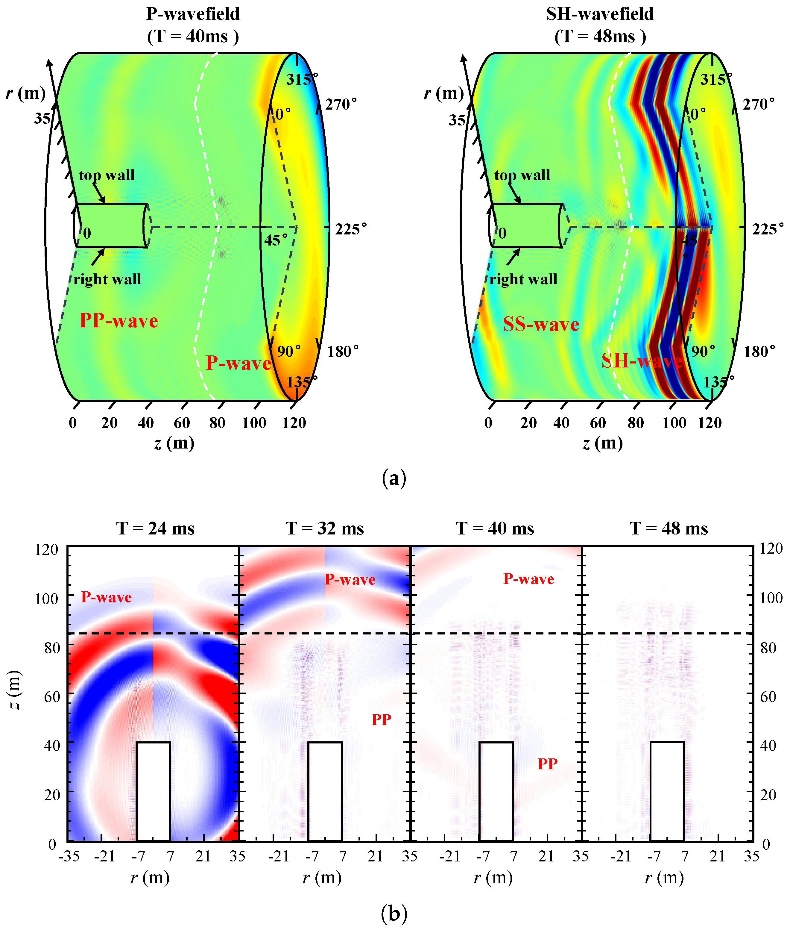
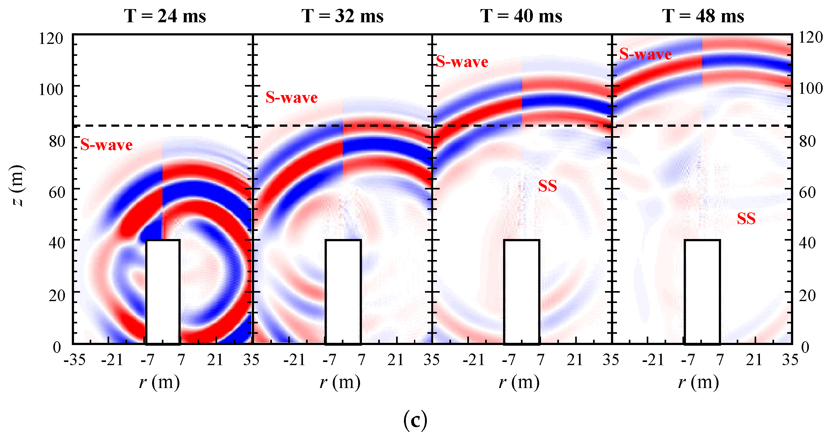
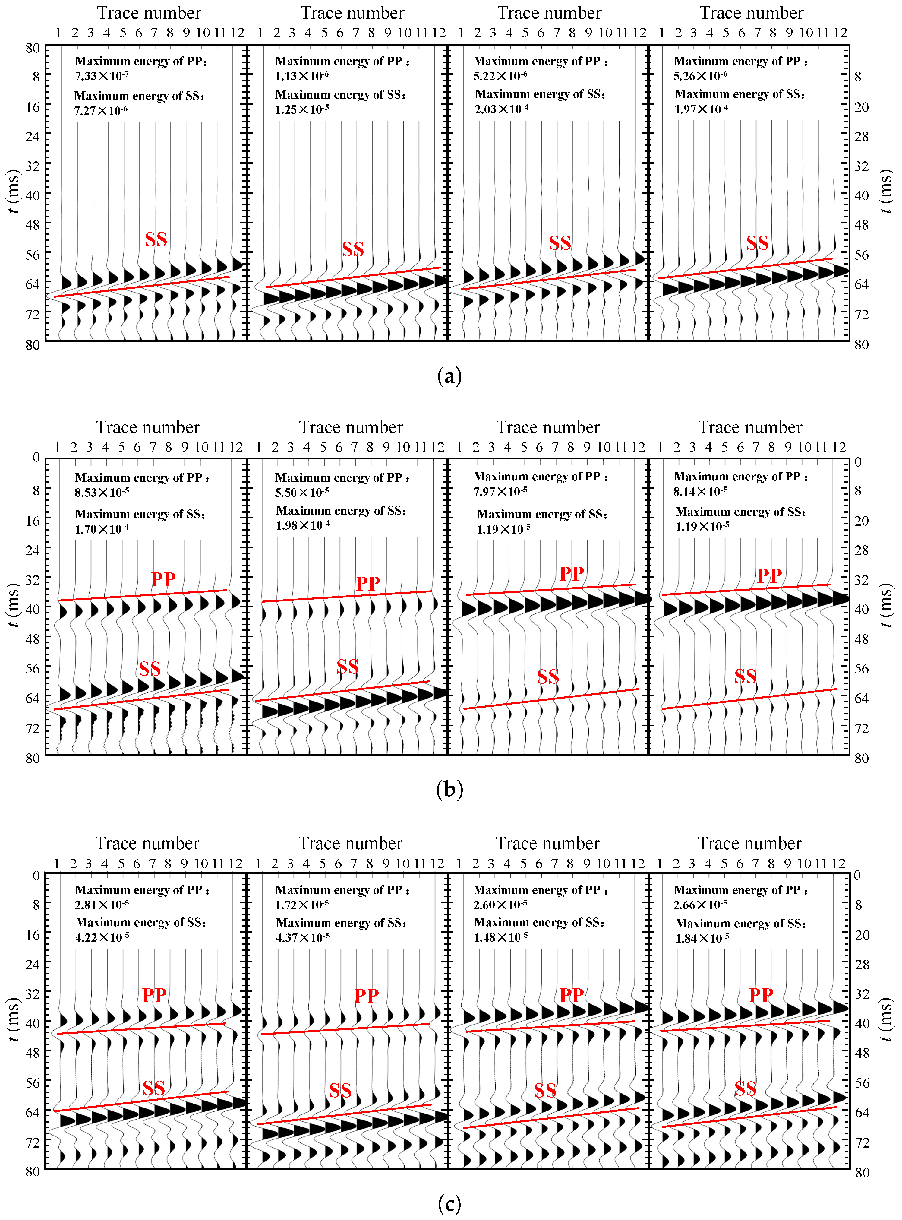
3. Numerical Experiment

For the convenience of analysis, we will use the same observation system. The specific parameters are shown as follows. The seismic source is arranged on the right wall of the tunnel, 12 m away from the tunnel face, and the dominant frequency is 100 Hz. There are two survey lines, which form a space observation system. The first survey line is arranged on the left and right sidewalls of the tunnel. The nearest receiver is 18 m away from the tunnel face. The receivers are separated by 2 m. There are 12 on the left and right sidewalls, respectively. The other survey line is symmetrically arranged on the upper and lower sidewalls of the tunnel, and the nearest receiver is 13 m away from the tunnel face, the number of which is equal to survey line 1.

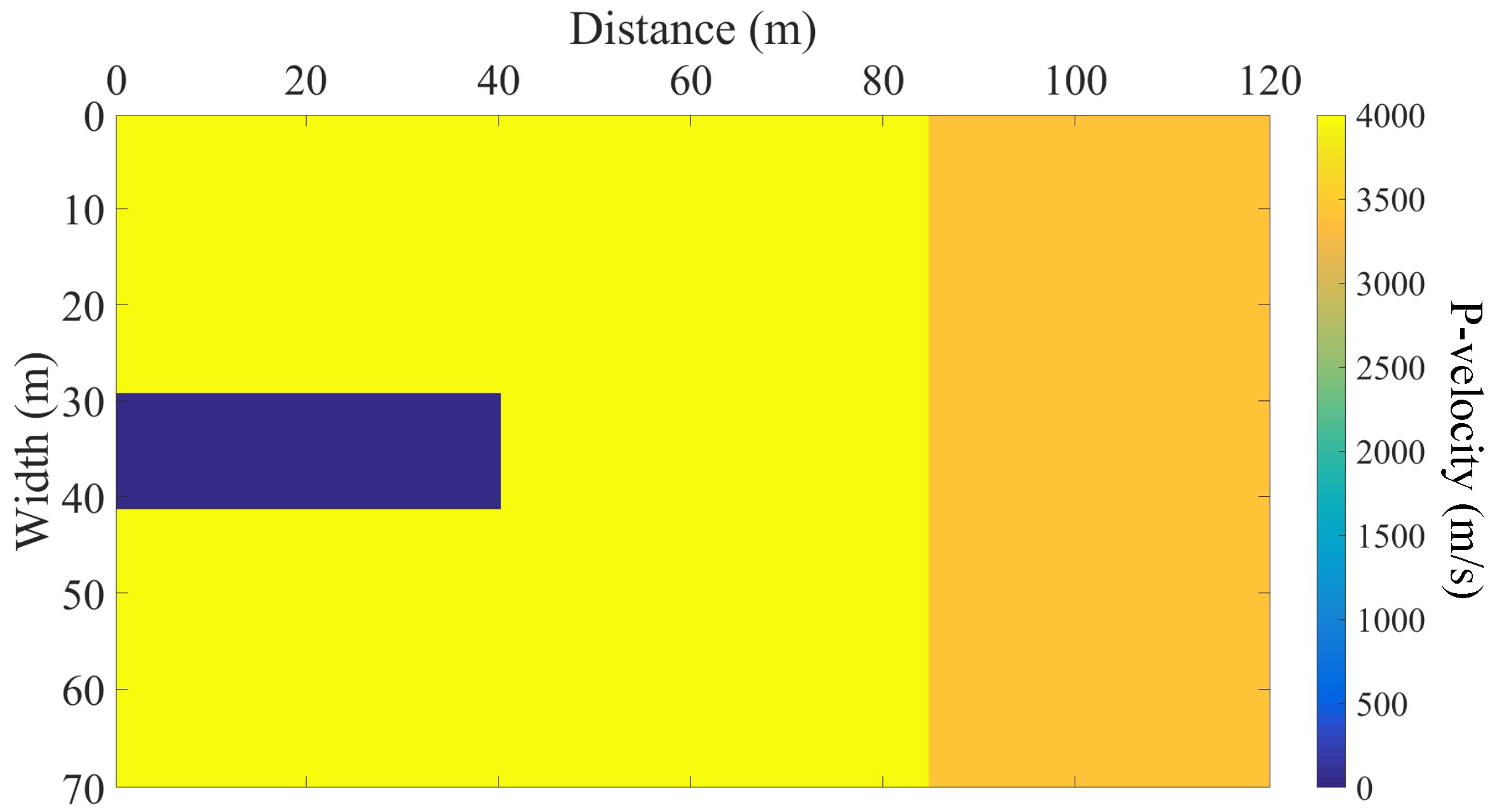
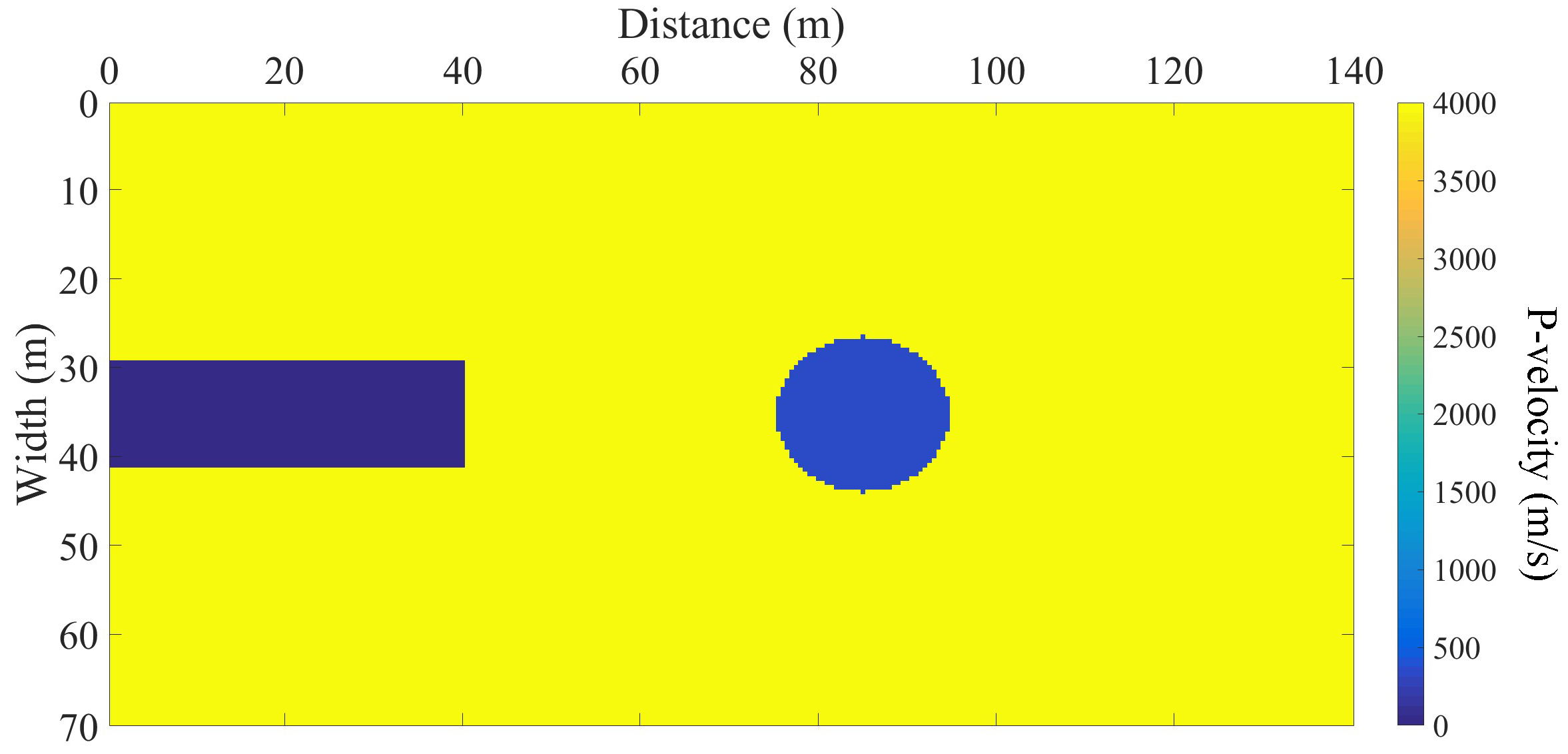
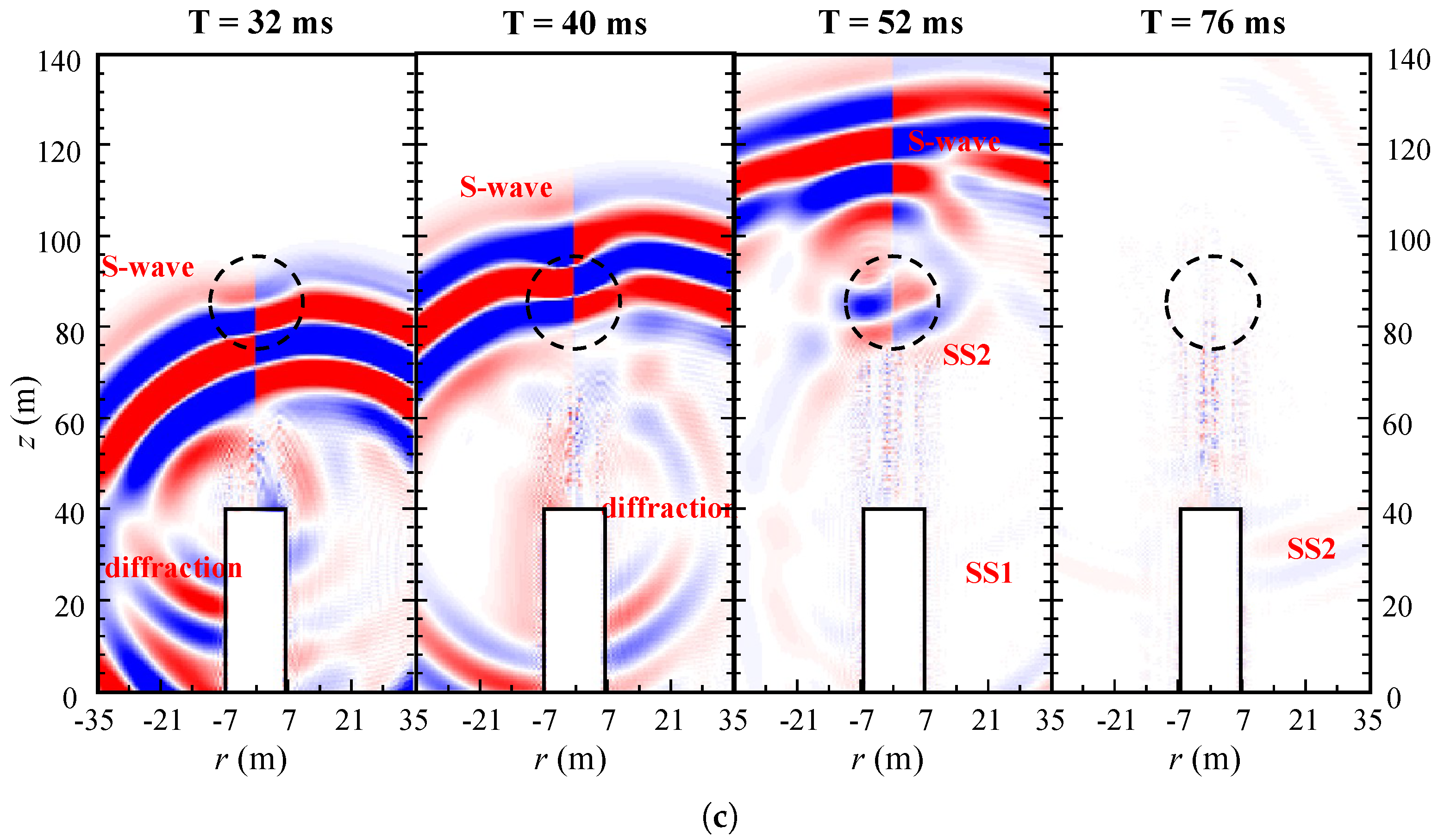
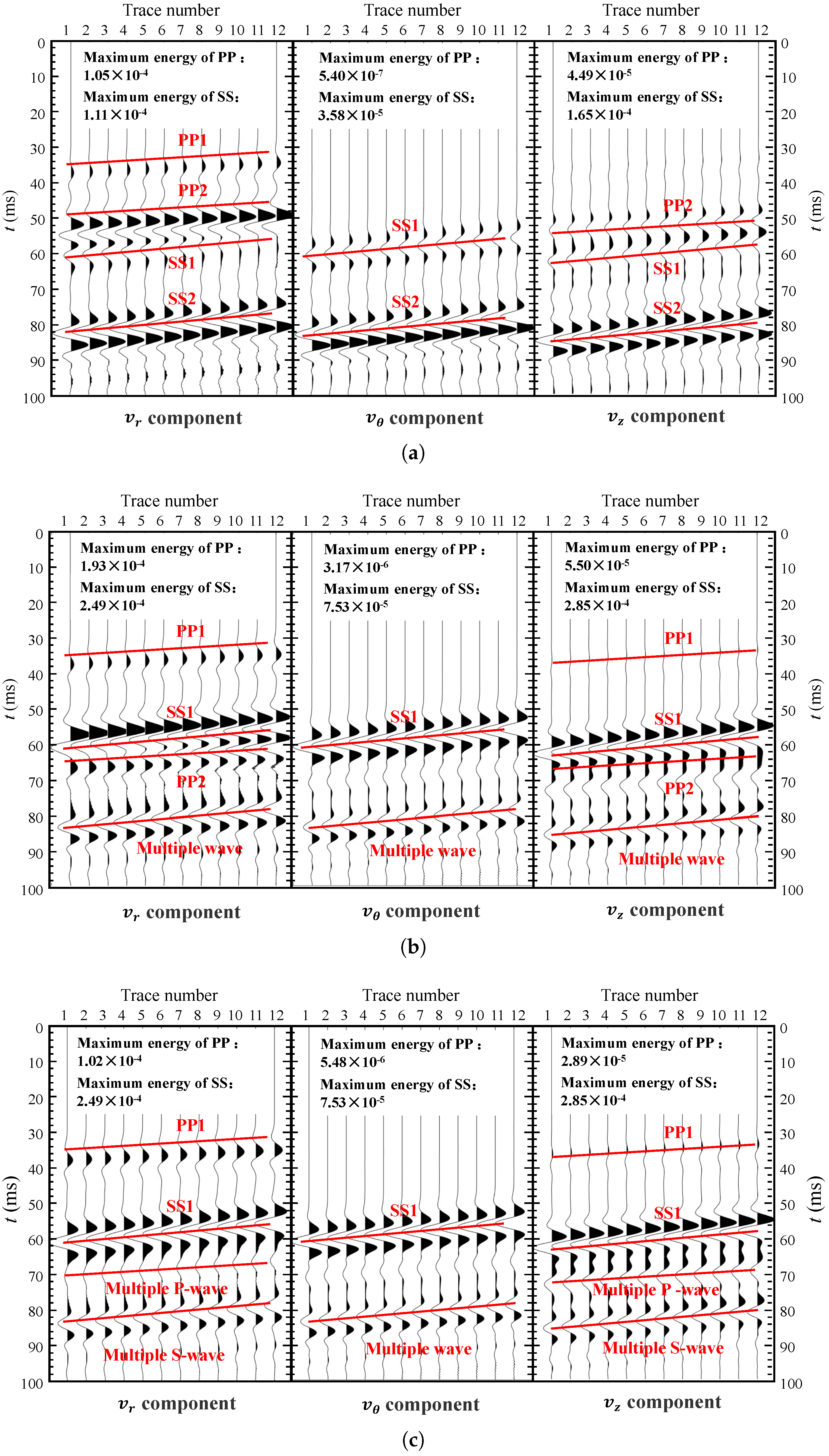
3.1. Single Vertical Geological Interface Model

As shown in Figure 1, we set up a model with a single vertical geological interface and its radius and width are 35 m and 120 m, respectively. The tunnel is 40 m long and has a radius of 6 m. The center of the interface is 45 m away from the tunnel face in the z-direction. The P-velocity and S-velocity of the surrounding rock are $V_P=4000$ m/s and $V_S=2300$ m/s, respectively; those of the medium behind the interface are $V_P=3400$ m/s and $V_S=2000$ m/s; the grid spacing is $\Delta r=\Delta z=0.5$ m. The time sampling interval is $0.2$ ms, and the total time window is $0.08$ s.

In Figure 2a, it can be seen that this method can simulate the propagation process of the tunnel full-space seismic wavefield well and separate the P-wave and S-wave fields. Since the source is put on the sidewall, the energy of S-waves is stronger than that of P-waves. It can be seen from Figure 2b,c that the direct P-wave reaches the reflector at about 24 ms, the reflected $PP$-wave was collected by receivers at 40 ms, and the direct S-wave reaches the reflector at 32 ms. The reflected $SS$-wave is received at 56 ms.

As for the seismic profiles, the direct wave has been removed from all of the seismic data shown in the figure to prevent it from affecting reflected waves. Figure 3a is a three-component seismic profile of a single-layer vertical interface on each survey line. First, the shear waves mainly propagate along the z and r directions, so the energy of the reflected waves in the $v_{\theta }$ component is weak, and S-waves are the main ones. The P-wave mainly propagates along the r direction in the $roz$ plane. The energy of the reflected P-wave in the $v_r$ component is the strongest, followed by that in the $v_z$ component, and the energy of the reflected P-wave in the $v_{\theta }$ component seismic profile is the weakest. Then, let us compare the difference between the reflected waves of each survey line, analyze the amplitude energy characteristics of the event axis of the reflected wave, and remove the $v_{\theta }$ component. Two laws can be summarized: ① In the seismic profile from the left and right sidewall, the energy of the S-wave is stronger than the P-wave. However, in that of upper and lower sidewalls, that is opposite. ② The energy of the reflected P-wave from the right wall is stronger than that from the left side wall, and the same observation can be made for the reflected S-wave energy. In summary, in the three-dimensional tunnel space, different components and different survey lines can receive different reflected wave information. Therefore, in tunnel forward seismic prospecting, the seismic data from multicomponent and multisurvey lines should be used comprehensively.

As shown in Figure 4, the karst cave model is a cylindrical space with a radius of 35 m and a height of 140 m. The karst cave has a diameter of 20 m and a distance of 45 m in front of the tunnel face. It is filled with three media: water, soft soil, and air, respectively. The sampling interval is $0.2$ ms, and the total calculation time is $0.1$ s.

The specific physical parameters of the filling medium in the karst cave are shown in

Table 1. Physical parameters of the different mediums in the karst cave model.

Medium	$\mathit{\rho }$ (kg/m${}^3$)	${\mathit{V}}_{\mathit{P}}$ (m/s)	${\mathit{V}}_{\mathit{S}}$ (m/s)
Surrounding rock	2000	4000	2300
Soft soil	1800	2500	1700
Water	1000	1500	0
Air	1.0	340	0

.

We select the snapshot of the 3D wavefield of the karst cave model filled with soft soil and its slice diagram for demonstration. It can be seen from Figure 5 that the seismic wave reflects for the first time when it passes through the first interface of the karst cave and then spreads in the spherical form with the cave as the center. The other part passes through the cave space in the form of a transmission wave, which produces diffraction inside the cavity, and finally, a second reflected wave is transmitted back to the receivers. As shown in Figure 6b, the first P-wave reflection $PP1$ reaches the tunnel face at 32 ms, and the second reflection P-wave $PP2$ formed after diffraction is formed at 40 ms and is received by the receivers at 52 ms. Similarly, the two reflected waves $SS1$ and $SS2$ of S-wave arrive at the survey line at 52 ms and 76 ms, respectively. The diffracted waves on the tunnel face can be observed in the transverse wave field, which shows that although the method can avoid the interference of the diffracted waves at the edges of the tunnel face emerging in the Cartesian coordinate system, it cannot suppress the diffracted waves generated at the junction of the surface edge and the sidewall.

When the cave is filled with other media, the basic characteristics of the seismic wavefield are similar to those of soft soil. The main difference lies in the energy intensity of the reflected waves and whether the P/S-waves can pass through the cave space. In the following, we will further compare the three-component seismic profiles of survey line 1 when the cave is filled with different media.

Figure 6a shows the three-component seismic profile when the karst cave is filled with soft soil. Similar to the model with a vertical single interface, the energy of the S-wave is still stronger than that of the P-wave. In the seismic profile of the $v_z$ component, the energy of $PP1$ is relatively weak and almost unrecognizable, whereas in the seismic profile of the $v_{\theta }$ component, only the reflected S-wave can still be observed. The energy of the reflected P-wave is the strongest in the seismic profile of the $v_r$ component, and the energy of the reflected S-wave is the strongest in the seismic profile of the $v_z$ component. Comparing the energy of the two kinds of reflected waves, it can be found that the energy of the second reflected waves is stronger than that of the first. This is mainly because the first interface of the cave has a “divergence” effect for the seismic wave. This interface and the inside of the cavernous cavity play the role of “gathering” seismic waves.

Figure 6b is the seismic profile obtained under a water-filled karst cave. Same as the aforementioned result, the energy of the reflected P-wave is still the strongest in the seismic profile of the $v_r$ component and the energy of the reflected S-wave is strongest in the seismic profile of the $v_z$ component. However, in the $v_{\theta }$ component, the energy of the reflected waves is weakest. This is different from the observation of that under a soft-filled karst cave, mainly in the value of maximum energy of the reflected P-wave and S-wave and the waveform of the reflected S-wave. From the perspective of the energy of the reflected wave, the enegry of the reflected wave is different for the difference of the reflection coefficient of media. When the surrounding rock conditions are the same, the P-wave reflection coefficient between surrounding rock and water is larger, and the reflection coefficient of the S-wave is much larger than that of the soft soil medium. Therefore, the energy of reflected P-/S-waves increases greatly. From the perspective of the waveform, the P-wave can pass through the cave, and the second reflected P-wave is formed at the interface behind the karst cave. The energy of $PP2$ is stronger than that of $PP1$. However, since the propagation of the P-wave inside the karst cave, the first arrival time of $PP2$ is later than that of $SS1$. The S-wave cannot propagate across the water, so the second reflected S-wave $SS2$ will not be formed. However, there is an in-phase axis can be observed after $SS1$ from the seismic profile, but the energy is much smaller than $SS1$. Comparing the snapshot of the wavefield, it can be concluded that this event axis is the multiple waves generated by the S-wave.

Figure 6c is the seismic profile of a karst cave filled with air. Because the S-wave velocity in the air is the same as that in the water, the energy intensity and first arrival time of the S-wave reflection are the same as that in Figure 6b. The main differences lie in the reflection of P-waves: the P-velocity in the air (acoustic wave) is much lower than that in other media. Therefore, it can be approximated that P-waves cannot pass through the cavity to form $PP2$. This is why only the in-phase axis of $PP1$ can be observed in Figure 6c. As for the energy of P-wave reflection, from a numerical point of view, although the maximum energy of the P-wave is reduced, it is the energy of $PP1$, which is close to that of $PP2$ enhanced by the focusing effect of karst cavity filled with soft soil. It can be determined that the energy of the reflected wave produced by the cavity is the strongest, which also explains the strong interference of the tunnel body to the seismic wavefield. Since the caves and tunnels are strong reflectors at this time, the energy of reflected waves is enhanced, and the energy of multiple waves is also greatly enhanced. Therefore, the multiple waves generated by P/S-waves can be observed in the seismic profile of Figure 6c.

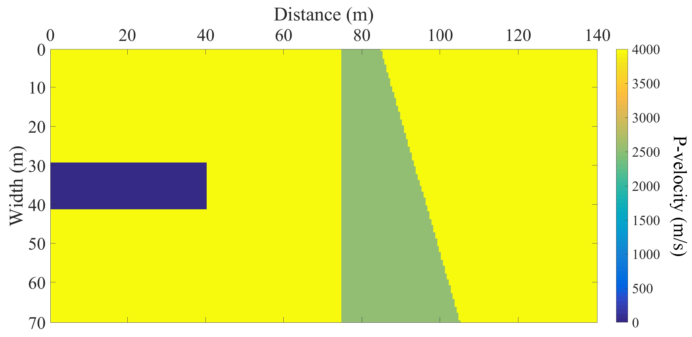
3.2. Wedge-Shaped Fault Model

As shown in Figure 7, a wedge-shaped fault model with a wide top and a narrow bottom is set up, with a radius of 35 m and a length of 140 m. The front interface of the fault is vertical, 35 m away from the tunnel face, the rear interface is inclined with a dip angle of ${70}^{\circ }$, the widest part of the upper part at the fault is 30 m, and the narrowest part at the lower part is 10 m. The fault is filled with soft soil. The rest of the model settings are the same as those used in the karst.

From Figure 8, it can be seen that the wedge-shaped fault model also produces reflected waves twice. $PP1$ reaches the receivers at 32 ms and $SS1$ is received at 48 ms. The first reflected wave is completely vertical, whereas the second reflected waves are inclined, and there is a certain time difference when they reach the upper and lower sidewall. When the dominant frequency of the source remains constant, because the P-wave velocity is larger, the wavelength of the reflected P-wave is greater than the that of reflected S-wave, so the resolution of the S-wave is higher, and it is more suitable for detecting small-scale structures.

For simplicity, only the seismic profile from the upper and lower sidewalls in $v_r$ component will be illustrated. As shown in Figure 9, comparing the P-waveform and S-waveform in the seismic profiles of the upper and lower sidewalls, the following differences can be summarized: (1) In the wedge model, the first interface is vertical and the second interface is tilted, causing the reflection waves $PP1$ and $SS1$ generated by the first interface to be the same when they arrive at the upper and lower sidewalls. The second reflection waves $PP2$ and $SS2$ in the upper wall survey line arrives later than that from the lower sidewall, and the time delay of the S-wave is more obvious; (2) Since the first interface of the wedge model is closer to the tunnel face, the energy of reflected waves is stronger than that in aforementioned model with a single-reflective interface; (3) The energy of reflected waves in the seismic profile from the lower sidewall is greater than that from the upper sidewall; (4) The energy of $PP2$ is less than that of $PP1$. The energy of $SS2$ is slightly larger than that of $SS1$. When the interface inclination angle is large, the S-wave is less affected by the change of inclination angle, and the reflected S-wave energy gradually increases as the inclination angle decreases. However, the P-wave is greatly affected by the change of the inclination angle, the energy of the reflected P-wave will decrease first, and the decrease on the survey line on upper sidewall is more obvious.

4. Discussion

In order to verify the effectiveness of the proposed method in this paper, we compared it with the 3D staggered-grid finite-difference scheme in the Cartesian coordinate system. In order to show the advantages of this method, we use the 3D elastic wave equation to simulate the wave field propagation ahead of the tunnel.

Take the model setting in the Cartesian coordinate system as an example (the model size and observation setup setting in the cylindrical coordinate system are exactly the same); the model size is $40\times 40\times 140$ m, the size of grid is $0.5$ m. The tunnel is 30 m long and has a width (diameter) of 12 m. In terms of observation methods, a source is set at the center point of the top of the tunnel, 5 m from the tunnel face, and the main frequency is 120 Hz. There are two survey lines. Survey line 1 is set on the face of the tunnel, around the tunnel; survey line 2 is set 20 m to 50 m in front of the tunnel, arranged along the z axis, with an interval of 1 m, totally 31. In addition to the air medium in the tunnel area, the surrounding rock area is set as a homogeneous medium, with $V_p=4000$ m/s and $V_s=2300$ m/s.

Comparing the wavefield results in $ro\theta$ plane in Cartesian coordinate system and cylindrical coordinate system, it can be seen that the interference of diffracted waves is mainly caused by $SH$-waves, which detour along the tunnel boundary during the propagation process. When the seismic wave meets the mutation point (indicated by the red dots in Figure 10), a strong diffraction wave will be generated. In the cylindrical coordinate system, the wave fields is clean. However, because the S-wave can propagating along the two sides of the tunnel meet each other at the bottom of the tunnel, there will be a slight dispersion phenomenon (shown by the arrow in Figure 10).

Further comparing the seismic profiles of survey line 1 and survey line 2, as shown in Figure 11, it can also be seen that the forward simulation method in cylindrical coordinates is significantly better than that in the Cartesian coordinate system in suppressing the interference of diffracted waves at the mutation point. Because survey line 1 is arranged around the tunnel, the seismic profileing event axis presents a typical “X” shape. The intersection of the event axis corresponds to the receiver at the bottom of the tunnel. Therefore, the dispersion caused by the interference of seismic waves is only generated in the lower half of the “X” shape. The frequency is higher than the direct wave, and the energy is weaker than the direct wave, and weakens as the seismic wave propagates toward the front of the tunnel. The diffracted wave interference caused by the mutation point is different. It can be seen from Figure 11a,b that the wavelength of the diffracted wave interference is close to the direct wave, and will propagate toward the front of the tunnel. When the direct wave energy weakens with its propagation distance increases, the diffracted waves even conceal the in-phase axis of the shear wave.

5. Conclusions

In this work, to better the propagation of the seismic wave and the characteristics of its wavefield, we carried out numerical experiments on the typical unfavorable geological models based on the decoupled nonconversion elastic wave equation. The results of our numerical experiments suggest that:

(1) The 3D uncoupled nontransformed elastic wave equation in the cylindrical coordinate system can simulate the propagation of seismic field in the tunnel well and separate the P-wave and the S-wave, which is helpful to the analysis of seismic wave propagation.

(2) As for the single vertical geological interface model, the reflected information received by different components on the different survey line is different in 3D tunnel space. Therefore, the information of multicomponent and multisurvey lines should be comprehensively used in tunnel seismic exploration.

(3) The low-velocity body can focus the seismic wave, and the reflected wave energy produced by the karst cave filled with air is the strongest. However, the multiple waves will interfere with the wavefield.

(4) In the fault fracture zone model, the reflected S-wave energy is strong and the phase axis is relatively continuous in the seismic profiles received on the same side of the blasting inspection. The S-wave profile can better distinguish two reflection interfaces which are close to each other.

It is worth mentioning that this forward method could be used to analyze the wavefield characteristics for VSP in 3D to help researchers understand seismic wavefield propagation in the geothermal area.

References

1. Li, S.; Liu, B.; Xu, X.; Nie, L.; Liu, Z.; Song, J.; Sun, H.; Chen, L.; Fan, K. An overview of ahead geological prospecting in tunneling. Tunn. Undergr. Space Technol. 2017, 63, 69–94. [Google Scholar] [CrossRef]
2. Sanchez-Salinero, I.; Roesset, J.M.; Stokoe, I.; Kenneth, H. Analytical Studies of Body Wave Propagation and Attenuation; Report GR 86-15; Texas Univ at Austin Geotechnical Engineering Center: Austin, TX, USA, 1986. [Google Scholar]
3. Byun, J.; Toksöz, M.N. Analysis of the acoustic wavefields excited by the logging-while-drilling (LWD) tool. Geosyst. Eng. 2003, 6, 19–25. [Google Scholar] [CrossRef]
4. Raji, W.O.; Gao, Y.; Harris, J.M. Wavefield analysis of crosswell seismic data. Arab. J. Geosci. 2017, 10, 217. [Google Scholar] [CrossRef]
5. Fu, X.; Sheng, Q.; Zhang, Y.; Chen, J. Time-frequency analysis of seismic wave propagation across a rock mass using the discontinuous deformation analysis method. Int. J. Geomech. 2017, 17, 04017024. [Google Scholar] [CrossRef]
6. Li, G.; Xiong, J.; Zhou, H.; Zhai, T. Seismic reflection characteristics of fluvial sand and shale interbedded layers. Appl. Geophys. 2008, 5, 219–229. [Google Scholar] [CrossRef]
7. Liu, H.; Sen, M.K.; Spikes, K.T. 3D simulation of seismic-wave propagation in fractured media using an integral method accommodating irregular geometries. Geophysics 2018, 83, WA121–WA136. [Google Scholar] [CrossRef]
8. Liu, T.T.; Han, L.G.; Ge, Q.X. Numerical simulation of the seismic wave propagation and fluid pressure in complex porous media at the mesoscopic scale. Waves Random Complex Media 2021, 31, 207–227. [Google Scholar] [CrossRef]
9. Cho, Y.; Gibson, R.L., Jr.; Vasilyeva, M.; Efendiev, Y. Generalized multiscale finite elements for simulation of elastic-wave propagation in fractured media. Geophysics 2018, 83, WA9–WA20. [Google Scholar] [CrossRef]
10. Wang, X.; Cai, M. Numerical modeling of seismic wave propagation and ground motion in underground mines. Tunn. Undergr. Space Technol. 2017, 68, 211–230. [Google Scholar] [CrossRef]
11. Liu, C.; Peng, L.M.; Lei, M.F.; Li, Y.F. Research on crossing tunnels’ seismic response characteristics. KSCE J. Civ. Eng. 2019, 23, 4910–4920. [Google Scholar] [CrossRef]
12. Alterman, Z.; Karal, F., Jr. Propagation of elastic waves in layered media by finite difference methods. Bull. Seismol. Soc. Am. 1968, 58, 367–398. [Google Scholar]
13. Virieux, J. SH-wave propagation in heterogeneous media: Velocity-stress finite-difference method. Geophysics 1984, 49, 1933–1942. [Google Scholar] [CrossRef]
14. Graves, R.W. Simulating seismic wave propagation in 3D elastic media using staggered-grid finite differences. Bull. Seismol. Soc. Am. 1996, 86, 1091–1106. [Google Scholar]
15. Xie, G.; Li, J.; Xie, F. 2.5 D AGILD electromagnetic modeling and inversion. PIERS Online 2006, 2, 390–394. [Google Scholar] [CrossRef]
16. Hong, R.T.; Huang, Z.Y.; Shi, L.H.; Sun, Z. A Paralleling-in-Order Unconditionally Stable AH FDTD in Cylindrical Coordinates System. IEEE Microw. Wirel. Compon. Lett. 2017, 27, 1041–1043. [Google Scholar] [CrossRef]
17. Liu, Q.H.; Sinha, B.K. Multipole acoustic waveforms in fluid-filled boreholes in biaxially stressed formations: A finite-difference method. Geophysics 2000, 65, 190–201. [Google Scholar] [CrossRef]
18. Pissarenko, D.; Reshetova, G.; Tcheverda, V. 3D finite-difference synthetic acoustic log in cylindrical coordinates. J. Comput. Appl. Math. 2010, 234, 1766–1772. [Google Scholar] [CrossRef] [Green Version]
19. Toyokuni, G.; Takenaka, H. FDM computation of seismic wavefield for an axisymmetric earth with a moment tensor point source. Earth Planets Space 2006, 58, e29–e32. [Google Scholar] [CrossRef] [Green Version]
20. Luo, S.; Lu, G.; Zhu, Z.; Shi, K.; Xia, C. Full wave filed numerical simulation of karst caves in tunnel space based on cylindrical coordinate system. Prog. Geophys. 2020, 35, 1175. [Google Scholar]
21. Anderson, D.L. Elastic wave propagation in layered anisotropic media. J. Geophys. Res. 1961, 66, 2953–2963. [Google Scholar] [CrossRef] [Green Version]
22. Dezhong, Y. A research on reflection and conversion characteristics of several elastic wave recursion equations. Oil Geophys. Prospect. 1996, 4, 467–475. [Google Scholar]
23. Liu, Q.H.; Sinha, B.K. A 3D cylindrical PML/FDTD method for elastic waves in fluid-filled pressurized boreholes in triaxially stressed formations. Geophysics 2003, 68, 1731–1743. [Google Scholar] [CrossRef]
Figure 1. The model with a single vertical geological interface.
Applsci 11 05854 g001
Figure 2. Wavefield in v r component of the model with a single vertical interface at different times. (a) 3D wavefield snapshot at different time. Snapshot of (b) P-wavefield and (c) S-wavefield in r o θ plane at different time.
Applsci 11 05854 g002aApplsci 11 05854 g002b
Figure 3. Seismic profile of the model with a single vertical interface of (a) v r component, (b) v θ component and (c) v z component. The four columns, from left to right, denote the seismic data obtained from the upper sidewall, down sidewall, left sidewall, and right wall.
Applsci 11 05854 g003
Figure 4. Karst cave model filled with air.
Applsci 11 05854 g004
Figure 5. Wavefield of v r component of the karst cave with soft soil at different time. (a) 3D wavefield snapshot of the karst cave model filled with soft soil at different times. Planes of (b) P-wavefield and (c) S-wavefield in r o θ under the karst cave model filled with soft soil at different times.
Applsci 11 05854 g005aApplsci 11 05854 g005b
Figure 6. Three-component seismic profile of the karst cave filled with (a) soft soil, (b) water and (c) air.
Applsci 11 05854 g006
Figure 7. The model with wedge fault.
Applsci 11 05854 g007
Figure 8. 3D P- and S-wavefields at different times of the wedge fault model. (a) 3D wavefield snapshot of P-wavefield at different times. (b) 3D wavefield snapshot of S-wavefield at different times.
Applsci 11 05854 g008
Figure 9. The seismic profile of the upper and lower wall lines of the wedge fault. (a) The seismic profile of the lower wall lines. (b) The seismic profile of the upper wall lines.
Applsci 11 05854 g009
Figure 10. Wavefield results in r o θ plane. Wavefield results at different time (a) in the cylindrical coordinate system and (b) the Cartesian coordinate system.
Applsci 11 05854 g010
Figure 11. Seismic profiles in different coordinate systems. The seismic profile in (a) the cylindrical coordinate system and (b) the Cartesian coordinate system.
Applsci 11 05854 g011