Multi-Objective Optimisation of Tyre and Suspension Parameters during Cornering for Different Road Roughness Profiles

Abstract

Effective emission control technologies and novel propulsion systems have been developed for road vehicles, decreasing exhaust particle emissions. However, work has to be done on non-exhaust traffic related sources such as tyre–road interaction and tyre wear. Given that both are inevitable in road vehicles, efforts for assessing and minimising tyre wear should be considered. The amount of tyre wear is because of internal (tyre structure, manufacturing, etc.) and external (suspension configuration, speed, road surface, etc.) factors. In this work, the emphasis is on the optimisation of such parameters for minimising tyre wear, but also enhancing occupant’s comfort and improving vehicle handling. In addition to the search for the optimum parameters, the optimisation is also used as a tool to identify and highlight potential trade-offs between the objectives and the various design parameters. Hence, initially, the tyre design (based on some chosen tyre parameters) is optimised with regards to the above-mentioned objectives, for a vehicle while cornering over both Class A and B road roughness profiles. Afterwards, an optimal solution is sought between the Pareto alternatives provided by the two road cases, in order for the tyre wear levels to be less affected under different road profiles. Therefore, it is required that the tyre parameters are as close possible and that they provide similar tyre wear in both road cases. Then, the identified tyre design is adopted and the optimum suspension design is sought for the two road cases for both passive and semi-active suspension types. From the results, significant conclusions regarding how tyre wear behaves with regards to passenger comfort and vehicle handling are extracted, while the results illustrate where the optimum suspension and tyre parameters have converged trying to compromise among the above objectives under different road types and how suspension types, passive and semi-active, could compromise among all of them more optimally.

1. Introduction

Due to increased environmental issues, the automotive industry has increased its focus on energy efficient driving, without neglecting the aspects of comfort and vehicle stability. In this direction, effective emission control technologies and novel propulsion systems have been developed, decreasing exhaust particle emissions. However, work also has to be done on decreasing non-exhaust traffic related sources (i.e., the tyre–road interaction and the tyre wear, which both are inevitable in road vehicles).

The non-exhaust traffic-related sources have a great impact on the pavement condition (i.e., degradation and permeability) [1] and environmental pollution. Regarding the latter, in 2013, it was estimated that the tyre wear, in a couple of European countries (Germany, Netherlands, Sweden, Italy, United Kingdom, Denmark and Norway) was around 300,000 tonnes in total with about 40% coming from passenger vehicles. At the same time, a similar amount of wear is disposed per year in the environment from vehicles in India, where the population size is 5.5 times larger [2]. According to Grigoratos et al. [3], a significant percentage of these fall in the PM${}_{10}$ fraction, which means that they have a diameter larger than 10 $\mathsf{\mu }$m and they finally end up in air, water, soils, etc. [4]. Hence, the need to develop more environmentally friendly vehicle systems that can decrease tyre wear has risen. This is especially the case now that the more environmentally friendly, but much heavier, electric vehicles are expected to have increased particle pollution from tyre wear compared to conventional vehicles, a fact that could potentially cancel the benefits of removing the exhaust emissions [5,6].

Tyre wear occurs because of friction during the sliding between the tyre tread surface and the road [7]. With the tread being the component responsible for the vehicle–road interaction, the aspect of minimising wear is a crucial criterion during the tyre design. According to Huang et al. [8], one of the existing categorisations of wear is between normal and abnormal. The first leads to uniform wear along the tyre circumference and over its width, while the latter is defined by uneven and irregular wear. Uneven wear mostly describes the non-uniform wear distribution over the tyre width, whereas the irregular wear mainly considers the circumferential wear. The total amount of wear is related to internal (tyre design, manufacturing, etc.) and external (vehicle, road, driving condition, environmental circumstances, etc.) factors (Figure 1) [9]. According to Maitre et al. [10], the driving condition is the most dominant in terms of its impact to wear while the tyre design, the environmental circumstances, the vehicle and the road follow. This work covers the majority of these factors, as highlighted in Figure 1. Specifically, the optimisation of tyre and suspension design of a passenger vehicle is investigated to minimise wear under multiple road roughness surfaces.

Various wear models have been presented in the literature, to investigate how different factors influence wear and to study the wear behaviour in detail. Bin Ma et al. [11] simplified the kinetic sliding friction coefficient taking into consideration the road roughness. Afterwards, they coupled the contact model with a 9DOF vehicle model to study tyre marks using wear quantity during the vehicle’s pro and post-crash phases. Da Silva et al. [12] developed a qualitative formula for tyre wear evaluation and conducted a sensitivity analysis of a few tyre and vehicle parameters during cornering manoeuvres using a simplified single-track model. Huang et al. [8] proposed a theoretical tyre model for predicting the 3D tyre wear with regards to the roughness of the road and vehicle dynamic characteristics. While most models focus on the lateral and longitudinal direction, Sueoka et al. [13] presented a computationally efficient analytical model to study tyre wear due to vertical excitations and considered the suspension systems as well. Later, Li et al. [14] incorporated in this model a formula of tyre wear considering the temperature effect and the dynamic characteristics of the vehicle, which allowed them to analyse the effects of speed, ambient temperatures, tyre pressure and sprung mass on tyre wear. Thereby, this model is able to evaluate more accurately the wear performance while also considering the suspension effect, which is not widely discussed in the literature as far as the wear performance is concerned. This model is chosen in this work.

The estimation of tyre wear has been extensively experimentally studied in order to identify effective methods and to capture the effects of different factors on it. For example, Stalnaker et al. [15] developed a methodology for estimating tyre wear indoors, in order to establish consistent test results. Similarly, Knuth et al. [16] described a simulation method of indoor testing which could accurately capture the tyre–vehicle–driving interaction. In the same direction, Lupker et al. [17] provided a tool which could estimate numerically global tyre wear as well as qualitatively determine the wear distribution. This wear model was later further validated and investigated in a sensitivity analysis [18]. Only recently, Farroni et al. [19] developed a physical model of tyre wear to analyse the impact of thermal and frictional effects on vehicle performance. Similarly, Emami et al. [20] designed and developed a new portable test setup to study friction and wear, while Lepine et al. [21] presented a novel empirical tyre wear model for heavy vehicles that can be used to predict the wear for multi-axle vehicles based on route data and a vehicle model. In addition to the wear models and testing methods, Yamazaki et al. [22] investigated experimentally the impact of alignments such as camber angle and toe angle to the wear performance. Case studies were considered for various alignment configurations simulated real-life configurations observed in road tests. Tandy et al. [23] studied how increased shoulder wear is finally affecting the driving behavior, illustrating that tyre lateral force and overturning moment capacities increase significantly with the usage of the vehicle and hence its wear. However, in order to reduce the time-consuming experimental procedures, Tamada [24] considered the prediction of uneven tyre wear conducting progress simulation in a wearing out finite element (FE) tyre model.

Even if the modelling and estimation of tyre wear has been extensively investigated, very few works have considered the optimisation towards tyre wear minimisation. Up to now, most of these works used FEA models to assess the wear performance. For example, Koishi et al. [25] investigated the trade-off between uneven wear and wear life using multi-objective optimisation, where the objectives were evaluated using response surface methodology in order to save computational time as wear simulation was significant high, even for a super computer. Similarly, Serafinska et al. [26] suggested a multi-objective optimisation approach for uniform wear, by minimising the ratio of the contact pressure in the tyre shoulder and the contact pressure in the tyre footprint central part. However, the FEA models focus mainly on the detailed tyre modelling and they require high computational power, but they do not consider the rest of the vehicle subsystems and their interaction with the tyre. This has led to an unclear understanding regarding the trade-off between important vehicle performance aspects and wear. For instance, the conflict with regards to comfort and vehicle stability is widely studied [27,28]; however, only Anderson et al. [29] investigated the trade-off between wear performance and handling. To the authors knowledge, there is not extensive literature on the optimisation of the vehicle and tyre parameters with regards to comfort, vehicle stability and wear performance where this work focuses. This is a considerably critical subject, as, during the conceptual design, the effort is placed upon efficient simulation and optimisation of both tyre and suspension parameters in order to decrease the development costs for physical testing.

Considering the above, in this work, the trade-off among comfort, vehicle stability and wear performance is investigated using a vehicle model combined with a wear model, which considers the vehicle dynamic characteristics, temperature effects, tyre dimensions, vehicle velocity and tyre slip angles. The emphasis is on the optimisation of both tyre and suspension parameters for minimising wear on a passenger vehicle, which is equipped with either passive or semi-active suspensions. The aim is to seek for a tyre design that is not significantly affected by different road profiles and to investigate how different control algorithms in the semi-active suspension influence the tyre wear. Hence, initially, tyre parameters (e.g., pressure, tyre width, outside radius, crown thickness and chordwise radius) are optimised (Scenario 1) for a vehicle being equipped with a passive suspension and driven over an S-Path, on which road roughness of Class A and B are assigned. Afterwards, a common optimal solution is sought among the alternatives provided by the two optimisation cases, requiring to have close design variable values and provide similar wear in both cases. Then, the identified tyre design is adopted and the optimum suspension design is sought (Scenario 2) for the two cases, but also for different suspension types. For each suspension type, a common solution with regards to their design variables is identified among the optimal alternatives provided by the two optimisation cases, requiring to have close values in their design variables. Significant conclusions regarding how tyre wear behaves with regards to passenger comfort and vehicle stability are extracted, while the results illustrate where the optimum suspension and tyre parameters have converged trying to compromise among the above objectives under different road types, and which suspension could compromise among all of them more optimally.

This paper is organised as follows. Firstly, all the models (vehicle, suspensions, tread and wear) are described and the road path and profiles used as excitations are displayed. Secondly, the validation of the models with IPG/CarMaker is illustrated. Thirdly, the formulation of the multi-objective optimisation is displayed. Then, the results are outlined. Finally, conclusions are extracted.

2. Methods and Materials

2.1. Vehicle Model

The vehicle model is a one-dimensional model with three degrees of freedom which only includes vertical motions (Figure 2). The simulation model considers four basic subsystems of the vehicle: the chassis, the suspension systems, the unsprung mass and the tyres. The chassis is considered as a rigid body of mass ($m_s$) and is connected with the unsprung mass ($m_u$) through the suspension system, which is modelled as a spring and a damper ($K_u$ and $C_u$). In this work, the damper is considered both passive and semi-active. Regarding the tyres, a more advanced modelling is applied compared to the common quarter car model. Firstly, the tyre sidewall is modelled as a spring and a damper ($K_T$ and $C_T$) and connects the unsprung mass with the tyre tread ($m_t$), whose mass is varying dynamically according to analytical equations presented later in details. Finally, the tread element consists of linear springs and dampers ($K_t$ and $C_t$), which receive the unevenness of the road profile ($z_R$) as an excitation.

The governing equations of motion of the vehicle model are the following (Equations (1)–(3)):

$$Sprungmass:m_s{\ddot{z}}_s+C_u({\dot{z}}_s-{\dot{z}}_u)+K_u(z_s-z_u)=0$$

(1)

$$\begin{array}{c}\hfill \begin{array}{cc}\hfill Unsprungmass:m_u{\ddot{z}}_u-C_u& ({\dot{z}}_s-{\dot{z}}_u)-K_u(z_s-z_u)\hfill \\ \hfill +C_T& ({\dot{z}}_u-{\dot{z}}_t)+K_T(z_u-z_t)=0\hfill \end{array}\end{array}$$

(2)

$$\begin{array}{c}\hfill \begin{array}{cc}\hfill Treadmass:m_t{\ddot{z}}_t-C_T& ({\dot{z}}_u-{\dot{z}}_t)-K_T(z_u-z_t)\hfill \\ \hfill +C_t& ({\dot{z}}_t-{\dot{z}}_R)+K_t(z_t-z_R)=0\hfill \end{array}\end{array}$$

(3)

while the parameters used are selected according to IPG/CarMaker 8.0 to generate a digital twin of the software demo vehicle. The parameter values are presented in

Table 1. Vehicle model parameters.

Masses [kg]			Springs [N/m]			Dampers [Nm/s]
$m_s$	=	1301/4	$K_u$	=	25000	$C_u$	=	2500
$m_u$	=	43	$K_T$	=	0.80$\ast K_t$	$C_T$	=	2508
$m_t$	=	Equation (6)	$K_t$	=	367240	$C_t$	=	508

.

2.2. Suspension Designs

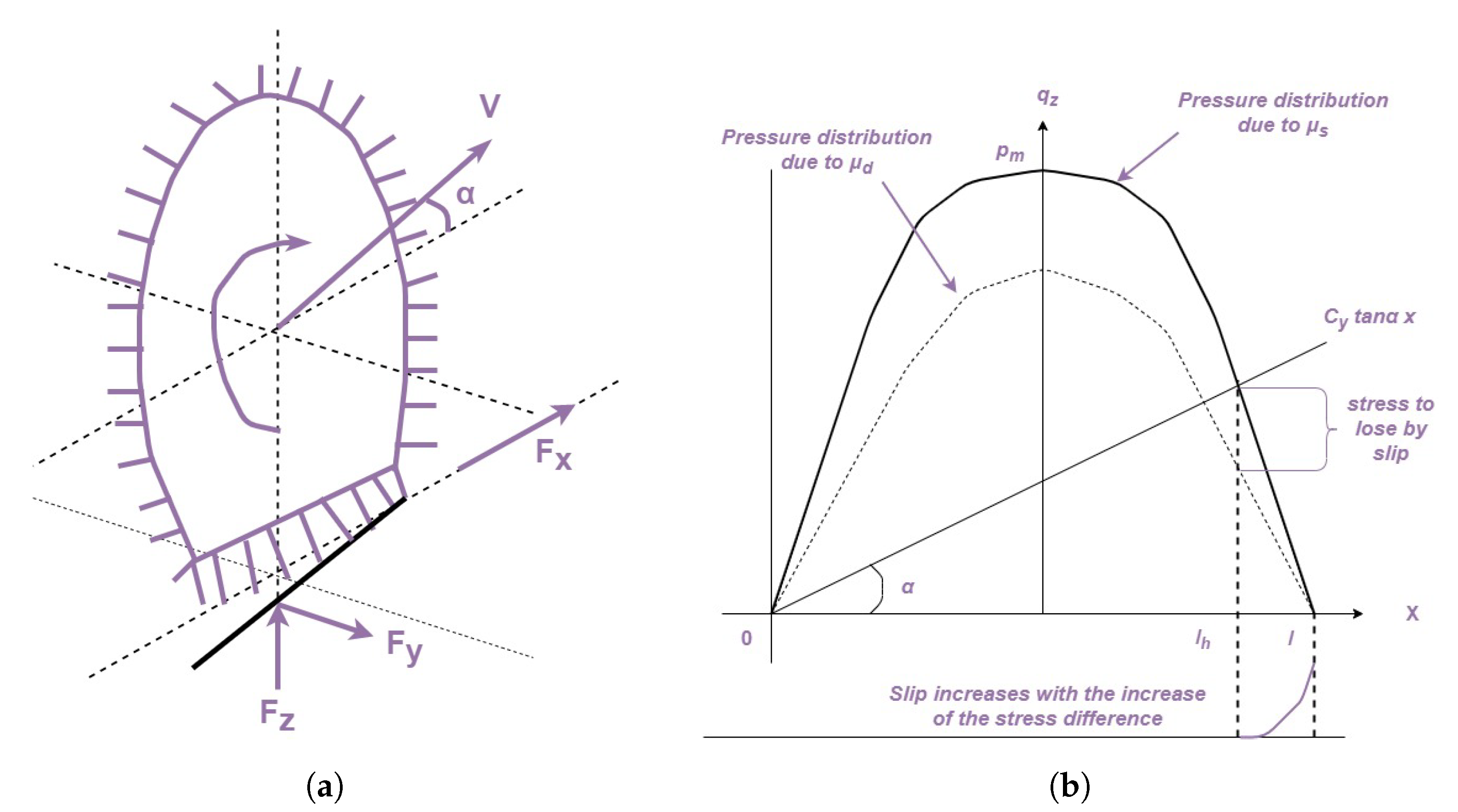
Semi-active suspensions do not consume significant amount of energy and can provide a more energy efficient solution compared to fully active ones. At the same time, the reliability of passive suspensions can be maintained. Therefore, different control strategies have been developed exploiting the benefits of semi-active suspensions. In this work, the suspension system of the vehicle model operates as passive (PS) and semi-active. Several different control algorithms are used in the semi-active suspension case: SH-2 [30], ADD [31], SH-ADD-2 [32], PDD [33], SH-PDD [34] and GH-2 [35]. The operational conditions of the semi-active control algorithms are illustrated in

Table 2. Semi-active control algorithms applied in the vehicle suspension systems (Figure 2).

Case	Description	Control Law a
1	SH-2	$C_u=\left\{\begin{array}{cc}{C}_{min}\hfill & ,if {\dot{d}}_{ST}{\dot{z}}_s<0\hfill \\ C_{max}\hfill & ,if {\dot{d}}_{ST}{\dot{z}}_s>0\hfill \end{array}\right.$
3	ADD	$C_u=\left\{\begin{array}{cc}{C}_{min}\hfill & ,if {\dot{d}}_{ST}{\ddot{z}}_s\le 0\hfill \\ C_{max}\hfill & ,if {\dot{d}}_{ST}{\ddot{z}}_s>0\hfill \end{array}\right.$
4	SH-ADD-2 b	$C_u=\left\{\begin{array}{cc}{C}_{min}\hfill & ,if {\ddot{z}}_s^2-a_f^2{\dot{z}}_s^2\ge 0\hfill \\ C_{max}\hfill & ,if {\ddot{z}}_s^2-a_f^2{\dot{z}}_s^2<0\hfill \end{array}\right.$
5	GH-2	$C_u=\left\{\begin{array}{cc}{C}_{min}\hfill & ,if {\dot{d}}_{ST}{\dot{z}}_u>0\hfill \\ C_{max}\hfill & ,if {\dot{d}}_{ST}{\dot{z}}_u<0\hfill \end{array}\right.$
6	PDD	$C_u=\left\{\begin{array}{cc}{C}_{min}\hfill & ,if K_u{\dot{d}}_{ST}+C_{min}{\dot{d}}_{ST}^2\ge 0\hfill \\ C_{max}\hfill & ,if K_u{\dot{d}}_{ST}+C_{min}{\dot{d}}_{ST}^2<0\hfill \\ \\ \frac{C_{min}+C_{max}}{2}\hfill & ,if d_{ST}\ne 0\mathrm{and}{\dot{d}}_{ST}=0\hfill \\ \\ \frac{-K_u{d}_{ST}}{{\dot{d}}_{ST}}\hfill & ,otherwise\hfill \end{array}\right.$
7	SH-PDD	$C_u=\left\{\begin{array}{cc}{C}_{SH-2}\hfill & ,if {\dot{z}}_s^2-{\dot{z}}_s^2\ge 0\hfill \\ C_{PDD}\hfill & ,otherwise\hfill \end{array}\right.$

^a The parameter $d_{ST}$ refers to the vehicle suspension travel, i.e., $z_s-z_u$, while ${\dot{d}}_{ST}$ is the vehicle suspension velocity, i.e., ${\dot{z}}_s-{\dot{z}}_u$. ^b The parameter ${\alpha }_f$ is the crossover frequency between SH-2 and ADD ∈ [10–60] $\frac{rad}{sec}$.

.

2.3. Tread Model

In order to evaluate the wear quantity, the energy loss has to be calculated, hence the contact between the tyre and the road should be modelled with regards to that and not only with spring and dampers as usual. Therefore, this model considers that the tread. which is in contact with the road surface ($z_R$), is a cuboid element with a, b and h being its length, width and height, respectively (Figure 3a). Regarding the first two, they are evaluated according to empirical equations (Equation (4)) [9,36], which consider tyre dimensions, i.e., the outside radius (d) and the crown thickness ($b_0$), and its deformation ($\delta$):

$$a=4d{\left(\frac{\delta }{2d}\right)}^s,b=b_0(1-e^{-\psi })$$

(4)

where $\psi$ (=115) and s (=0.67) are empirical coefficients. The tyre deformation ($\delta$) is evaluated according to Equation (5):

$$\delta =\frac{{\alpha }_1{F}_z}{2P}+\sqrt{{\left(\frac{{\alpha }_1{F}_z}{2P}\right)}^2+{\alpha }_2{F}_z}$$

(5)

where ${\alpha }_1$ is $1/\left(2\pi d{r}_w\right)$, with $r_w$ being the tyre chordwise curvature radius; ${\alpha }_2$ (=$3.70\ast {10}^{-8}$) is a constant for car tyre; and $F_z$ is the wheel load. According to $\delta$ (Equation (5)), the tread deformation is related with the pressure (P) (Figure 3b), the tyre radius (d) and the chordwise radius ($r_w$). The force–deflection curves that occur through Equation (5) are plotted in Figure 3b for different tyre pressures (P). Finally, the mass of the tread element can be derived by Equation (6), where $\rho$ (=1156 kg/m${}^3$) is the rubber density of the tread.

$$m_t=abh\rho$$

(6)

2.4. Vehicle Performance Assessment

2.4.1. Tyre Wear Quantity

Tyre wear is defined according to the frictional or wear energy, $E_w$[Nm/m${}^2$], which is the energy due to slippage per unit area and can be evaluated as the product of the shear stress ($\overrightarrow{\tau }$) and slip ($\overrightarrow{S}$):

$$E_w={\int }_0^b\overrightarrow{\tau }d\overrightarrow{S}$$

(7)

where b is the contact length; ${\tau }_x$ and ${\tau }_y$ are, respectively, shear stresses in x- and y-directions; and $S_x$ and $S_y$ are, respectively, slip distances in x- and y-directions.

Wear energy during cornering: In order to calculate the wear energy ($E_w$) during cornering, a solid tyre is considered using a brush model (Figure 4a), while, for the wear evaluation during cornering, a wear model is used (Figure 4b). In the considered wear model, parabolic pressure distribution ($q_z$) and small slip angles are assumed. The contact pressure is defined as:

$$q_z=4p_m\frac{x}{b}\left(1-\frac{x}{b}\right)$$

(8)

where $p_m$ is the maximum pressure that occurs from the vertical load $F_z$ and is equal to $3F_z/2ab$ if the contact patch is assumed as cuboid (Figure 3a). According to the wear model (Figure 4b), the lateral slip angle is $\alpha$, while the lateral shear stress at a distance x measured from the the contact patch (0–b) is ${\tau }_y$ and is expressed by Equation (9):

$${\tau }_y=C_{y}xtan\alpha$$

(9)

where $C_y$ [N/m] is the lateral shear elastic tread coefficient per unit area. The shear force ${\tau }_z$ (=${\mu }_s{q}_z{b}_h$) applied to the contact patch per unit area is equal to the lateral shear stress applied to the sliding point $b_h$ (Equation (9)), i.e., the maximum frictional force per unit area (${\tau }_{y_{max}}$). Therefore, combining Equations (8) and (9):

$${\tau }_{y_{max}}=C_y{b}_{h}tan\alpha ={\mu }_s{q}_z\left(b_h\right)=4{\mu }_s{p}_m\frac{x}{b_h}\left(1-\frac{x}{b_h}\right)$$

(10)

where ${\mu }_s$ is the static friction coefficient, while $\zeta$$\left(=\frac{C_{y}btan\alpha }{4{\mu }_s{p}_m}\right)$ is introduced as a new coefficient, to help in the simplification of the equations. Based on $\zeta$, the sliding point ($b_h$) is defined as:

$$\begin{array}{ccc}\hfill b_h=& b(1-{\zeta }_h)\hfill & \hfill ,0\le {\zeta }_h\le 1\\ \hfill b_h=& 0\hfill & \hfill ,1>{\zeta }_h\end{array}$$

(11)

where the first part is when the tyre is in the adhesion region, while the second part considers that sliding occurs across the whole contact area when ${\zeta }_h$ is greater than or equal to unity. Then, considering the force equilibrium in the sliding region ($b_h\le x\le b$), the sliding distance is defined according to Equation (12), where ${\mu }_d$ is the kinematic friction coefficient:

$$S_y=xtan\alpha -\frac{{\mu }_d{q}_z\left(x\right)}{C_y}$$

(12)

Considering Equation (7), the wear energy per unit area is defined as:

$${E_y}^w={\int }_{b_h}^b{\mu }_d{q}_z\left(x\right)d{S}_y={\int }_{b_h}^b{\mu }_d{q}_z\left(x\right)\frac{d{S}_y}{dx}dx={\mu }_{d}tan\alpha {\int }_{b_h}^b{q}_z\left(x\right)dx+\frac{1}{2}\frac{{\mu }_d^2}{C_y}{q}_z^2\left(b_h\right)$$

(13)

where Equations (8) and (11) can be substituted, and the equation of wear energy can be derived at the two conditions explained in Equation (11). In addition, in this work, ${\mu }_d$ and ${\mu }_s$ are assumed to be equal to $\mu$, while $F_z$ is considered from the vehicle model:

$$F_z=F_{Z_0}+C_t({\dot{z}}_t-{\dot{z}}_R)+K_t(z_t-z_R)$$

(14)

where $F_{Z_0}$ is the static load applied.

Mass Loss: The wear energy per contact area described above can be related with the mass loss according to Equation (15), which was derived by Lupker et al. [17] from experiments:

$$\Delta m=f_1{E}^{f_2}$$

(15)

where $f_1$ and $f_2$ are constants at a given temperature. The mass loss ($\Delta m$) evaluated at each time step is used to calculate the $m_t$ dynamically. As an extension of this expression, Li et al. [14] redefined $f_1$ by incorporating in it the effect of temperature:

$$\Delta m=f_{0}1.{02}^{T_t-T_0}{E}^{f_2}$$

(16)

where $f_2$ is $1.5106$ and $f_0$ (=$2.{010}^{-10}$) is the constant $f_1$ at $T_0$ (=${60}^{\circ }$). $T_t$ is defined as the steady state temperature of the tyre tread:

$$T_t=\frac{0.0447\gamma {(3.6\ast V)}^{0.16}{F}_z{d}^{-0.5}{\delta }^{0.5}}{\pi \beta [2dc+0.4(d^2-r^2)+0.4(d^2+dr+r^2)-0.6r(d+r)]}+T_{\infty }$$

(17)

where V[m/s] is the vehicle velocity; r is rim radius; c is the tyre width; $\gamma$ (=$0.12$) is the tyre hysteresis coefficient; $\beta$ (=$1.40$) is the correction coefficient; and $T_{\infty }$ is the ambient temperature.

Wear quantity: The total wear quantity that is caused by the mass loss (Equation (16)) is defined as the height change ($\Delta h$):

$$\Delta h=\frac{\Delta m}{\rho ab}$$

(18)

Finally, the total tread wear is defined:

$$\begin{array}{ccc}\hfill H\left(t\right)=& \Delta h\hfill & \hfill ,t\le t_0\\ \hfill H\left(t\right)=& H(t-t_0)+\Delta h\hfill & \hfill ,t>t_0\end{array}$$

(19)

where $H(t-t_0)$ is the total tread wear occurred during the first tyre revolution taking place as long as $t\le t_0$, with $t_0$ (=$2\pi r_r/V$) being the rotating period and $r_r$ the rolling radius.

2.4.2. Ride Comfort

Ride comfort (RC) is assessed via the root mean square of the sprung mass’ vertical acceleration (${\ddot{z}}_s$), when measurements are not applicable to the seat or the occupant’s body [37]. More specifically, $RC$ is calculated as follows:

$$RC={\left[\frac{1}{T}\left({\int }_0^T{\ddot{z}}_{w_z}{\left(t\right)}^{2}dt\right)\right]}^{\frac{1}{2}}=RMS\left({\ddot{z}}_{w_z}\right)$$

(20)

where T ($\left[s\right]$) is the duration and ${\ddot{z}}_{w_z}$ (m/s${}^2$) is the weighted acceleration as a function of time. In this work, no weighting is applied in the accelerations measured at the sprung mass. Therefore, ${\ddot{z}}_{w_z}$ is considered equal to ${\ddot{z}}_s$.

2.4.3. Vehicle Handling

The vehicle handling is normally assessed through cornering, braking and traction abilities, which all are enhanced if the tyre loads/deflections are maintained at a low level. Therefore, the root mean square of the tyre deflection ($z_u-z_{Road}$) is considered as an index (Equation (21)) for vehicle stability (Figure 2), taking advantage of the available outputs from the vehicle model:

$$TD={\left[\frac{1}{T}\left({\int }_0^T{(z_u-z_{Road})}^{2}dt\right)\right]}^{\frac{1}{2}}$$

(21)

At the same time, the suspension travel depicts the ability of the suspension system to support and hold the vehicle load. This is achieved when rattle space requirements of the vehicle are kept small. Therefore, the root mean square of the suspension travel ($z_s-z_u$) is considered as an index (Equation (22)) for vehicle stability as well:

$$ST={\left[\frac{1}{T}\left({\int }_0^T{(z_s-z_u)}^{2}dt\right)\right]}^{\frac{1}{2}}$$

(22)

2.5. Road Profiles and Path

The combination of the vehicle model with the above analysis on the wear quantity allows the assessment of the wear under different conditions (i.e., road surfaces, paths and vehicle velocities), tyres and vehicle types. More specifically, different road surfaces can be used for exciting the vehicle model and different paths can be considered by applying in the wear model the vehicle’s corresponding slip angles and velocities while driving on any path. The vehicle’s corresponding slip angles and velocities have to be obtained from offline simulations prior to the simulation of the vehicle model.

In this work, road profiles of Class A and B (Figure 5a) are used to excite the vehicle model and are designed according to ISO-8608 [38]. Then, the S-path illustrated in Figure 5b, which consists of two turns of different radius (70 and 60 m), is used to extract the slip angles and the vehicle velocity while driving on it. In this work, both are obtained from simulating the demo vehicle of IPG/CarMaker 8.0, IPG AUTOMOTIVE, Braunschweig, Germany (Figure 6) while driving over the S-path, having assigned on it the two road profiles.

3. Validation of the Model with IPG CarMaker 8.0

In order to secure that the optimisation results in this work are realistic, the model is validated using IPG/CarMaker 8.0 for the path illustrated in Figure 5b and the road profile of Class B assigned to it (Figure 5a).

As mentioned above, the vehicle parameters selected for the model are extracted from the software demo vehicle to build its digital twin. The suspension and tyre parameters of the models are adjusted according to Table 1 and

Table 3. Wear and tread model parameters.

Wear and Tread Model Parameters
$\mathit{P}$[KPa]	$\mathit{c}$[m]	$\mathit{d}$[m]	${\mathit{b}}_{\mathbf{0}}$[m]	${\mathit{r}}_{\mathit{w}}$[m]
250	0.1950	0.3175	0.1660	0.1550

. More specifically, the suspension parameters (Table 1) of the front wheels are adjusted into the section Car/VehicleDataSet/Suspensions of the software. Regarding the suspensions, for both the stiffness and the damping coefficient, a characteristic value option is selected, while the values of the buffer are set zero in the software, as the buffer is not included in the model. Then, regarding the tyres, the parameters related with them and considered in the vehicle and wear model (P, d, c, r, $K_T$ and $C_T$), are adjusted according to section Tires/TireDataSet/GeneralandModelParameters of the software. The only parameters that are not provided are the crown thickness ($b_0$), the chordwise curvature ($r_w$) and the lateral shear elastic tread coefficient ($C_y$). Regarding the first two, its consideration is not possible, but $C_y$ is extracted after evaluating it using the cornering stiffness obtained from the software simulation results. More specifically, the side force applied in the wheel for a rectangular contact area, as in this case, can be evaluated for small slip angles:

$$F_y={\int }_0^b{f}_{y}dx=C_{y}a{\int }_0^{b}Vdx=C_{y}a{\int }_0^{b}x\alpha dx=\frac{C_{y}a{b}^2}{2}\alpha$$

(23)

Thus, according to Equation (23), the cornering stiffness $C_{Fa}$ is equal to $\frac{C_{y}a{b}^2}{2}\alpha$. Therefore, after fitting the simulation results (lateral slip angles and side forces) to a linear equation, as shown in Figure 6b, the value of $C_y$ is extracted.

Having created the digital twin of the demo vehicle (Figure 6), the wear energy ($E_y$[Nm/m${}^2$]) is selected for comparison in order to validate the simulation results. Therefore, the obtained measurements are used as follows for calculating the wear energy ($E_{y_{carmaker}}^w$):

• The sliding distance ($s_d$) is calculated according to Equation (12).
• The parameter ($\varphi$) is calculated as follows:

  $$\varphi =\frac{C_{Fa}\left|tan\alpha \right|}{\mu F_z}.$$

  (24)
• The sliding force is obtained by integrating the maximum possible frictional force distribution ($\mu q_z$) over the sliding region $b_h\le x<b$:

  $$F_{slid}={\int }_b^{b_h}\mu q_{z}dx=\mu F_z\left(\frac{1}{3}{\varphi }^2-\frac{2}{27}{\varphi }^3\right)sign\left(a\right).$$

  (25)
• Finally, the wear energy per contact area according to Equation (26) is evaluated by multiplying the sliding force with the slipping distance ($S_y$) and dividing it by the contact area:

  $$E_{y_{carmaker}}^w=\frac{F_{slid}{S}_y}{a\ast b}.$$

  (26)

The comparison of $E_{y_{carmaker}}^w$ with $E_y^w$ is illustrated in Figure 7, which proves a good convergence in the two simulation results. More specifically, Figure 7 illustrates high similarity in terms of the trend of the two curves. Slight differences occur in the magnitude with the model used in this work underestimating a few of the peaks. However, this underestimation is not an issue as the trend is accurately followed, and, given the simplicity of the model in comparison with IPG/CarMaker 8.0, the results should be considered valid.

4. Optimisation Configuration

In this work, the emphasis is on the optimisation of tyre and suspension parameters for minimising tyre wear. However, as comfort and vehicle stability are still important criteria in the design process, they are also included as objectives by configuring a multi-objective optimisation problem. In order to decrease the complexity of the optimisation, the tyre and suspension parameters are optimised separately considering two optimisation scenarios. Initially, the optimal tyre design solutions (Scenario 1) are sought for the vehicle equipped with a passive suspension, while driving over a road class A (Case 1) and B (Case 2) S-path (Figure 5). Then, after selecting one of the optimal tyre design solutions, which can provide similar tyre wear for both road profiles, the optimal suspension designs (Scenario 2) are sought for different suspension types, both passive and semi-active (PS, SH-2, ADD, SH-ADD-2, PDD, SH-PDD and GH-2), for the two road cases.

4.1. Objectives

The multi-objective optimisation problem is formulated in order to minimise tyre wear, enhance ride comfort and increase vehicle handling at the same time. In both scenarios, wear and comfort are represented from the same objective function ($F_1$ and $F_2$), whereas vehicle handling ($F_3$) is represented with the most suitable function according to the scenario. In Scenario 1, where the tyre is optimised, $TD$, defined in Equation (21), is selected as the objective function, while, in Scenario 2, where the focus is on the suspension, $ST$ is selected, as defined in Equation (22).

$$\mathrm{Scenario}1:F_1=max\left(H\left(t\right)\right);F_2=R{C}_z;F_3=TD;$$

(27)

$$\mathrm{Scenario}2:F_2=max\left(H\left(t\right)\right);F_2=R{C}_z;F_3=ST;$$

(28)

In both scenarios, the optimisation is conducted using the GAMULTIOBJ toolbox from MATLAB 2017b, where the $PopoulationSize$ is selected as 250 and the $EliteCount$ as 5. The rest of the options are selected according to the default suggestions from the software.

4.2. Design Variables: Scenario 1

In this scenario, the following design variables are selected:

$$P,c,d,b_0\mathrm{and}{r}_w$$

(29)

while the upper and lower bounds set are illustrated in

Table 4. Design variables and their bounds for Cases 1 and 2.

Scenario 1			Scenario 2
Design Variable	Bounds		Design Variable	Bounds
	$\mathit{LB}$	$\mathit{UB}$		$\mathit{LB}$	$\mathit{UB}$
P[KPa]	150	350	$K_u$ [N/m]	15,000	60,000
c[m]	0.14	0.22	$C_u$ [Ns/m]	500	5000
d[m]	0.27	0.35	$C_{min}$[Ns/m]	500	2500
$b_0$[m]	0.12	0.19	$C_{max}$ [Ns/m]	2500	5000
$r_w$ [m]	0.12	0.20	${\mathrm{a}}_f$ [rad/s] a	10	60

^a The parameter ${\alpha }_f$ is included as a design variable for Case 2 only when the SH-ADD2 is optimised.

. In addition, $K_t$ and $K_T$ might be considered indirect design variables as they are evaluated according to the problem design variables. More specifically, during the optimisation, the force–deflection curve (Figure 3b) is evaluated according to Equation (5), which is a relation of P, d and $r_w$, for $F_z$ varying from 500 to 7000 N for each potential optimal solution. Then, having obtained the force–deflection curve, the $K_t$ is evaluated as the curve slope at the linear region, while the sidewall stiffness ($K_T$) is evaluated by $0.8\ast K_t$ as the sidewall is always less stiff than the tread.

4.3. Design Variables: Scenario 2

Regarding the second scenario, where the optimum designs are sought for the different suspension types, the design variables shown in Equations (30)–(32) are selected:

For PS:

$$K_u,C_u$$

(30)

For SH-2, ADD, GH-2, PDD and SH-PDD:

$$K_u,C_{min}\mathrm{and}{C}_{max}$$

(31)

For SH-ADD2:

$$K_u,C_{min},C_{max}\mathrm{and}{a}_f$$

(32)

while the upper and lower bounds set in the optimisation are illustrated in Table 4.

5. Results

As described above, in this work, two optimisation cases, with regards to different excitations, are studied in two optimisation scenarios where the focus is on tyre and suspension design, respectively. In this section, the results of the two multi-objective optimisation scenarios are displayed. More specifically:

• Scenario 1 investigates the tyre optimisation in a vehicle being employed with a passive suspension and driven over an S-Path, in which road surfaces of Class A (Case 1) and B (Case 2) are assigned. The optimisation results are illustrated in Figure 8 and Figure 9, which display the Pareto fronts with regards to the objectives (Figure 8a,b) and the design variables (Figure 9a–e). Having obtained the optimal solution alternatives for the two cases, common solutions are sought between them, requiring to provide similar wear in the two cases (<8% difference) and have close design variable values (<9% difference). The common solutions identified with the above characteristics are illustrated in Figure 8 and Figure 9 alongside the alternatives, while their values are listed in

  Table 5. Optimal tyre design variables of the identified common solutions among the two cases of different road profiles.

  Solution	Optimum Design Variables
  	P[KPa]	c[m]	d[m]	${\mathit{b}}_0$[m]	${\mathit{r}}_{\mathit{w}}$[m]
  1	252	0.1889	0.2728	0.1215	0.1420
  2	192	0.1883	0.2746	0.1206	0.1441

  . In addition, in Figure 10, the final circumferential tread profiles for the optimum designs are compared with the initial tyre design, after driving over the Class B S-Path twenty times back and forth.
• Scenario 2 explores the suspension optimisation for two road cases and various suspension types (PS, SH-2, ADD, SH-ADD-2, GH-2, PDD and SH-PDD). The optimisation results are illustrated in Figure 11, which presents the Pareto fronts of the optimum solutions for the two cases. For each suspension type, a common solution is identified among the optimal alternatives provided by the two optimisation cases, requiring them to have close design variables values (<3–15% difference according to the cases). Finally, the values of the identified common solutions are presented in

  Table 6. Common optimal suspension parameters among the two road profile cases for each suspension type.

  Solution	Optimum Design Variables
  	${\mathit{K}}_3$[N/m]	${\mathit{C}}_{\mathbf{min}}$[Nm/s]	${\mathit{C}}_{\mathbf{max}}$[Nm/s]	${\mathit{a}}_{\mathit{f}}$ [rad/sec]	Threshold ($\mathit{\epsilon }$)
  PS	16,042	3675	-	-	6.0%
  SH-2	43,181	2275	4394	-	9.5%
  GH-2	16,160	2415	3327	-	3.0%
  ADD	41,406	2452	4530	-	5.0%
  PDD	15,534	1442	4045	-	5.0%
  SH-PDD	42,281	2416	4749	-	5.0%
  SH-ADD2	17,246	684	3515	23.5	15.0%

  alongside with the threshold of difference that was allowed.

The goal of these scenarios is for conclusions to be extracted regarding: $\left(a\right)$ how tyre wear behaves with regards to passenger comfort and vehicle handling; $\left(b\right)$ where optimum tyre and suspension parameters have converged trying to compromise among the above objectives under different road types; and $\left(c\right)$ which suspension could compromise among all of them optimally.

5.1. Optimum Tyre Design Solutions

Optimisation Results

Regarding Scenario 1, Figure 8a,b illustrates the relation between the optimisation objectives and reveals the trade-offs among them. More specifically, Figure 8a reveals the conflicting relation between wear and comfort levels, where the increase of the RC index, which yields the increase of discomfort, leads to the decrease of tyre wear. At the same time, the conflicting relation of comfort and handling, captured by the optimisation in Figure 8b, serves as an indication of the validity of the results. In addition, the conflicting relation of the two objectives, handling and wear, with comfort reveal the linear relation between them, implying that increased levels of tyre deflections lead to increasing wear.

As far as the design variables are concerned, according to Figure 9a–e, the tyre pressure (P), the outside radius (d) and the chordwise curve ($r_w$) illustrate a conflicting relation with wear. For these, the algorithm has provided optimal alternatives ranging from the lower bound to the upper bound, which allowed capturing the conflicting relation between these variables and wear. On the other hand, the Pareto alternatives of tyre width (c) and crown thickness ($b_0$), as shown in Figure 9b,d, respectively, have not captured their relation with wear, as the algorithm converged close to one value. In the case of the tyre width, this value is different from the upper or lower bound, whereas the crown thickness alternatives have converged close to the lower bound trying to decrease the length of the tread (Figure 3a). However, both values are realistic according to the literature.

Regarding the different road cases, Case 2 alternatives are providing larger values in all the objectives, as the more intense road roughness profile has increased discomfort, vehicle instability and tyre wear. Regarding the latter, according to Figure 8a, Case 2 Pareto alternatives have increased wear around ∼25% compared to Case 1, which illustrates how road profiles increase wear significantly if different tyre designs are adopted. In terms of convergence, Case 2 has provided more scattered fronts in both the objective and the design variables fronts, illustrating that the less intense excitation (Case 1 with Class A road roughness) allowed the algorithm to converge to a more solid Pareto front. However, in both cases, the alternatives mostly have captured the same conflicting relations, while the design variables are within the same range of values.

Finally, as mentioned above, common solutions are sought requiring for them to provide similar wear in the two cases (<8% difference) and have close design variables values (<9% difference). This search led to two common solutions between the optimal alternatives of the two cases, as pointed out in Figure 8 and Figure 9 and Table 5. Based on these, in Case 1 where road Class A is considered, the common solutions are closer to the upper edge of the Pareto front, being more comfort oriented in this case, while in Case 2 they are closer to the lower edge, being more stability oriented. Regarding their design variable values (Table 4), they are all the same with only the pressure ($P_t$) being significantly different. This outcome of the optimisation implies that the optimum tyre design has two pressures (P) with which it can drive optimally over both a road Class A and B S-path with the same levels of wear. The similarity of these two solutions in terms of the overall wear is illustrated in Figure 10, where the circumferential tread profile that occurs with these solutions is compared along with the one that would occur with the initial tyre design, as shown in Table 3. In addition, Figure 10 displays how the optimisation has improved the tread circumferential profile by not only minimising the overall wear, but also smoothening the variations compared to the initial solution.

5.2. Optimum Suspension Design

Regarding Scenario 2 and the suspension optimisation, the Pareto fronts of the different suspension types with regards to the three optimisation objectives are illustrated in Figure 11, while the common solutions identified are pointed out in Figure 11a.

Based on the results in Figure 11b,e, the relation between comfort and handling is consistent with what was expected, illustrating the conflict between the two objectives. At the same time, the optimisation algorithm has converged to solutions with similar wear characteristics for most of the suspension types as the wear objective has small differences (Figure 11a,c,d), especially for Case 1. On the one hand, the above outcomes imply that for a suspension system, after having decided the appropriate suspension type and the optimal tyre design with regards to wear, the engineers can focus on the rest of the objectives to tune the suspension optimally. On the other hand, different control algorithms could make a significant difference in terms of the tyre wear performance. According to the Pareto fronts, the increase of the wear from Case 1 (Figure 11a, Class A) to Case 2 (Figure 11d, Class B) is ∼13% for most of the semi-active suspensions, illustrating their lack of adaptability in different road profiles. However, SH-2 and SH-ADD-2 (Figure 11c) provide the minimum levels of wear, with insignificant differences between them, and maintained the same tyre wear levels for the two cases.

Regarding the compromise between comfort and vehicle handling, the Pareto fronts of all the suspension types in both cases have similar trends, and they validate the theoretical basis of each control algorithm. More specifically, SH-ADD2 is trying to balance the characteristics of SH-2 and ADD, with its Pareto alternatives being between the SH-2 and ADD Pareto fronts. In this direction, the SH-ADD2 Pareto front connects the upper part of the SH-2 front (the stability oriented) and the lower part of the ADD front (the comfort oriented). Similarly, SH-PDD is trying to balance the characteristics of SH-2 and PDD with its Pareto front alternatives being between those of SH-2 and PDD, while it also connects the upper part of the PDD front (the comfort oriented) and the lower part of the SH-2 front (the stability oriented). At the same time, GH-2 is providing solutions with more vehicle stability but less comfort. Finally, the PS Pareto alternatives in both cases include solutions that could replace few semi-active algorithms (SH-ADD2, PDD and ADD) but with slightly either less comfort or less vehicle handling.

As far as the common solutions are concerned, in most of the suspension types, the common identified solution between the two road cases is one that enhances comfort more, being in the top part of the Pareto font (Figure 11a). Only in PDD, the common solution is located at the bottom part of the Pareto front, as shown in Figure 11a, which is the one that emphasises vehicle handling. The design variables are are illustrated in Table 6. Based on Table 6, for a few of the suspension types (PS, GH-2, PDD and SH-ADD2), the design variables have converged to a soft spring, while the rest (SH-2, ADD and SH-PDD) to a much stiffer one. Regarding, SH-2 and SH-ADD-2, which are the ones that provide similar tyre wear levels for both road profiles, they have converged to different suspension tuning and also the common solution was identified with a high allowed threshold, which could be the reason these two algorithms provide minimum tyre wear for the two road cases. The first has converged to a stiff spring and damper coefficient for both $C_{min}$ and $C_{max}$, however the comfort levels are maintained to good levels for both road cases. On the other hand, SH-ADD-2 has converged to a soft suspension design, with spring ($K_3$) and damping coefficients ($C_{min}$) close to the lower bounds allowed by the optimisation. However, the vehicle handling is maintained to similar levels with the SH-2 solution.

6. Conclusions

To sum up, this work considers a vehicle model combined with a tyre wear model in order to optimise tyre and suspension parameters to minimise tyre wear, enhance comfort and improve stability. In addition to the search for the optimum tyre and suspension design, the optimisation is also used as the tool to identify any conflicting or not relations between the design variables and the optimisation objectives.

In summary, the following conclusions are extracted.

• Comfort illustrates the same conflicting relation with wear as with vehicle stability. This means that the increase of the suspension travel, hence degradation of handling, leads to an increase in wear but to an improvement in comfort.
• Wear could increase up to 21% in different road profiles, while the appropriate tyre design could provide only 2% increase if the road roughness changes from Class A to B. The appropriate tyre design could be extracted using the optimisation method proposed in the current work.
• For the same tyre design, two pressures could optimally combine comfort, wear and stability in two road roughness cases but also maintain wear at the same levels in these two cases. The recursive feasibility of this outcome should be tested, but it is an interesting remark for the current case study.
• Regarding suspension types, according to the results, the type and their control algorithm should be selected with regards to tyre wear damage. In the current case study, SH-2 and SH-ADD-2 seemed to be able to provide the best wear performance. After the selection of the control algorithm, the tuning of the suspension parameters, i.e., stiffness and damping coefficient, should take place mainly with regards to comfort and vehicle handling. This is because according to the results it seems that different configurations do not affect wear to a great extent.

Further work is in progress to develop active suspension systems using novel control algorithms to decrease wear. At the same time, tyre and suspension design should be investigated in depth with regards to the tyre wear using more detailed wear and vehicle models. Finally, their experimental validation and investigation is an aspect that should be considered further.

References

1. Sambito, M.; Severino, A.; Freni, G.; Neduzha, L. A systematic review of the hydrological, environmental and durability performance of permeable pavement systems. Sustainability 2021, 13, 4509. [Google Scholar] [CrossRef]
2. Jan Kole, P.; Löhr, A.J.; Van Belleghem, F.G.; Ragas, A.M. Wear and tear of tyres: A stealthy source of microplastics in the environment. Int. J. Environ. Res. Public Health 2017, 14, 1265. [Google Scholar] [CrossRef]
3. Grigoratos, T.; Gustafsson, M.; Eriksson, O.; Martini, G. Experimental investigation of tread wear and particle emission from tyres with different treadwear marking. Atmos. Environ. 2018, 182, 200–212. [Google Scholar] [CrossRef]
4. Wik, A.; Dave, G. Occurrence and effects of tire wear particles in the environment—A critical review and an initial risk assessment. Environ. Pollut. 2009, 157, 1–11. [Google Scholar] [CrossRef]
5. Webster, B. Tyres of electric cars add to air pollution, experts warn. The Times. 7 December 2020. Available online: https://www.thetimes.co.uk/article/electric-car-tyres-are-growing-source-of-air-pollution-28276fmdp#:~:text=Electric%20cars%20with%20heavy%20batteries,road%20surface%2C%20experts%20have%20recommended (accessed on 25 June 2021).
6. Fuller, G. Pollutionwatch: How smart braking could help cut electric car emissions. The Guardian. 29 January 2021. Available online: https://www.theguardian.com/environment/2021/jan/29/pollutionwatch-how-smart-braking-could-help-cut-electric-car-emissions (accessed on 25 June 2021).
7. Knisley, S. A correlation between rolling tire contact friction energy and indoor tread wear. Tire Sci. Technol. TSTCA 2002, 30, 83–99. [Google Scholar] [CrossRef]
8. Huang, H.; Chiu, Y.; Wang, C.; Jin, X. Three-dimensional global pattern prediction for tyre tread wear. Proc. Inst. Mech. Eng. Part D J. Automob. Eng. 2015, 229, 197–213. [Google Scholar] [CrossRef]
9. Nakajima, Y. Advanced Tire Mechanics; Springer: Singapore, 2019; pp. 1–1265. [Google Scholar] [CrossRef]
10. Maître, O.L.; Süssner, M.; Zarak, C. Evaluation of Tire Wear Performance; SAE Technical Papers; SAE International: Warrendale, PA, USA, 1998. [Google Scholar] [CrossRef]
11. Ma, B.; Xu, H.g.; Chen, Y.; Lin, M.y. Evaluating the tire wear quantity and differences based on vehicle and road coupling method. Adv. Mech. Eng. 2017, 9, 168781401770006. [Google Scholar] [CrossRef] [Green Version]
12. da Silva, M.M.; Cunha, R.H.; Neto, A.C. A simplified model for evaluating tire wear during conceptual design. Int. J. Automot. Technol. 2012, 13, 915–922. [Google Scholar] [CrossRef]
13. Sueoka, A.; Ryu, T.; Kondou, T.; Togashi, M.; Fujimoto, T. Polygonal Wear of Automobile Tire. JSME Int. J. Ser. C 1997, 40, 209–217. [Google Scholar] [CrossRef] [Green Version]
14. Li, Y.; Zuo, S.; Lei, L.; Yang, X.; Wu, X. Analysis of impact factors of tire wear. J. Vib. Control 2011, 18, 833–840. [Google Scholar] [CrossRef]
15. Stalnaker, D.; Turner, J.; Parekh, D.; Whittle, B.; Norton, R. Indoor Simulation of Tire Wear: Some Case Studies. Tire Sci. Technol. TSTCA 1996, 24, 94–118. [Google Scholar] [CrossRef]
16. Knuth, E.F.; Stalnaker, D.O.; Turner, J.L. Advances in Indoor Tire Tread Wear Simulation; SAE Technical Papers; SAE International: Warrendale, PA, USA, 2006. [Google Scholar] [CrossRef]
17. Lupker, H.; Cheli, F.; Braghin, F.; Gelosa, E.; Keckman, A. Numerical prediction of car tire wear. Tire Sci. Technol. TSTCA 2004, 32, 164–186. [Google Scholar] [CrossRef]
18. Braghin, F.; Cheli, F.; Melzi, S.; Resta, F. Tyre wear model: Validation and sensitivity analysis. Meccanica 2006, 41, 143–156. [Google Scholar] [CrossRef]
19. Farroni, F.; Sakhnevych, A.; Timpone, F. Physical modelling of tire wear for the analysis of the influence of thermal and frictional effects on vehicle performance. Proc. Inst. Mech. Eng. Part J. Mater. Des. Appl. 2017, 231, 151–161. [Google Scholar] [CrossRef]
20. Emami, A.; Khaleghian, S.; Bezek, T.; Taheri, S. Design and development of a new portable test setup to study friction and wear. Proc. Inst. Mech. Eng. Part J J. Eng. Tribol. 2020, 234, 730–742. [Google Scholar] [CrossRef]
21. Lepine, J.; Na, X.; Cebon, D. An Empirical Tire-Wear Model for Heavy-Goods Vehicles. Tire Sci. Technol. 2021, 49. [Google Scholar] [CrossRef]
22. Yamazaki, S.; Fujikawa, T.; Hasegawa, A.; Ogasawara, S. Indoor Test Procedures for Evaluation of Tire Treadwear and Influence of Suspension Alignment. Tire Sci. Technol. 1989, 17, 236–273. [Google Scholar] [CrossRef]
23. Tandy, D.F.; Pascarella, R.J.; Neal, J.W.; Baldwin, J.M.; Rehkopf, J.D. Effect of Tire Wear on Tire Force and Moment Characteristics. Tire Sci. Technol. 2010, 38, 47–79. [Google Scholar] [CrossRef]
24. Tamada, R.; Shiraishi, M. Prediction of Uneven Tire Wear Using Wear Progress Simulation. Tire Sci. Technol. 2017, 45, 87–100. [Google Scholar] [CrossRef]
25. Koishi, M.; Shida, Z. Multi-Objective Design Problem of Tire Wear and Visualization of Its Pareto Solutions. Tire Sci. Technol. 2006, 34, 170–194. [Google Scholar] [CrossRef]
26. Serafinska, A.; Kaliske, M.; Zopf, C.; Graf, W. A multi-objective optimization approach with consideration of fuzzy variables applied to structural tire design. Comput. Struct. 2013, 116, 7–19. [Google Scholar] [CrossRef]
27. Papaioannou, G.; Koulocheris, D. An approach for minimizing the number of objective functions in the optimization of vehicle suspension systems. J. Sound Vib. 2018, 435, 149–169. [Google Scholar] [CrossRef]
28. Papaioannou, G.; Koulocheris, D. Multi-objective optimization of semi-active suspensions using KEMOGA algorithm. Eng. Sci. Technol. Int. J. 2019, 22, 1035–1046. [Google Scholar] [CrossRef]
29. Anderson, J.R.; McPillan, E. Simulation of the Wear and Handling Performance Trade-off by Using Multi-objective Optimization and TameTire. Tire Sci. Technol. 2016, 44, 280–290. [Google Scholar] [CrossRef]
30. Karnopp, D.; Crosby, M.J.; Harwood, R.A. Vibration control using semi-active force generators. J. Manuf. Sci. Eng. Trans. 1974, 96, 619–626. [Google Scholar] [CrossRef]
31. Savaresi, S.M.; Silani, E.; Bittanti, S. Acceleration-Driven-Damper (ADD): An Optimal Control Algorithm For Comfort-Oriented Semiactive Suspensions. J. Dyn. Syst. Meas. Control 2005, 127, 218. [Google Scholar] [CrossRef]
32. Savaresi, S.M.; Spelta, C. A Single-Sensor Control Strategy for Semi-Active Suspensions. IEEE Trans. Control Syst. Technol. 2009, 17, 143–152. [Google Scholar] [CrossRef]
33. Morselli, R.; Zanasi, R. Control of port Hamiltonian systems by dissipative devices and its application to improve the semi-active suspension behaviour. Mechatronics 2008, 18. [Google Scholar] [CrossRef]
34. Liu, Y.; Zuo, L. Mixed Skyhook and Power-Driven-Damper: A New Low-Jerk Semi-Active Suspension Control Based on Power Flow Analysis. J. Dyn. Syst. Meas. Control 2016, 138, 081009. [Google Scholar] [CrossRef]
35. Valasek, M.; Kortum, W.; Sika, Z.; Magdolen, L.; Vaculín, O. Development of semi-active road-friendly truck suspensions. Control Eng. Pract. 1998, 6, 735–744. [Google Scholar] [CrossRef]
36. Li, Y.; Zuo, S.; Duan, X.; Guo, X.; Jiang, C. Theory analysis of the steady-state surface temperature on rolling tire. Proc. Inst. Mech. Eng. Part C J. Mech. Eng. Sci. 2012, 226, 1278–1289. [Google Scholar] [CrossRef]
37. ISO2631. Mechanical Vibration and Shock-Evaluation of Human Exposure to Whole-Body Vibration—Part 1: General Requirements; ISO 2631-1:1997; Technical Report; ISO: Geneva, Switzerland, 1997. [Google Scholar]
38. ISO8608. Mechanical Vibration-Road Surface Profiles-Reporting of Measured Data; Technical Report; ISO: Geneva, Switzerland, 1995. [Google Scholar]
Figure 1. Internal and external factors related to tyre wear. The highlighted ones are where the emphasis of this work is.
Applsci 11 05934 g001
Figure 2. Quarter car model.
Applsci 11 05934 g002
Figure 3. (a) The modelling of the tread element as a cuboid and (b) the force deflection curves according to Equation (5) for pressures ranging [150:25:350] kPa.
Applsci 11 05934 g003
Figure 4. (a) Tyre brush model and (b) tyre wear model in cornering.
Applsci 11 05934 g004
Figure 5. (a) Class A and B road profiles assigned on the (b) road path.
Applsci 11 05934 g005
Figure 6. (a) The IPG/CarMaker demo vehicle used in this work and (b) the evaluation of its tyre cornering stiffness.
Applsci 11 05934 g006
Figure 7. The comparison of E y c a r m a k e r w with E y w for: (a) the complete simulation time; and (b) the time interval 30–35 s.
Applsci 11 05934 g007
Figure 8. Comparison of the optimum solutions obtained for the two optimisation cases (class A and B road profiles) in Scenario 1: (a) TW vs. RC; and (b) TD vs. RC.
Applsci 11 05934 g008
Figure 9. Comparison of the optimum solutions obtained for the two optimisation cases (Class A and B road profiles) in Scenario 1: (a) TW vs. P; (b) TW vs. c; (c) TW vs. d; (d) TW vs. b0; (e) TW vs. rw.
Applsci 11 05934 g009
Figure 10. The tread profile induced to the tyre for the two common optimal tyre designs, after the vehicle is driven over the Class B S-path 20 times back and forth.
Applsci 11 05934 g010
Figure 11. Comparison of the optimum suspension designs obtained for the two optimisation cases (Class A and B road profiles) for the various suspension types (PS, SH-2, ADD, SH-ADD-2, GH-2, PDD and SH-PDD) in Scenario 2: (a) RC vs. TW for Case 1; (b) RC vs. ST for Case 1; (c) RC vs. TW for Case 2 (first part); (d) RC vs. TW for Case 2 (second part); and (e) RC vs. ST for Case 2.
Applsci 11 05934 g011