Optimization of Fuzzy Logic Controller Used for a Differential Drive Wheeled Mobile Robot

Abstract

The energy-efficient motion control of a mobile robot fueled by batteries is an especially important and difficult problem, which needs to be continually addressed in order to prolong the robot’s independent operation time. Thus, in this article, a full optimization process for a fuzzy logic controller (FLC) is proposed. The optimization process employs a genetic algorithm (GA) to minimize the energy consumption of a differential drive wheeled mobile robot (DDWMR) and still ensure its other performances of the motion control. The earlier approaches mainly focused on energy reduction by planning the shortest path whereas this approach aims to optimize the controller for minimizing acceleration of the robot during point-to-point movement and thus minimize the energy consumption. The proposed optimized controller is based on fuzzy logic systems. At first, an FLC has been designed based on the experiment and as well as an experience to navigate the DDWMR to a known destination by following the given path. Next, a full optimization process by using the GA is operated to automatically generate the best parameters of all membership functions for the FLC. To evaluate its effectiveness, a set of other well-known controllers have been implemented in Google Colab^® and Jupyter platforms in Python language to compare them with each other. The simulation results have shown that about 110% reduction of the energy consumption was achieved using the proposed method compared to the best of six alternative controllers. Also, this simulation program has been published as an open-source code for all readers who want to continue in the research.

1. Introduction

The Differential Drive Wheeled Mobile Robot (DDWMR) can perform many different tasks in many fields. To fulfill its series of tasks in different places, the robot has to move from one place to another place in a known or an unknown environment. Therefore, motion control problems such as path tracking, “go-to-goal”, “point-to-point”, waypoints tracking, pose tracking, etc. of a mobile robot are still the crucial and fundamental problems for the robot operation. These control problems have been widely researched and published, such as the obstacle avoidance with minimum travel time [1], the go-to-goal control without obstacle avoidance [2,3], the leader following control [4], the trajectory tracking control [5,6,7], the wall-following control [8], the obstacle avoidance [9,10,11]. For the robot motion control, both conventional control methods and modern control methods have been applied. Several well-known controllers such as the controller proposed by Kanayama and Robins Mathew, the feedback-based controller for the circular path, the Lyapunov-based controller, the clever trigonometry-based controller, and the Dubins path-based controller, have been discussed in [12].

On the one hand, the conventional control techniques such as the back-stepping, the linearization, the PID, etc. depend largely on precise mathematical modeling. So, the absence of an accurate analytical model makes it quite difficult to design an appropriate controller. In practice, robots are nonlinear systems and usually have to operate in unstructured environments with uncertainties, which leads to even more complex tasks for the robots. On the other hand, intelligent control algorithms such as the Fuzzy Logic (FL) control, the neural network control, etc. allow us to drive the DDWMR without a detailed mathematical model and thus they are preferred over others. The FL control algorithms can deliver fast and precise dynamic responses, which allows information analysis through a true-and-false scale, and are generally robust, tolerant to uncertainties and noise in the input data [13].

It should be mentioned that many different FL control algorithms such as (1) Conventional FL control methods and hybrid fuzzy-PID control algorithms [2,4,6]; (2) Adaptive FL algorithms, for example, an adaptive fuzzy output feedback control of a Wheeled Mobile Robot (WMR) [7], an adaptive FL control based on harmony search [14], an adaptive fuzzy output feedback simultaneous posture stabilization and tracking control [15], a robust adaptive fuzzy variable structure tracking control for a WMR [16]; (3) A hybrid fuzzy-neural network, such as navigation of a WMR using adaptive network-based fuzzy inference system [9], an adaptive network fuzzy inference system based navigation controller for mobile robot [10], a fuzzy-neuro based navigational strategy for mobile robot [11]; (4) Bio-inspired optimization techniques applied for FL control methods, such as using the particle swarm optimization [1], the Genetic Algorithm [8,17,18,19,20,21], etc. have been used to control a WMR so that the robot can perform its different tasks. However, most of the above-mentioned control algorithms only focus on solving the robot motion control problems, i.e., making the robot move smoothly, with no or minimum vibration, tire slipping, etc. Currently, just a few authors have mentioned and solved the problem of robot motion with the minimum energy consumption criterion [22,23,24,25,26,27,28].

It is necessary to reduce the energy consumption of the DDWMR to perform more missions efficiently with a limited energy supply. Several methods which have been published are able to deal with the finite energy of batteries, such as focusing on motion planning to reduce energy consumption [22,23], selecting robot’s components which use less energy [24], using energy management techniques in the WMR [25], generating speed profiles to reduce energy consumption, avoiding sudden accelerations and decelerations of the WMR [26], prolonging the time of operation by increasing the number of batteries or by diverting the robot back to the charging station [27], or improving the quality of the battery [28], etc. Among these methods, the optimal path planning to reduce the energy consumption is more effective and widely applied than the others. In general, the optimal path is the shortest path with several sharp turns [22]. These sharp turns force the robot to decelerate and accelerate as required by that path, which leads to the consumption of extra energy. To tackle that problem, Liu and Sun [22] have used Bézier curves to smooth the path which will minimize the energy consumption. In [23], Manas Chaudhari et al. have used Dubins path to smooth the path so that the energy consumption of the robot is reduced.

From the above-mentioned studies, it can be derived that motion planning without considering the energy consumption of the robot is not efficient planning in the energy sense. Therefore, a better solution would be to integrate both optimal path planning and minimum energy robot motion control. If an optimal path has been already planned, an optimal motion controller is needed for the robot so that it can go to the destination with the minimum energy consumption.

The main goals of this paper are: (1) To propose an optimal fuzzy logic controller using the genetic algorithm (GA_FLC) to reduce the energy consumption of the DDWMR more effectively than the other algorithms; (2) To create a software in Google Colab^® and Jupyter platforms using Python language in order to execute the full optimization process for the Fuzzy Logic Controller (FLC); (3) To publish this software as an open-source code for all the users who want to use and improve it.

The rest of this paper is organized as follows. The problem is described in Section 2. The optimization of the FLC is introduced in Section 3. Result collection and final discussion are presented in Section 4. The conclusion is stated in Section 5.

2. Problem Description

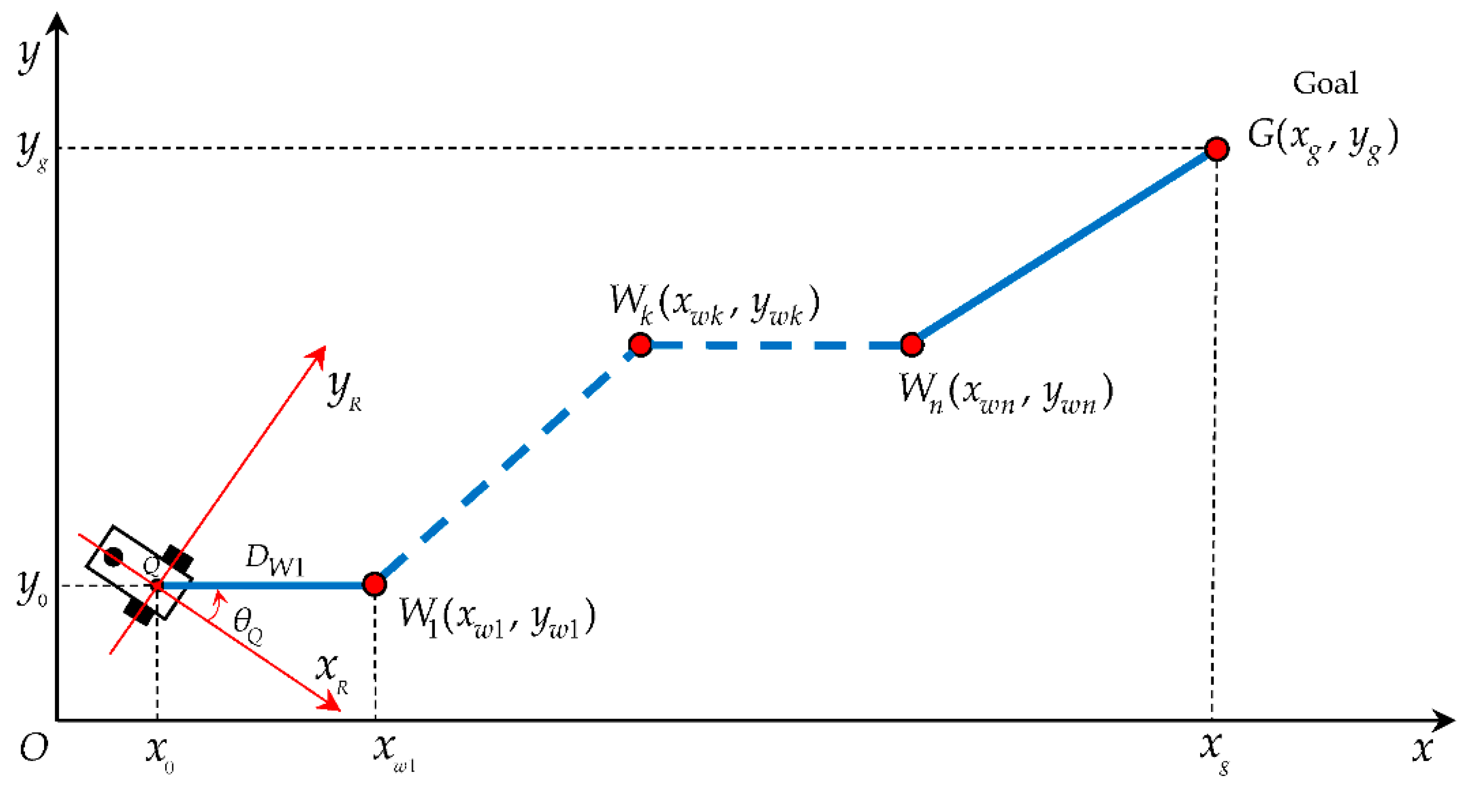
Without loss of generality, let us assume that the optimal path has been planned (in this case, the optimal path is optimized based on the A* algorithm with several waypoints [22], which is depicted in Figure 1); therefore the energy-efficient motion control problem of the DDWMR becomes the problem of designing an energy-efficient motion controller so that the robot can go to the goal through all waypoints efficiently.

In Figure 1, the differential drive wheeled mobile robot tracks the optimal path connecting the waypoints from the starting point (x₀, y₀) to the goal G(x_g, y_g) through several waypoints W_k(x_wk, y_wk), k = 2, 3, …, n − 1. (n is the total number of waypoints). The waypoints are determined by the planning layer of the robot (using the supervisory controller).

Navigating the DDWMR to the goal can be done with help of many different motion control algorithms. A general motion control system of the differential drive wheeled mobile robot is depicted in Figure 2. This scheme can be applied to most motion control algorithms to navigate the DDWMR to a given destination.

At first, an FLC is designed to navigate the DDWMR to the goal through all the waypoints sequentially. Then, a GA-based method is used to optimize the input and output membership functions for the FLC. To execute the optimization process of the FLC using the GA, as an optimizer of created Fitness Function (FF) based on simulated FLC performance, the “pymoo” library is employed.

A kinematic model and an energy model of the DDWMR are needed to design the optimal FLC. Thus, the following subsections will present them.

2.1. Kinematic Model of the Differential Drive Wheeled Mobile Robot

The geometry and kinematic parameters of the DDWMR are shown in Figure 3 [12].

In Figure 3, the DDWMR has the important parameters as follows: v is the robot linear velocity (m/s); θ is the robot orientation (rad); ω_r is the angular velocity of the right wheel (rad/s); ω_l is the angular velocity of the left wheel (rad/s); v_r is the linear velocity of the right wheel (m/s); v_l is the linear velocity of the left wheel (m/s); r is the radius of the right and the left wheels (m); b is the distance between the right and the left wheels (m); Q is the center of the axis between the right and the left wheels; G is the center of gravity of the DDWMR; a is the distance between Q and G (m).

Assuming that [12,29]:

-

The wheels are rolling without slipping,

-

The center of gravity G coincides with the point Q,

-

The guidance axis is perpendicular to the robot plane.

Based on Figure 3 and refer to [12,29], it is easy to get the kinematic model of the DDWMR as follows:

$$\{\begin{array}{l}\dot{x}=v\cos \theta \hfill \\ \dot{y}=v\sin \theta \hfill \\ \dot{\theta }=\omega \hfill \end{array}$$

(1)

2.2. Energy Model of the Differential Drive Wheeled Mobile Robot

The main energy losses of the DDWMR consist of the losses inside the motors, the kinetic energy losses, the losses due to friction, and the losses in the electronics [22,28]. The energy consumed by motors consists of two main parts, which are the energy transformed into robot kinetic energy and the energy to overcome traction resistance. In practice, the energy consumption is mainly transformed into robot kinetic energy.

For the design of an energy-efficient controller, it is necessary to have an appropriate energy model. To simplify the energy consumption model, only the kinetic energy losses of the robot have been considered. This simplification is based on the hypothesis that accelerations and decelerations change the kinetic energy of the robot body. The kinetic energy of the robot at any time is [12,22,28]

$$E_{\mathrm{kinetic}}=\frac{1}{2}m{\left[v(t)\right]}^2+\frac{1}{2}I{\left[\omega (t)\right]}^2$$

(2)

where m and I denote the mass and the moment of inertia of the differential drive wheeled mobile robot respectively; v and ω are the linear velocity and the angular velocity of the robot at time t.

When implementing movement of the DDWMR in the software, the discrete time is used. Thus, the kinetic energy of the robot at time t_i is calculated by Equation (3). The difference in kinetic energy between the two states is calculated by Equation (4).

$$E_{\mathrm{kinetic}(i)}=\frac{1}{2}m{\left[v(t_i)\right]}^2+\frac{1}{2}I{\left[\omega (t_i)\right]}^2$$

(3)

$$\mathsf{∆}{E}_{kinetic(i)}=E_{Kinetic(i)}-E_{Kinetic(i-1)}$$

(4)

where: i = 1, 2, 3, …, m (m is the number of sampling times).

The robot motion may include acceleration, deceleration, and moving with constant velocity. It is assumed that kinetic energy is not recuperated and stored in the battery; thus, every acceleration followed by deceleration leads to energy loss. To sum up all those energy differences, the state of the robot is inspected and the total energy consumption is calculated. Therefore, in the simulation, the total energy consumption of the DDWMR is calculated based on Equations (3) and (4), the kinetic energy changes in the deceleration phase are considered as a loss.

3. The Optimization of the Fuzzy Logic Controller Used for the Differential Drive Wheeled Mobile Robot

To carry out the full optimization process for the FLC, first, the initial FLC is created to navigate the DDWMR to the reference point. Then, the initial FLC will be optimized based on the GA to automatically tuning the parameters of the Membership Functions (MFs) for the FLC so that the energy consumption of the robot is minimum.

3.1. Design of the Initail Fuzzy Logic Controller

The movement of the differential drive wheeled mobile robot heading to the waypoint (W) is depicted in Figure 4.

From Figure 4 we get:

$$∆D=\sqrt{{\left(x_W-x_Q\right)}^2+{\left(y_W-y_Q\right)}^2}$$

(5)

$$∆\theta ={\theta }_R-{\theta }_W$$

(6)

$$\tan {\theta }_W=\frac{y_W-y_Q}{x_W-x_Q}$$

(7)

The ∆D is the distance and the ∆θ is the angle that is the difference between the current robot’s position and the waypoint’s position.

An FLC will be designed to guide the DDWMR from the current robot’s position Q(x_Q, y_Q) to the waypoint W(x_W, y_W). The general structure of a fuzzy logic controller is shown in Figure 5 [30,31,32].

The block diagram of the FLC used for the DDWMR is shown in Figure 6. For this FLC, two inputs (∆D and ∆θ) are used. Outputs of this FLC are the angular velocity of the left and the right wheels (ω_l, ω_r). These outputs are transformed into DDWMR inputs according to Equations (8) and (9).

$$v=\frac{1}{2}\left(v_r+v_l\right)$$

(8)

$$\dot{\theta }=\omega =\frac{1}{b}\left(v_r-v_l\right)$$

(9)

The FLC used for the DDWMR in this study is constructed as follows:

3.1.1. Selecting the Universes of Discourse

The universes of discourse are selected based on the robot parameters, the given path, the environment, etc. So, based on the parameters of the DDWMR and the given paths used in the experiments of this study, the authors have selected the universes of discourse as below:

The universe of discourse for input_1: ∆D (m) is 0 ≤ ∆D ≤ 10.

The universe of discourse for input_2: ∆θ (rad) is –π ≤ ∆θ ≤ π.

The universe of discourse for output_1: ω_r (rad/s) is 0 ≤ ω_r ≤ 30.

The universe of discourse for output_2: ω_l (rad/s) is 0 ≤ ω_l ≤ 30.

3.1.2. Constructing the Membership Functions and Rules

The triangular MFs are considered as a base form of the MFs. For each input and output, five MFs have been parametrized. The notations for the linguistic variables used to represent the MFs of input_1 are Very Close (VC), Close (C), Medium (M), Far (F), Very Far (VF). The notations for the linguistic variables used to represent the MFs of input_2 are Big Negative (BN), Negative (N), Zero (Z), Positive (P), Big Positive (BP). The notations for the linguistic variables used to represent the MFs of output_1 are Very Small Right (VSR), Small Right (SR), Medium Big Right (MBR), Big Right (BR), Very Big Right (VBR). The notations for the linguistic variables used to represent the MFs of output_2 are Very Small Left (VSL), Small Left (SL), Medium Big Left (MBL), Big Left (BL), Very Big Left (VBL). Based on the parameters of the robot, the given path, experiment, and experience, the parameters of all MFs are determined. These parameters are listed in

Table 1. Parameters used for inputs of the initial fuzzy logic controller.

The Distance Error ∆D (m)/The Angle Error ∆θ (rad)
Name	Notation	Parameters
Very Close/Big Negative	VC/BN	[0 0 2.5]/[–π –π –π/2]
Close/Negative	C/N	[0 2.5 5]/[–π –π/2 0]
Medium/Zero	M/Z	[2.5 5 7.5]/[–π/2 0 π/2]
Far/Positive	F/P	[5 7.5 10]/[0 π/2 π]
Very Far/Big Positive	VF/BP	[7.5 10 10]/[π/2 π π]

and

Table 2. Parameters used for outputs of the initial fuzzy logic controller.

The ωr (rad/s)/The ωl (rad/s)
Name	Notation	Parameters
Very Small Right/Left	VSR/VSL	[0 0 7.5]/[0 0 7.5]
Small Right/Left	SR/SL	[0 7.5 15]/[0 7.5 15]
Medium Big Right/Left	MBR/MBL	[7.5 15 22.5]/[7.5 15 22.5]
Big Right/Left	BR/BL	[15 22.5 30]/[15 22.5 30]
Very Big Right/Left	VBR/VBL	[22.5 30 30]/[22.5 30 30]

, and depicted in Figure 7.

Based on heuristics, the rules are selected for the FLC to generate each output (ω_l, ω_r) of the DDWMR in order to control the DDWMR to move to the waypoint. These rules are listed in

Table 3. The rules of the right wheel angular velocity.

	∆θ	BN	N	Z	P	BP
∆D
VC		VSR	SR	VSR	BR	VBR
C		VSR	SR	SR	BR	VBR
M		VSR	SR	MBR	BR	VBR
F		VSR	SR	BR	BR	VBR
VF		VSR	SR	VBR	BR	VBR

and

Table 4. The rules of the left wheel angular velocity.

	∆θ	BN	N	Z	P	BP
∆D
VC		VBL	BL	VSL	SL	VSL
C		VBL	BL	SL	SL	VSL
M		VBL	BL	MBL	SL	VSL
F		VBL	BL	BL	SL	VSL
VF		VBL	BL	VBL	SL	VSL

.

This FLC is used to control the DDWMR to move to the goal through all the waypoints sequentially. The next subsection will present the optimization process using the GA for this FLC to minimize the energy consumption of the robot.

3.2. Optimization of the Fuzzy Logic Controller Based on the Genetic Algorithm

The FLC design, the shape of the MFs, and the fuzzy rules are built entirely on heuristic definitions. Such the FLC design is complex, time-consuming, and its performances could be still poor. This section presents an optimization process defining the optimal parameters of the MFs for the FLC.

Currently, many researchers are using different heuristic algorithms that are not just bio-inspired but also based on physical laws [14], or using method cooperation in optimization process [33]. The computational methods inspired by biology are being used increasingly to deal with complex problems in robotics, engineering, computer science, etc. Among them, bio-inspired optimization is a term which covers a wide variety of optimization approaches. These methods are based on the principles of biological systems, such as bee colony optimization, bat algorithms, ant colony optimization, etc. Some other classes of optimization techniques are simulated annealing, neural network methods, and evolutionary algorithms including the GA [34]. As a method for the FLC optimization, the GA has been selected.

A typical GA cycle is shown in Figure 8. The GA is based on following operations: selection, genetic operations (crossover, mutation), and replacement [20,32,34,35].

3.2.1. Parameterization of the Membership Functions

Many types of the MFs have been used in fuzzy logic control systems, such as a triangular function, a trapezoidal function, a Gaussian function, etc. In the WMR field, the triangular and trapezoidal functions are applied more often than others [36]. Thus, in this study, the triangular function is selected to represent the MFs of the FLC because the triangular function is determined by just three parameters. Also, its evaluation is quite cheap, and the main advantage of the triangular function is the possibility to define it fully by just three parameters. Such a low number of parameters helps to lower the dimensionality of the optimization problem.

The triangular functions can be represented in different ways. A set of parameters defining these MFs is depicted in Figure 9.

In Figure 9, the (min, base1) is the set of parameters defining the 1st Membership Function (MF), the (base2, A1, base3) is the set of parameters defining the 2nd MF, the (base4, A2, base5) is the set of parameters defining the 3rd MF, the (base6, A3, base7) is the set of parameters defining the 4th MF, and the (base8, max) is the set of parameters defining the 5th MF. Thus, there is a total 11 parameters (base1, base2, A1, base3, …, A3, base7, base8). Here, min and max are the minimum and the maximum of the universe of discourse, respectively. A1–A3 and base1-base8 can take any value in the range [min; max] with the constraint (min < A1 < A2 < A3 < max).

The FLC has two inputs and two outputs as mentioned in the Section 3.1. Each input and output has five MFs described by 11 parameters, thus there is a total of 44 parameters for all inputs and outputs of the FLC. Here, the parameters of input_1 are (base1, base2, A1, base3, base4, A2, base5, base6, A3, base7, base8), the parameters of input_2 are (base9, base10, A4, base11, base12, A5, base13, base14, A6, base15, base16), the parameters of output_1 are (base17, base18, A7, base19, base20, A8, base21, base22, A9, base23, base24), the parameters of output_2 are (base25, base26, A10, base27, base28, A11, base29, base30, A12, base31, base32). These 44 parameters are encoded to 44 gens of each chromosome used in the GA, i.e., each chromosome represents all parameters of the input and output MFs. The structure of each chromosome can be represented as follows:

$$\mathrm{Chromosome}=\stackrel{44 \mathrm{gens}}{\overbrace{\underset{\mathrm{Input}\_1}{\underbrace{\mathrm{base}1, \dots ,\mathrm{base}8}}\underset{\mathrm{Input}\_2}{\underbrace{\mathrm{base}9, \dots ,\mathrm{base}16}}\underset{\mathrm{Outout}\_1}{\underbrace{\mathrm{base}17, \dots ,\mathrm{base}24}}\underset{\mathrm{Output}\_2}{\underbrace{\mathrm{base}25, \dots ,\mathrm{base}32}}}}$$

3.2.2. Fitness Functions Used for the Genetic Algorithm

In the GA, the FF is defined to obtain the FF value for each chromosome and to determine which one will be reproduced and taken into the next generation. So, with a particular chromosome, the FF returns a single numerical score, which is proportional to the ability of the chromosome (in this study, the score is a value of the energy consumption of the robot). The Equation (2) is used as the FF for the optimization process of the FLC based on the GA to minimize the energy consumption of the DDWMR.

To design an optimal FLC, first, an initial FLC is designed to navigate the DDWMR to the goal. Then, a GA process is executed in the Google Colab^® by using the Python language with the help of “pymoo” library to find the optimal parameters of the MFs.

It must be noticed that a single FF evaluation asks for running a complex simulation. Thus, running a full optimization process could need thousands of simulations. For such an extensive task, a quite powerful computer is needed. As FF evaluation could be done independently several FF computations can be run simultaneously. In this case, a computer cluster supporting distributed computation could help [37]. However, some kind of benchmarking and selection of several algorithms which promise effectiveness should be done [38].

The optimization process of the FLC with the help of the genetic algorithm is depicted in Figure 10.

The FLC is created according to the chromosome, which represents all parameters of the MFs, and consequently, its behavior is tested by a simulation process. Results of such simulation are transformed into fitness function value. Such a process of mapping from the proposed solution to the fitness function result allows the use of optimization methods. It is expected that the same mapping applied to the suboptimal solution gives the wanted FLC.

The “Tuning process (Genetic Algorithm)” block in Figure 10 are executed by the flow chart of the genetic algorithm depicted in Figure 11 as follows.

4. The Simulation Results and Discussion

4.1. Simulating and Collecting Results

4.1.1. Simulation Parameters

The parameters of the DDWMR used for the simulation in this study are taken from [12] that is shown in

Table 5. Parameters of the differential drive wheeled mobile robot.

Parameters	Value
Wheel’s radius (r)	0.0925 m
Distance between 2 driven wheels (b)	0.37 m
Mass of the robot (m)	9 kg
Moment of inertia of the robot (I)	0.16245 kgm2
Moment of inertia of the rotor (J)	0.01 kgm2/s2
Damping ratio (B)	0.1 Nms.
Electromotive force constant (K = Kt = Ke)	0.01 Nm/A
Electrical Resistance (Ra)	0.1 Ω
Electrical Inductance (La)	0.01 H
Start position of the robot on x axis (x0)	0 m
Start position of the robot on y axis (y0)	0 m
Start orientation of the robot (θ0)	45°

.

Several well-known effective motion controllers used to compare with the GA_FLC are the expert-based FLC [1], the Thoa-based FLC [6], the Circular-based controller [39], the energy-saving based algorithm introduced by Manas Chaudhari et al. [22,23], and the Mohammadian-based FLC_GA [40], the Robins Mathew-based controller [41,42]. Their coefficients are given in

Table 6. Coefficients of the several controllers.

No	Coefficients	Value
01	Circular-based controller
	Coefficient: gain	4.0
02	Robins Mathew-based controller
	Coefficient: k1	1.51
	Coefficient: k2	45.84
03	Chaudhari-based controller
	Minimal rotation radius: radius	0.1 m

.

Some given paths used for testing the robot motion control in this simulation are a zigzag path, a square path, a sharp turn path, a straightforward path, and a diamond-shaped path. These given paths are defined by several given points in a unit of a meter as in

Table 7. Parameters of the paths used for simulation.

Paths	Waypoints (x, y)
	1st Point	2nd Point	3rd Point	4th Point	5th Point
Zigzag path	(0, 0)	(10, 0)	(10, 10)	(20, 10)	(20, 20)
Square path	(0, 0)	(10, 0)	(10, 10)	(0, 10)	(0, 0)
Sharp turn path	(0, 0)	(10, 0)	(5, 10)	(15, 10)	-
Straightforward path	(0, 0)	(10, 2)	(20, 6)	-	-
Diamond-shaped path	(0, 0)	(10, −5)	(20, 0)	(10, 5)	(0, 0)

. In addition, a number eight-shaped path created by ($x=2+10\sin (\mathsf{\pi }t/30)$ and $y=1+5\sin (2\mathsf{\pi }t/30)$), and a circle path created by ($x=-8+8\cos (\mathsf{\pi }t/30)$ and $y=4+8\sin (\mathsf{\pi }t/30)$) are also used to test the ability tracking of the DDWMR when using the GA_FLC.

The rules and the MFs of the several used fuzzy logic controllers are as follows:

For the initial FLC: the rules are shown in Table 3 and Table 4. The parameters of the MFs are shown in Table 1 and Table 2.

For the expert-based FLC: the rules are shown in Table 1 of [1]. The parameters of the MFs are shown in

Table 8. Parameters for inputs of the expert-based FLC.

The Distance Error ∆D (m)/The Angle Error ∆θ (rad)
Name	Notation	Parameters
Very Close/Very Big Negative	VC/VBN	[0 0 1]/[–π –π –π/2]
Near Close/Big Negative	NC/BN	[0 1 2]/[–π –π/2 –π/4]
Close/Negative	C/N	[1 2 3]/[–π/2 –π/4 0]
Medium/Zero	M/Z	[2 3 5]/[– π/4 0 π/4]
Near Far/Positive	NF/P	[3 5 7]/[0 π/4 π/2]
Far/Big Positive	F/BP	[5 7 10]/[π/4 π/2 π]
Very Far/Very Big Positive	VF/VBP	[7 10 10]/[π/2 π π]

and

Table 9. Parameters for outputs of the expert-based FLC.

The ωr (rad/s)/The ωl (rad/s)
Name	Notation	Parameters
Very Small Right/Left	VSR/VSL	[0 0 5]/[0 0 5]
Small Right/Left	SR/SL	[0 5 10]/[0 5 10]
Near Medium Big Right/Left	NMBR/NMBL	[5 10 15]/[5 10 15]
Medium Big Right/Left	MBR/MBL	[10 15 20]/[10 15 20]
Near Big Right/Left	NBR/NBL	[15 20 25]/[15 20 25]
Big Right/Left	BR/BL	[20 25 30]/[20 25 30]
Very Big Right/Left	VBR/VBL	[25 30 30]/[25 30 30]

.

For the Thoa-based FLC: the rules are shown in Table 2 and Table 3 of [6]. The parameters of the MFs are used the same as the MFs of the initial FLC shown in Table 1 and Table 2.

For the Mohammadian-based FLC_GA controller: based on the Mohammadian method [40], the input MFs and the rules can be used the same as the initial FLC. Mohammadian et al. have only optimized output MFs. According to them, for optimization of the MFs it only need to optimize the overlaps between the output MFs [40]. The output MFs used for the Mohammadian-based FLC_GA controller are represented in Figure 12. In Figure 12, B1–B4 are overlaps between the output MFs which need to tune. The values of these overlaps are selected in the range [0 to 7.5].

For all used controllers here, based on the parameters of the DDWMR and parameters of the given paths, the linear velocity (v) is limited to the range [0 m/s to 2.0 m/s], and the angular velocity (ω) is limited to the range [–0.75 rad/s to 0.75 rad/s] because the movement of a mobile robot will be directly affected by the speed that its actuator can provide. If the provided velocity is too large, it will cause some difficulty in tracking, a high energy loss, and a big tracking error. Conversely, if the provided velocity is too small, the robot will move too slowly, which may affect its performances.

4.1.2. Simulation Open-Course Code

The simulation program of this experiment is published as an open-source code for all readers. This simulation has been developed by employing of the Google Colab^® and the Python language. The open-source code has been published on Code Ocean (https://doi.org/10.24433/CO.1867832.v1) (accessed on 2 March 2021) [43], it also has been stored in Colaboratory (https://colab.research.google.com/drive/17FUnDR7XNjMsDOFrXfnBNWffqXYntEjF?usp=sharing) (accessed on 3 May 2021), and in GitHub^® (https://github.com/vanthuanhvhq/GA_FLC) (accessed on 4 May 2021) so that readers can browse, view, run and experiment with the codes. However, to run this simulation program faster, users should setup their own cluster then replace the URL address with theirs. Otherwise they will experience a long run. This program consists of several sections, which have been explained in the simulation program.

4.1.3. Collecting Results

Firstly, the zigzag path will be used to optimize the FLC by using the GA. Running the simulation with its default configuration and setting up the population size at 50, all the results of these experiments in 200th generation for the zigzag path are shown in Figure 13 and Figure 14 and

Table 10. Energy consumption and travel distance of the robot when the robot tracks the zigzag path based on optimizing by genetic algorithm. Bold values are the best in the appropriate column.

Generation	Energy Consumption (J)	Travel Distance (m)
30	15.93	48.53
50	10.18	50.42
100	8.50	46.27
150	8.49	46.07
200	8.47	46.10

and

Table 11. Energy consumption and travel distance of the robot when the robot tracks the zigzag path by the different controllers. Bold values are the best in the appropriate column.

Controllers	Energy Consumption		Travel Distance
	E (J)	E (%)	s (m)	s (%)
Circle-based controller	17.80	210.15	52.77	122.90
Mathew-based controller	70.14	828.10	42.94	100.00
Chaudhari-based controller	17.91	211.45	52.62	122.54
Thoa-based controller	69.30	818.19	51.90	120.87
Expert-based controller	69.52	820.78	45.25	105.38
Mohammadian-FLC	62.49	737.78	46.15	107.46
Proposed GA_FLC	8.47	100.00	46.10	107.36

. Then this GA_FLC will be used to evaluate its control performance when the differential wheeled mobile robot tracks the other paths. The results are shown in Figure 15 and in

Table 12. Energy consumption and travel distance of the robot when the robot tracks the square path by the different controllers. Bold values are the best in the appropriate column.

Controllers	Energy Consumption		Travel Distance
	E (J)	E (%)	s (m)	s (%)
Circle-based controller	17.80	210.15	45.80	106.66
Mathew-based controller	70.11	827.75	42.94	100.00
Chaudhari-based controller	17.90	211.33	46.19	107.57
Thoa-based controller	69.11	815.94	44.09	102.68
Expert-based controller	69.51	820.66	43.12	100.42
Mohammadian-FLC	61.83	730.00	43.00	100.14
Proposed GA_FLC	8.47	100.00	43.23	100.68

,

Table 13. Energy consumption and travel distance of the robot when the robot tracks the sharp turn path by the different controllers. Bold values are the best in the appropriate column.

Controllers	Energy Consumption		Travel Distance
	E (J)	E (%)	s (m)	s (%)
Circle-based controller	17.76	209.68	43.82	129.42
Mathew-based controller	53.04	626.21	33.86	100.00
Chaudhari-based controller	17.85	210.74	45.09	133.17
Thoa-based controller	51.91	612.87	45.93	135.65
Expert-based controller	52.25	616.88	37.30	110.16
Mohammadian-FLC	51.53	608.38	38.32	113.17
Proposed GA_FLC	8.47	100.00	39.93	117.93

,

Table 14. Energy consumption and travel distance of the robot when the robot tracks the straightforward path by the different controllers. Bold values are the best in the appropriate column.

Controllers	Energy Consumption		Travel Distance
	E (J)	E (%)	s (m)	s (%)
Circle-based controller	17.66	211.24	21.39	101.18
Mathew-based controller	18.89	225.96	21.36	101.62
Chaudhari-based controller	17.76	212.44	21.39	101.76
Thoa-based controller	38.95	465.91	21.08	100.29
Expert-based controller	35.37	423.09	21.03	100.05
Mohammadian-FLC	35.76	427.75	21.02	100.00
Proposed GA_FLC	8.36	100.00	21.29	101.29

and

Table 15. Energy consumption and travel distance of the robot when the robot tracks the diamond-shaped path by the different controllers. Bold values are the best in the appropriate column.

Controllers	Energy Consumption		Travel Distance
	E (J)	E (%)	s (m)	s (%)
Circle-based controller	17.80	207.94	51.29	108.57
Mathew-based controller	52.21	609.93	47.24	100.00
Chaudhari-based controller	17.92	209.35	51.03	108.02
Thoa-based controller	69.07	806.89	50.39	106.67
Expert-based controller	69.53	812.27	48.49	102.65
Mohammadian-FLC	70.88	828.04	48.30	102.24
Proposed GA_FLC	8.56	100.00	49.84	105.50

. The convergence of the FF value is shown in Figure 16.

4.2. Discussion

4.2.1. When the Robot Tracks the Zigzag Path

For the optimization of the FLC with the use of the GA, the population size is set to 50 and the number of generations to 200. Those parameters have been found as a good trade-off between the fast optimization process and behavior of the resulted FLC. Experiments show that a smaller population leads to a worse FLC. Specifically, when using the population size is 10 and 45, the energy consumption increases 257.6% and 19.5%, respectively in comparison with the case of using the population size is 50. These are quite high energy consumptions. In contrast, when using the population size is greater than 50, that leads to a slower optimization process, and the energy consumption also increases in comparison with the case of using the population size 50. For example, the processing time increases 21.1% and the energy consumption also increases 15.6% when using the population size is 55 in comparison with the case of using the population size is 50.

Figure 16 and the simulation results clearly indicate that the value of the fitness function is rapidly reduced during the optimization process (from the 1st generation to the 40th generation). Then the value of this fitness function is slightly decreased from the 41st generation to the 53rd generation. From the 54th generation onwards the value of the fitness function converges to E = 8.47 J and remains at this value. As this experiment is based on random behavior and it has been executed repeatedly, it can be concluded that the fitness function has converged and reached a stable suboptimal value.

Table 10 shows the values of the energy consumption and the travel distance collected after the different generations (30th, 50th, 100th, 150th, 200th), when the optimization of the FLC using the genetic algorithm to track the zigzag path with the size of the initial population is 50. Table 10 shows that the minimum value of the energy consumption has been obtained at the 200th generation (E = 8.47 J), and the smallest value of the travel distance has been obtained at the 150th generation (s = 46.07 m). However, this study mainly aims to minimize the energy consumption. Thus, the best results (in terms of fitness function value) which have been obtained are (E = 8.47 J) and (s = 46.10 m) at the 200th generation.

Figure 13 and Table 11 serve as the base for a comparison between the proposed controller (GA_FLC) with other previous published controllers. When the differential drive wheeled mobile robot is controlled by the GA_FLC to track the zigzag path, the energy consumption of the robot is much lower than the energy consumption of the robot controlled by any other used controller. In this case, the GA_FLC has saved more than 110.1% energy in comparison with the other controllers.

In addition, Figure 13c,d also show that the linear velocity and the angular velocity of the robot controlled by the Circle-based controller, the Mathew-based controller, the Chaudhari-based controller, the Thoa-based controller, the Expert-based controller, and the Mohammadian-FLC have oscillated over time, which has led to the vibrations and jerks of the robot. However, this problem has been fixed quite well when the GA_FLC is used. Figure 13c shows that when the GA_FLC is used, the linear velocity is almost not changed, i.e., the linear velocity of the robot is almost constant during the movement, even when the robot moves through the corner. Moreover, Figure 13d also shows that the angular velocity of the robot controlled by the GA_FLC only changes the value at the time when the robot turns at each corner of the path, i.e., the robot only changes its orientation at the corner of the path. Therefore, the issues about the robot vibration and the robot jerk have been solved quite well by the GA_FLC.

Besides, Figure 13a and Table 11 show that when controlling the differential drive wheeled mobile robot by the GA_FLC, the tracking error is quite small. This error is the smallest in all, except the error tracking of the robot when it is controlled by the Mathew_based controller. Furthermore, Figure 13e,f also indicate that the energy consumption of the DDWMR when it is controlled by GA_FLC is the smallest and it increases insignificantly from about 2 s to 40 s.

As mentioned previously, the optimization of the FLC using the GA based on minimizing energy consumption criterion would be the prime objective of this study, thus from the analyses above, it can be concluded that the proposed controller (GA_FLC) is the best one. In other words, the GA_FLC is much better than others in terms of energy-saving and the other performances of motion control are still good.

4.2.2. When the Robot Tracks the Other Different Paths

In order to investigate operating ability of the GA_FLC, it has been used to control the DDWMR to move in several typical different paths. In this case, the DDWMR is controlled by the GA_FLC (optimized and taken from the previous experiment) to track the square path, the sharp turn path, the straightforward path, and the diamond-shaped path sequentially. Figure 15a–d and Table 12, Table 13, Table 14 and Table 15 indicate that the performance of the motion control is still good when the robot is controlled by the GA_FLC compared to the others in all given paths. Specifically, 110.2%, 109.7%, 110.3%, and 107.9% reduction of the energy consumption was achieved using the proposed method compared to the best of six alternatives studied when the robot tracks the square path, the sharp turn path, the straightforward path, and the diamond shaped path, respectively. Especially, the limitations of the other controllers such as the vibration and the jerk have been solved by the GA_FLC. So, it can be also concluded that the GA_FLC is the best controller for the differential drive wheeled mobile robot on the different given paths.

In addition, Figure 15e,f indicate that the robot still tracks the number eight-shaped path and the circle path tightly. In these cases, the energy consumption of the differential drive wheeled mobile robot is also quite low (E = 8.73 J for the number eight-shaped path, and E = 8.75 J for the circle path).

4.3. Future Work

In a future research, the work will be focused on: (1) both the energy consumption and the travel distance will be taken into account when optimizing the FLC. (2) both the parameters of all MFs and the rule base will be considered to optimize the FLC. (3) robustness of the proposed GA_FLC will be analyzed to clarify the control performance of the robot. The robustness of the GA_FLC is a complex and difficult issue, which needs to be thoroughly addressed. So, this issue will be comprehensively presented in our future work. For more detail about the robustness of an FLC, refer to [44,45,46].

5. Conclusions

In this paper, the FLC has been introduced and successfully applied for the DDWMR control for robot movement on the given path. However, it is too complex and time-consuming to manually search for the proper parameters of the MFs, and its performances of motion control are still poor. To tackle such problems, an optimal FLC (GA_FLC) has been found with the use of the GA and the minimum energy consumption criterion. In many studies, scientists have only optimized the output MFs. However, in this study, the GA automatically tunes all the parameters of input/output MFs of the FLC. Such an approach leads to fast and effective tuning. For the optimal parameters’ identification of the MFs for the FLC, the zigzag path has been used in the optimization process at first. The fitness function has been derived from the energy consumption and after that minimized. Also, the length of the traveled path has been considered. Finally, the performance of suboptimal FLC has been tested on the benchmark paths and its results have been compared to the results of several controllers based on another approaches. The comparisons have shown that the GA_FLC is much better than all used well-known controllers in terms of energy consumption while the other performances of the motion parameters are still good.

To keep all experiments reproducible, the GA_FLC and several well-known controllers including the Circle-based controller, the Mathew-based controller, the Chaudhari-based controller, the Thoa-based controller, the Expert-based controller, and the Mohammadi-based FLC controllers have been successfully implemented in the Google Colab^® by using the Python language and made freely available for all the readers who are interested in them.

References

1. Faisal, M.; Algabri, M.; Abdelkader, B.M.; Habib, D.; Mohamad, M.A.R. Human expertise in mobile robot navigation. IEEE Access 2017, 6, 1694–1705. [Google Scholar] [CrossRef]
2. Abdullah, N.A. Fuzzy logic based real time go to goal controller for mobile robot. IJCA 2020, 176, 32–36. [Google Scholar] [CrossRef]
3. Lukuman, A.Y.; Ado, D.I. Fuzzy logic control of goal-seeking 2-wheel differential mobile robot using unicycle approach. In Proceedings of the IEEE International Conference on Automatic Control and Intelligent Systems (I2CACIS), Selangor, Malaysia, 29 June 2019; pp. 300–304. [Google Scholar] [CrossRef]
4. Meshram, R.B. Motion control of wheeled mobile robots using fuzzy logic. IJRTE 2013, 2, 89–93. [Google Scholar]
5. Abdelwahab, M.; Parque, V.; Elbab, A.M.R.F.; Abouelsoud, A.A.; Sugano, S. Trajectory tracking of wheeled mobile robots using Z-number based fuzzy logic. IEEE Access 2020, 8, 18426–18441. [Google Scholar] [CrossRef]
6. Thoa, T.M.; Cosmin, C.; Keyser, D.R.; Trung, D.T.; Thich, V. MIMO fuzzy control for autonomous mobile robot. J. Autom. Control Eng. 2016, 4, 65–70. [Google Scholar] [CrossRef] [Green Version]
7. Shuying, P.; Wuxi, S. Adaptive fuzzy output feedback control of a nonholonomic wheeled mobile robot. IEEE Access 2018, 6, 43414–43424. [Google Scholar] [CrossRef]
8. Ran, Z.; Dong, H.L.; Hong, K.L. Mobile robot navigation using optimized fuzzy controller by genetic algorithm. IJFIS 2015, 15, 12–19. [Google Scholar] [CrossRef]
9. Prases, K.M.; Dayal, R.P. Navigation of autonomous mobile robot using adaptive network based fuzzy inference system. Mech. Sci. Technol. 2014, 28, 2861–2868. [Google Scholar] [CrossRef]
10. Panati, S.; Kil, T.C. Adaptive network fuzzy inference system based navigation controller for mobile robot. Front. Inf. Technol. Electron. Eng. 2019, 20, 141–151. [Google Scholar] [CrossRef]
11. Shubhasri, K.; Dayal, R.P.; Deepak, B.B.V.L. Fuzzy-neuro based navigational strategy for mobile robot. IJSER 2012, 3, 1–6. Available online: http://citeseerx.ist.psu.edu/viewdoc/summary?doi=10.1.1.302.2880 (accessed on 2 May 2021).
12. Stefek, A.; Thuan, V.P.; Krivanek, V.; Lam, K.P. Energy comparison of controllers used for a differential drive wheeled mobile robot. IEEE Access 2020, 8, 170915–170927. [Google Scholar] [CrossRef]
13. Claudio, U.; John, K.; Johanna, A. Design and evaluation of a new fuzzy control algorithm applied to a manipulator robot. Appl. Sci. 2020, 10, 7482. [Google Scholar] [CrossRef]
14. Cinthia, P.; Fevrier, V.; Oscar, C. An adaptive fuzzy control based on Harmony search and its application to optimization. In Nature-Inspired Design of Hybrid Intelligent Systems; Springer: Berlin/Heidelberg, Germany, 2017; Volume 667, pp. 269–283. [Google Scholar] [CrossRef]
15. Dongkyoung, C.; Junseok, B. Adaptive fuzzy output feedback simultaneous posture stabilization and tracking control of wheeled mobile robots with kinematic and dynamic disturbances. IEEE Access 2020, 8, 228863–228878. [Google Scholar] [CrossRef]
16. Mauricio, B.; Douglas, W.B.; Nardenio, A.M. A robust adaptive fuzzy variable structure tracking control for the wheeled mobile robot: Simulation and experimental results. Control Eng. Pract. 2017, 64, 27–43. [Google Scholar] [CrossRef]
17. Herrera, F.; Lozano, M.; Verdegay, J.L. Tuning fuzzy logic controllers by genetic algorithms. Int. J. Approx. Reason. 1995, 12, 299–315. [Google Scholar] [CrossRef] [Green Version]
18. Kumarasamy, K.S. Single robot motion planning using fuzzy-genetic technique. Control Intell. Syst. J. 2010, 1, 1–8. [Google Scholar]
19. Lei, M.; Guan, Z.; Yang, S. Mobile robot fuzzy control optimization using genetic algorithm. Artif. Intell. Eng. 1996, 10, 293–298. [Google Scholar] [CrossRef]
20. Ahmet, A.; Mehmet, K. Determination of fuzzy logic membership functions using genetic algorithms. Fuzzy Sets Syst. 2001, 118, 297–306. [Google Scholar] [CrossRef]
21. Karim, B.; Zhu, Q. Genetic fuzzy logic control technique for a mobile robot tracking a moving target. IJCSI 2013, 10, 607–613. [Google Scholar]
22. Liu, S.; Sun, D. Minimizing Energy Consumption of Wheeled Mobile Robots via Optimal Motion Planning. IEEE/ASME Trans. Mechatron. 2014, 19, 401–411. [Google Scholar] [CrossRef]
23. Chaudhari, M.; Leena, V.; Rangan, B. Towards optimal computation of energy optimal trajectory for mobile robots. In Proceedings of the Third International Conference on Advances in Control and Optimization of Dynamical Systems, Kanpur, India, 13–15 March 2014; pp. 82–87. [Google Scholar] [CrossRef]
24. Seilla, A.; Shofuro, A.; Paramadina, S.; Rizki, A.P.; Denny, D. Efficient energy consumption for indoor mobile robot prototype under illumination. MATEC Web Conf. 2018, 197, 1–4. [Google Scholar] [CrossRef]
25. Gurguze, G.; Turkoglu, I. Energy management techniques in mobile robot. IJEPE 2017, 11, 1085–1093. [Google Scholar] [CrossRef]
26. Mauricio, F.J.; Sedat, D.; Lino, M. Generation of energy optimal speed profiles for a differential drive mobile robot with payload on straight trajectories. In Proceedings of the 2020 IEEE International Symposium on Safety, Security, and Rescue Robotics (SSRR), Abu Dhabi, United Arab Emirates, 4–6 November 2020; pp. 136–141. [Google Scholar] [CrossRef]
27. Minghan, W.; Volkan, I. Coverage path planning under the energy constraint. In Proceedings of the 2018 IEEE International Conference on Robotics and Automation (ICRA), Brisbane, Australia, 21–25 May 2018; pp. 368–373. [Google Scholar] [CrossRef]
28. Mudasser, W.; Fernando, R.; Adel, E.S. Energy modeling of differential drive robots. In Proceedings of the IEEE SoutheastCon 2015, Fort Lauderdale, FL, USA, 9–12 April 2015; pp. 1–6. [Google Scholar] [CrossRef]
29. Tzafestas, S.G. Introduction to Mobile Robot Control, 1st ed.; Elsevier: Amsterdam, The Netherlands, 2014; pp. 137–317. [Google Scholar]
30. Zhang, P. Advanced industrial control technology. In Advanced Industrial Control Technology, 1st ed.; Elsevier: Amsterdam, The Netherlands, 2010; pp. 257–305. ISBN 9781437778076. [Google Scholar] [CrossRef]
31. Nandan, R. An Intelligent Approach to Positive Target Identification. In Soft Computing and Intelligent Systems, 1st ed.; Naresh, K.S., Madan, M.G., Eds.; Academic Press Series in Engineering; Elsevier: Amsterdam, The Netherlands, 2000; pp. 549–570. ISBN 978-0-12-646490-0. [Google Scholar] [CrossRef]
32. Zilouchian, A.; Jamshidi, M. Intelligent Control Systems Using Soft Computing Methodologies, 1st ed.; Ali, Z., Mo, J., Eds.; CRC Press: Boca Raton, FL, USA, 2001; pp. 211–234. ISBN 9780849318757. [Google Scholar]
33. Krupka, Z.; Stefek, A. Method cooperation in optimization process. In Proceedings of the 13th Mechatronika 2010, Trencianske Teplice, Slovakia, 2–4 June 2010; pp. 21–23. [Google Scholar]
34. Deepak, R.; Kirti, T. Bio-inspired optimization techniques: A critical comparative study. ACM SIGSOFT Softw. Eng. Notes 2013, 38, 1–7. [Google Scholar] [CrossRef]
35. Wahde, M. Evolutionary algorithms. In Biologically Inspired Optimization Methods, 1st ed.; WIT Press: Göteborg, Sweden, 2008; pp. 35–98. [Google Scholar]
36. Mehdi, Z.; Ebrahim, A.; Mehdi, F. A Review on optimization of fuzzy controller parameters in robotic applications. IETE J. Res. 2020, 1–10. [Google Scholar] [CrossRef]
37. Stefek, A. Distributed optimization—Concepts, ideas and solutions. Croat. J. Educ. 2013, 14, 161–167. [Google Scholar]
38. Stefek, A. Benchmarking of heuristic optimization methods. In Proceedings of the 14th International Conference Mechatronika, Trencianske Teplice, Slovakia, 1–3 June 2011; pp. 68–71. [Google Scholar] [CrossRef]
39. Stefek, A.; Krivanek, V.; Yves, T.B.; Jean, M. Differential drive robot: Spline-based design of circular path. In Dynamical Systems: Theoretical and Experimental Analysis; Springer Proceedings in Mathematics & Statistics; Springer: Berlin/Heidelberg, Germany, 2016; Volume 182, pp. 331–342. [Google Scholar]
40. Mohammadian, M.; Stonier, R.J. Tuning and optimisation of membership functions of fuzzy logic controllers by genetic algorithms. In Proceedings of the 3rd IEEE International Workshop on Robot and Human Communication, Nagoya, Japan, 18–20 July 1994; pp. 356–361. [Google Scholar] [CrossRef]
41. Kanayama, Y.; Kimura, Y.; Miyazaki, F.; Noguchi, T. A stable tracking control method for a non-holonomic mobile robot. In Proceedings of the IROS ‘91:IEEE/RSJ International Workshop on Intelligent Robots and Systems, Osaka, Japan, 3–5 November 1991; pp. 1236–1241. [Google Scholar] [CrossRef]
42. Robins, M.; Somashekhar, S.H. Development of waypoint tracking controller for differential drive mobile robot. In Proceedings of the International Conference on Control, Decision and Information Technologies (CoDIT), Paris, France, 23–26 April 2019; pp. 1121–1126. [Google Scholar] [CrossRef]
43. Stefek, A.; Thuan, V.P.; Krivanek, V.; Lam, K.P. Optimization of Fuzzy Logic Controller Used for a Differential Drive Wheeled Mobile Robot [Source Code]. Code Ocean 2021. [Google Scholar] [CrossRef]
44. Hosseinzadeh, M.; Sadati, N.; Zamani, I. H∞ disturbance attenuation of fuzzy large-scale systems. In Proceedings of the International Conference on Fuzzy Systems, Taipei, Taiwan, 27–30 June 2011; pp. 2364–2368. [Google Scholar] [CrossRef]
45. Zhang, J.; Chen, W.H.; Lu, X. Robust fuzzy stabilization of nonlinear time-delay systems subject to impulsive perturbations. Commun. Nonlinear Sci. Numer. Simul. 2020, 80, 1–13. [Google Scholar] [CrossRef]
46. Yi, S.Y.; Chung, M.J. Robustness of fuzzy logic control for an uncertain dynamic system. IEEE Trans. Fuzzy Syst. 1998, 6, 216–225. [Google Scholar] [CrossRef]
Figure 1. The differential drive wheeled mobile robot tracks the optimal path with several waypoints.
Applsci 11 06023 g001
Figure 2. A general mobile robot motion control system.
Applsci 11 06023 g002
Figure 3. Geometry of a differential drive wheeled mobile robot.
Applsci 11 06023 g003
Figure 4. The differential drive wheeled mobile robot and the waypoint parameters.
Applsci 11 06023 g004
Figure 5. The fuzzy logic controller block diagram.
Applsci 11 06023 g005
Figure 6. The block diagram of the fuzzy logic controller used for the differential drive wheeled mobile robot.
Applsci 11 06023 g006
Figure 7. (a) The membership functions of the distance error; (b) The membership functions of the angle error; (c) The membership functions of the right wheel angular velocity; (d) The membership functions of the left wheel angular velocity.
Applsci 11 06023 g007
Figure 8. The genetic algorithm cycle block diagram.
Applsci 11 06023 g008
Figure 9. The triangular membership functions with their parameters.
Applsci 11 06023 g009
Figure 10. The optimization process used for optimization of the fuzzy logic controller.
Applsci 11 06023 g010
Figure 11. The flow chart of the used genetic algorithm.
Applsci 11 06023 g011
Figure 12. The output membership functions used for the Mohammadian-based FLC_GA.
Applsci 11 06023 g012
Figure 13. Analysis of the simulation results for the zigzag path. (a) The zigzag path tracking of the robot; (b) The robot’s travel distance over time when the robot tracks the zigzag path; (c) The robot’s linear velocity over time when the robot tracks the zigzag path; (d) The robot’s angular velocity over time when the robot tracks the zigzag path; (e) The robot’s kinetic energy loss over time when the robot tracks the zigzag path; (f) The zoom of the robot’s kinetic energy loss over time when the robot tracks the zigzag path.
Applsci 11 06023 g013
Figure 14. The membership function used for the zigzag path. (a) The distance membership functions before tuning; (b) The distance membership functions after tuning; (c) The angle membership functions before tuning; (d) The angle membership functions before tuning; (e) The output _1 (Omega_R) membership functions before tuning; (f) The output _1 (Omega_R) membership functions after tuning; (g) The output _2 (Omega_L) membership functions before tuning; (h) The output _2 (Omega_L) membership functions after tuning.
Applsci 11 06023 g014
Figure 15. Analysis of the simulation results for the other paths. (a) The square path tracking of the robot; (b) The sharp turn path tracking of the robot; (c) The straightforward path tracking of the robot; (d) The diamond-shaped path tracking of the robot; (e) The number eight-shaped path tracking of the robot when it is controlled by the GA_FLC; (f) The circle path tracking of the robot when it is controlled by the GA_FLC.
Applsci 11 06023 g015
Figure 16. The convergence of energy fitness function.
Applsci 11 06023 g016