1. Introduction
In underground mining, we observe a dynamic growth in the development of monitoring and analytics, both in the case of stationary and mobile assets. For an LHD machine (Load—Haul—Dump vehicle), the main directions of analytical development are primarily related to the identification of operating cycles, efficiency assessment [
1,
2,
3], technical diagnostics [
4], identification of dynamic overloads, road condition classification [
5], assessment of the driving style of operators, assessment of road conditions [
6], and optimization of production [
7]. Tracking the workflow of the mining fleet is a key challenge for an underground mine. Taking into account the number of operational contexts, especially the external factors influencing the operational parameters of mining machines, the location of machines in underground mining excavations is crucial for data analysis from monitoring systems. The solutions available on the market are usually based on GPS and relate to opencast mines. In the literature, we can find several works on the location of assets in underground excavation. Oftentimes, they are based on inertial measurements, odometry, or RFID (Radio-frequency identification) technology. Inertial navigation systems for underground mining have been developed since the mid-1990s [
8]. This type of navigation was usually developed with the automatization of LHD machines for strictly defined conditions of deposit exploitation [
9,
10,
11]. In practice, the development of inertial navigation for universal use in an underground mine is difficult to achieve, among others due to the phenomenon of gyroscope drift and several disturbances, especially in the magnetometer readings. Such systems are usually based on RFID technology, in which the key is to recognize the entry or exit of a machine from a given mine zone. In practice, gates are most often installed at intersections, and the proposed solution ensures the identification of the machine passing through the intersection, its direction, and the turning angle itself. In the case of exploitation of the deposit based on a room-and-pillar system where the layout of the excavations has a Manhattan structure, achieving precision at the crosscut level is sufficient. The main problem is related to the constant expansion of the extensive communication infrastructure, which is certainly neither cheap nor easy to maintain.
In this article, we present a simple and inexpensive approach to the vehicle turn detection problem based on inertial sensors. The proposed algorithm provides the identification of the time moment of the turning maneuver, its direction, and approximate angle. The turn identification algorithm can find a wide range of applications. First of all, it can be used to recognize and correct the LHD motion path based on the gyro integral. In [
12], the authors proposed a localization model based on IMU (Inertial Measurement Unit) sensors and a digital map for a room-and-pillar system on the example of KGHM’s underground copper ore mine. After minor modifications, the turn detection algorithm can be a significant simplification of the model of the machine location on the digital map. Additionally, identifying the machine’s turns at crossroads is particularly important when assessing the operator’s driving style. It is necessary to check the operator’s behavior, especially if they have followed the manufacturer’s recommendations in terms of driving speed. Another application example is the analysis of dynamic overloads and stresses occurring during the turning maneuver in the reliability tests of structural nodes. After the detection of turns, the signal from the IMU coming from these specific signal fragments can be utilized, for example in the problem of driver classification and driving style recognition [
13,
14]. In those cases usually, the information about turns is obtained (a) from the steering sensor mounted on the steering wheel, which is not available in our case, (b) is read from GPS, which does not work in an underground mine, or (c) in addition to a gyroscope, by utilizing magnetometer data (to reduce the drift problem), which readings are unreliable in mines. Therefore, there is a need to develop a separate, reliable turn-detection method, possible to be used in the difficult conditions of an underground mine.
2. Description of Research
As mentioned, the main purpose of our research was the detection of machine turning moments (understood as a moment in time) while driving in an underground mine. If acquired, this information could be useful in many other algorithms, for example in the underground localization problem. Unfortunately, collecting data about vehicle turns with sufficient accuracy is a challenging task, mainly due to the drift that the gyroscope readings are burdened with. In standard conditions, such as in the case of drones, the IMU sensors are constantly corrected via the sensor fusion algorithms with other information sources such as GPS; however, in the case of underground mines, such methods either only partially solve the problem or are unavailable. This is why our research mainly focuses on an algorithmic approach to such an environment with the use of machine learning.
The machine used for the research was a haul truck operating in the KGHM Polska Miedź S.A. mines located in Poland. Haul trucks are used to haul material, including hauling the ore from mining faces to department dumping points, which are secured with grids. A single haulage cycle encompasses four basic procedures: (a) loading of the cargo box of the machine at the mining face, (b) hauling material to the dumping point, (c) dumping material, (d) returning the machine to the loading zone at the mining face. There are few types of haul trucks operating in KGHM’s mines, varying mostly in the cargo box capacities. The experiments from which the data are analyzed in this article were conducted on a common haul truck, of which the model should not affect the proposed method results. This type of wheeled vehicle consists of a tractor unit and a cargo box both connected by a joint. The vehicle and IMU mounting location on the machine, as well as a fragment of underground excavation, is presented in
Figure 1.
The measuring device used in the experiments was x-io Technologies NGIMU (New Generation IMU—
Figure 2A) with 10 DoF (Degrees of Freedom), which includes a triple-axis: gyroscope, accelerometer, magnetometer, and single-axis humidity and barometric pressure sensor. The range of the used gyroscope is equal to 2000 deg/s, and the accelerometer range is 16 g. The maximum sampling rate of the device is 400 Hz with a resolution equal to 16 bit. In addition, the machine itself measures some of its parameters, such as speed, engine speed, or hydraulic pressure, using an on-board monitoring system called SYNAPSA. These variables are being sampled with a frequency of 100 Hz, but later, at the stage of data storage in the repository, they are averaged to 1 Hz.
Two NGIMU units were mounted on the haul truck with the use of a specially developed steel housing, ensuring simple and inflexible assembly and protection against mechanical damage and harsh environmental conditions (
Figure 2). One NGIMU was mounted on the tractor unit, next to the joint, and one on the cargo box. Those positions were marked on
Figure 1B with red dots. Unfortunately, the steel housing used for the protection of the device also negatively affect the readings of the magnetometer. However, in the conditions of an underground mine, there are many factors that make the magnetometer signal useless.
3. Input Data
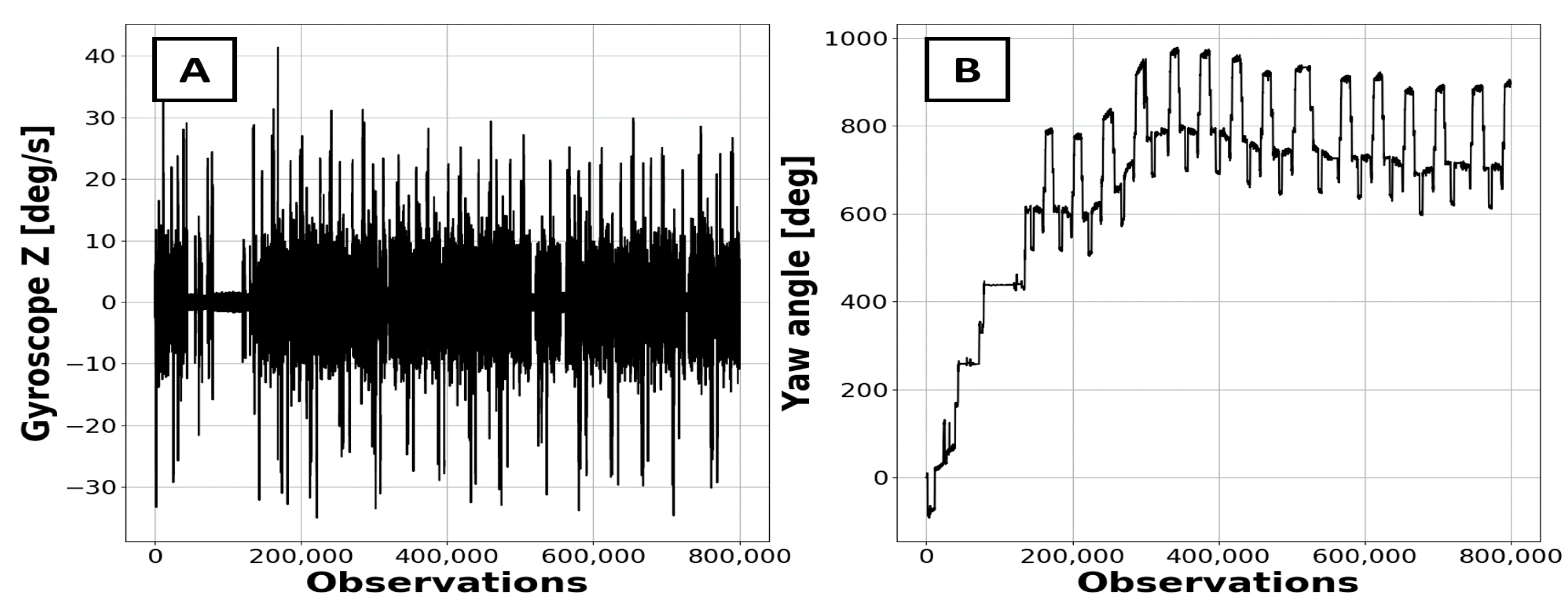
Input data for the machine turn detection algorithm was created based on gyroscope
Z-axis readings from the IMU unit. The measurement unit was embedded in a machine that was following a certain route. The sampling frequency was set to 50 Hz. A single sample used in the analysis consisted of more than 4.5-h records of sensors’ measurements from one working shift of the vehicle. During this time, a total number of 16 complete haulage cycles were recorded. Raw data from the gyroscope
Z-axis are shown in
Figure 3A. From this point, the Yaw angle (
Figure 3B) can be calculated by integration of that axis using the trapezoidal method (Equation (1)):
where
ψ is the Yaw angle at given time
τ and
is the angular speed in rotation around the
Z-axis. The Yaw angle is the most useful one from all of the Euler angles in case of turn detection. The angle describes the machine rotation around the
Z-axis, that is, its movements when viewed directly from above.
4. Proposed Models
Based on the input sample, a machine turning moments detection model was developed. Before that, however, the sample had to be manually classified, to determine the correct class labels and enable an objective evaluation of the results. The precision of such a marking was set to 1 s, which is sufficient given the relatively low speed achieved by haul trucks in underground excavations. Then, during a process of exploratory data analysis, a set of statistical indices was proposed, from which the feature vector was constructed. The next step was to balance the total number of classes appearing in the dataset. Then, using data prepared this way, several selected models were learned and the results obtained were compared on the test sample.
4.1. Preparation of the Test and Training Samples
Two types of turns have been distinguished to prepare the sample. The 70–100 degrees turns were tagged by class “1” and 40–70 degrees turns were classified as class “2.” Everything other than the previously described turn was marked as “0” (the turn did not take place). After analyzing the first results of the classification, it was decided, however, to merge classes 0 and 2 into one, as it yields significantly better results. This is because very few turns in the range of 40–70 degrees were identified in the considered sample, making this class significantly underrepresented (because most of the intersections in the mine are crossed in angle close to 90 degrees), and difficult to identify by the tested models. On the other hand, merging classes 1 and 2 resulted in a poorer fit of the tested models. Therefore, finally, only two classes were considered: 70–100 degree turns and other.
Then, the entire sample was split into a 70:30 ratio, creating the training sample used to train the selected classifiers and a test sample to validate the obtained results.
To better visualize the obtained results, by connecting the speed (obtained from the vehicle’s internal monitoring system) with the Yaw angle, the machine position in time on a plane, described by the X and Y axes can be achieved [
12]. This enables a very intuitive evaluation of the algorithm’s results and is presented later in the article. The speed variable itself is not used in the classification process.
4.2. Feature Vector
Feature vector was created by aggregating Yaw angle signal generated from the gyroscope into 1-s windows, and calculating a set of statistical indices within those windows. The initially considered indices are: mean, standard deviation, sample range, median, interquartile range, kurtosis, root mean square (RMS), skewness, and variance. Given the IMU sampling rate of 50 Hz, all of the statistical indices were calculated using 50 observations. To select the target group of indices, the distribution of their values with the considered classes was checked: “0”—no turn, “1”—90° turn, and “2”—a slight turn (as shown in
Figure 4). The total length of the obtained feature vector is 16,200.
The key statistical indices for the classification problem are those for which the most significant differences between the value for class 1 (“turn”) and the other two classes can be observed. For this purpose, data exploration was performed, and the three most visible relationships identified are presented in
Figure 5. Finally, five statistics have been selected to create the final feature vector: standard deviation, dispersion (min-max range), median, interquartile range, and kurtosis.
4.3. Selected Models
The five selected models chosen to solve the problem are logistic regression [
15], quadratic discriminant analysis (QDA) [
16], linear discriminant analysis (LDA) [
17], SVM, and the random forest model [
18].
As mentioned, it was finally decided to use the convention of dividing the sample into two classes (class “0”: no-turn and slight turns; class “1”: turns close to 90 degrees). For the two-class classification problem, the logistic regression model is often chosen as the first one checked. Logistic regression is one of the simplest machine learning tools. This method is based on a logit function defined as the logarithm of odds [
19] (Equation (2)):
The next two models (QDA and LDA) were also initially designed for the two-class classification, although their generalizations for the multi-class problem are also widely used. The LDA method finds a linear combination of features (introduced into the model) to distinguish the classes in the best way possible. This method has a very wide range of possible applications, more advanced applications being, for instance, face-recognition algorithms. LDA method assumes that observations from each of the classes have a Gaussian distribution, and covariances are identical. The QDA model is a generalization of the LDA model. It can also be used when the assumption of equal covariance is not met.
Another model considered in the article is the Support Vector Machine, which is an extension of the support vector classifier, which enables enlarging the feature space by using different kernels. This allows for non-linear boundaries between the classes. SVM models tend to perform well in a variety of different settings.
The last of the considered models is the random forest model. That method is based on the construction of multiple decision trees. Each of the trees assigns a given observation to one of the considered classes, and then the final assignment is being made based on those individual predictions. Single, deep decision trees very often overfit the training data, especially when lots of input parameters are considered. This means that the decision trees can have great accuracy when predicting samples from the training dataset (90–100%), but when given new data, the accuracy often drops to very low level, often not significantly better than a coin-flip in the case of a two-class problem. Additionally, single trees are often very non-robust, meaning that relatively small changes in the training sample can greatly impact the final estimated trees. The random forest model counteracts this phenomenon; therefore, it was chosen in this case.
All of the described models were implemented by using the sklearn library available in Python. It was established that 70% of the sample will be used to train the model and the remaining 30% will be used as a test sample.
4.4. Imbalanced Sample Problem
When training the model, the problem of an imbalanced sample was encountered. This difficulty concerns the data, where one of the classes is represented by a relatively small number of observations when compared to the second class. The case of an unbalanced sample makes the classifier training difficult because in extreme case, incorrect classification of all the observations from the minority class may result in high accuracy. A model trained on imbalanced data will quickly learn that optimizing towards the class with a higher number of occurrences by default leads to better results if the measure of accuracy is the percentage of correctly classified observations.
In our sample, the turns accounted for approx. 3.9% of all the observations (assuming that only “2” are turns; if we consider classes “1” and “2” as turns, the percentage increases to approx. 6.3%), which is shown in
Figure 6A. The problem of an unbalanced sample can be solved by various methods [
20]. In this case, two ways for balancing the sample have been considered: the undersampling (
Figure 6C) and the oversampling methods (
Figure 6B). The first of them involves removing samples from the majority class, and the second on making copies of the minority class. Both scaling methods can be used jointly; however, in this case, joining both methods did not give as good results as using them separately. An important aspect of using sampling methods is the appropriate selection of the scaling parameter. This parameter corresponds to the ratio of the number of samples in the minority class (turns) over the number of samples in the majority class (no turns) after resampling. The easiest way to select the scaling parameter is to make several tests and compare the results obtained using various scaling parameters.
5. Results
Initially, all previously described models were learned on an unbalanced and balanced sample and their results were compared. In the case of balancing, various methods and combinations of scaling were tested. All actions were described with commonly used measures assessing the accuracy of the model in class recognition. Of all the combinations, one model was selected and subjected to a final cross-validation.
5.1. Comparison of the Results of All Tested Models
To compare the model predictions to the actual data, confusion matrices and various accuracy scores were used. These were calculated using scikit-learn library built-in functions. If the results were promising, a visual test and cross-validation were performed. In the case of logistic regression, the ROC curve was also tested.
The initial models used the mentioned statistic indices (median, standard deviation, kurtosis, sample range, and interquartile range) as input parameters. Model evaluation was performed using a variety of measures mostly based on a confusion matrix [
21]. To evaluate the model accuracy (the ratio of the sum of TP (true positive) and TN (true negative) to all observations), confusion matrix, sensitivity (the ratio of TP to P (all positive)), specificity (the ratio of TN to N (all negative)), negative predictive value (the ratio of TN to the sum of TN and FN (false negative)), precision (the ratio of TP to sum of TP and FP (false positive)), and F1 score (two times the ratio of the product of sensitivity and precision to the sum of sensitivity and precision) was used. Furthermore, the macro average and weighted average (based on some previously mentioned indicators) were utilized. Results were shown in
Table 1.
It can be noticed that the LDA and the logistic regression have the best accuracy scores, but neither predict any turns, making these models invalid. This shows how the sample imbalance problem can affect the result interpretation process. The LDA model has been additionally trained and tested on the data with kurtosis and standard deviation in logarithmic scale, to improve the underlying Gaussian distribution assumption. However, this did not significantly affect the results. In the case of logistic regression, the LASSO (Least Absolute Shrinkage and Selection Operator) regularization method was also utilized (for a set of alpha parameter values 0.001, 0.01, 0.1, 1.0, 10.0) to reduce the overfitting of the model. Unfortunately, this method finally did not improve the logistic regression results on the test sample. In addition to the above-mentioned methods, the support vector machine (SVM) model with various kernel functions (linear, polynomial, and radial), and different regularization parameter and kernel coefficient were also tested. Unfortunately, when unbalanced sample is considered, the best obtained results were very similar to those of logistic regression. For this reason, in
Table 1, only the results for the SVM with linear kernel, regularization parameter equal to 1, and kernel coefficient equal to 0.5 is presented, which provided the best results. After balancing the sample, the SVM results improved, but were still inferior to those obtained by random forest. In the best case, the obtained PPV was equal to 0.04 and f1-score equal to 0.06. Among the other two models, better results were obtained for the random forest model. These results were also confirmed after rescaling the sample.
Regardless of the choice of the scaling parameter, the best results were obtained for the random forest model. The results for different methods of sample balancing for this model were shown in
Table 2. It turned out that the oversampling was better than the undersampling method in this case; therefore, only one case of the second method has been presented. In the case of the oversampling method, the results for two models that differed in the scaling parameter have been shown. In the first case, scaling to a minority was used, and in the second one oversampling was used, with a scaling parameter equal to 0.15.
5.2. The Most Accurate Prediction—A Random Forest Model
After analyzing
Table 1, it can be concluded that the best model for turn detection is the random forest, but those results were obtained on an unbalanced sample. After testing different balancing methods for all the selected classifiers, still, the best results were obtained using the random forest model. The results (shown in
Table 2) indicate that the best-matched random forest model is created based on a sample that was balanced by the oversampling method with a scaling parameter equal to 0.15. Additional tests were made (visual and cross-validation) to confirm that conclusion. The visual results of the model are presented in
Figure 7A. Many of the incorrectly verified turn’s moments (red dots) are due to the fact that the classifier has marked as a turn slightly wider or narrower sample fragment than when marked manually. The second test included a 5-fold cross-validation (
Figure 7B) and a 10-fold cross-validation (
Figure 7C). Both forms of validation confirm the good results achieved with the developed method, with an average accuracy of over 90%.
Finally, the selected random forest model was also tested on two additional samples (sample no. 2 and sample no. 3). Both samples consisted of two full working shifts of 6 h each. Sample No. 2 was recorded by the same operator as the training sample but driving a different vehicle, and sample No. 3 was recorded by a different operator and vehicle than considered in the training sample. The obtained results are presented in
Table 3. As can be seen, a random forest model can be applied to the same problem regardless of the operator driving the given type of vehicle. In the case of each tested sample, the accuracy score did not drop below 95%.
6. Conclusions
Five basic classification methods in the problem of turn identification and parametrization based on IMU readings have been compared. Their performance has been assessed on the industrial data from the KGHMs underground copper mine, registered on a haul truck operating in an underground mine, during normal operating conditions. Due to an unbalanced sample issue (fragments of the signal from the turns of the vehicle are few in training and testing sample), a scaling mechanism with a parameter equal to 0.15 was used, which vastly improved the results of considered models. Out of the tested logistic regression, linear and quadratic discriminant analysis, SVM, and random forest model, a tree-based model turned out to obtain the best results, with an accuracy score on the scaled test samples reaching over 95%. The obtained sensitivity of the model on the three test samples was 75%, 90%, and over 99%, while specificity has reached at least 97% in each case. Finally, a 5-fold and 10-fold cross-validation was performed, which also confirmed the good results of the random forest model, enabling its implementation into industrial data.
Detection of a vehicle’s turning moments requires a precise examination of those parts of the signal during which very large dynamic overloads take place, often causing damage to the structural nodes of vehicles. The presented methods can be easily extended to the similar problem of the detection of route ascents/descents, but the feature vector would have to be based on readings from a different axis of the gyroscope.
Author Contributions
Conceptualization, P.S. and B.J. methodology, J.W., B.J., and P.S.; software, J.W. and A.S.; validation, J.W., B.J., A.S., P.S. and M.D.; formal analysis, J.W., B.J. and P.S.; investigation, J.W.; resources, P.S. and P.Ś.; data curation, J.W.; writing—original draft preparation, J.W., B.J., A.S. and P.S.; writing—review and editing, J.W., B.J., A.S. and P.S.; visualization, J.W. and A.S.; supervision, P.S.; project administration, P.S. and P.Ś.; funding acquisition, P.S., P.Ś. and M.D. All authors have read and agreed to the published version of the manuscript.
Funding
This research was partially funded by the European Union’s Horizon 2020 research and innovation program, grant number 869379.
Institutional Review Board Statement
Not applicable.
Informed Consent Statement
Not applicable.
Data Availability Statement
Not applicable.
Conflicts of Interest
The authors declare no conflict of interest.
References
- Krot, P.; Sliwinski, P.; Zimroz, R.; Gomolla, N. The identification of operational cycles in the monitoring systems of underground vehicles. Measurement 2020, 151, 107111. [Google Scholar] [CrossRef]
- Gawelski, D.; Jachnik, B.; Stefaniak, P.; Skoczylas, A. Haul Truck Cycle Identification Using Support Vector Ma-chine and DBSCAN Models. In International Conference on Computational Collective Intelligence; Springer: Berlin/Heidelberg, Germany, 2020; pp. 338–350. [Google Scholar]
- Saari, J.; Odelius, J. Detecting operation regimes using unsupervised clustering with infected group labelling to im-prove machine diagnostics and prognostics. Oper. Res. Perspect. 2018, 5, 232–244. [Google Scholar]
- Michalak, A.; Śliwiński, P.; Kaniewski, T.; Wodecki, J.; Stefaniak, P.; Wyłomańska, A.; Zimroz, R. Condition Monitoring for LHD Machines Operating in Underground Mine—Analysis of Long-Term Diagnostic Data. In Proceedings of the 27th International Symposium on Mine Planning and Equipment Selection—MPES 2018; Springer: Berlin/Heidelberg, Germany, 22 February 2019; pp. 471–480. [Google Scholar]
- Skoczylas, A.; Stefaniak, P.; Anufriiev, S.; Jachnik, B. Road Quality Classification Adaptive to Vehicle Speed Based on Driving Data from Heavy Duty Mining Vehicles. In Proceedings of the International Conference on Intelligent Computing & Optimization, Hua Hin, Thailand, 30–31 December 2021; Springer: Berlin/Heidelberg, Germany, 2021; pp. 777–787. [Google Scholar]
- Meiring, G.A.M.; Myburgh, H.C. A review of intelligent driving style analysis systems and related artificial intel-ligence algorithms. Sensors 2015, 15, 30653–30682. [Google Scholar] [CrossRef] [PubMed]
- Gustafson, A.; Lipsett, M.; Schunnesson, H.; Galar, D.; Kumar, U. Development of a Markov model for production performance optimisation. Application for semi-automatic and manual LHD machines in underground mines. Int. J. Min. Reclam. Environ. 2014, 28, 342–355. [Google Scholar] [CrossRef]
- Scheding, S.; Dissanayake, G.; Nebot, E.; Durrant-Whyte, H. An experiment in autonomous navigation of an underground mining vehicle. IEEE Trans. Robot. Autom. 1999, 15, 85–95. [Google Scholar] [CrossRef] [Green Version]
- Bakambu, J.N.; Polotski, V. Autonomous system for navigation and surveying in underground mines. J. Field Robot. 2007, 24, 829–847. [Google Scholar] [CrossRef]
- Larsson, J.; Broxvall, M.; Saffiotti, A. A navigation system for automated loaders in underground mines. In Field and Service Robotics; Springer: Berlin/Heidelberg, Germany, 2006; pp. 129–140. [Google Scholar]
- Duff, E.; Roberts, J.; Corke, P. Automation of an underground mining vehicle using reactive navigation and opportunistic localization. In Proceedings of the 2003 IEEE/RSJ International Conference on Intelligent Robots and Systems (IROS 2003) (Cat. No. 03CH37453), Las Vegas, NV, USA, 27–31 October 2003; Volume 4, pp. 3775–3780. [Google Scholar]
- Skoczylas, A.; Stefaniak, P. Localization System for Wheeled Vehicles Operating in Underground Mine Based on Inertial Data and Spatial Intersection Points of Mining Excavations. In Proceedings of the Intelligent Information and Database Systems: 13th Asian Conference, ACIIDS 2021, Phuket, Thailand, 7–10 April 2021; Springer International Publishing: New York, NY, USA, 2021; Volume Proceedings 13, pp. 824–834. [Google Scholar]
- Van Ly, M.; Martin, S.; Trivedi, M.M. Driver classification and driving style recognition using inertial sensors. In Proceedings of the 2013 IEEE Intelligent Vehicles Symposium (IV), Gold Coast, Australia, 23–26 June 2013; IEEE: Piscataway, NJ, USA, 2013; pp. 1040–1045. [Google Scholar]
- Dorr, D.; Grabengiesser, D.; Gauterin, F. Online driving style recognition using fuzzy logic. In Proceedings of the 17th International IEEE Conference on Intelligent Transportation Systems (ITSC), The Hague, The Netherlands, 24–26 September 2014; IEEE: Piscataway, NJ, USA, 2014; pp. 1021–1026. [Google Scholar]
- Wright, R.E. Logistic regression. In Reading and Understanding Multivariate Statistics; Grimm, L.G., Yarnold, P.R., Eds.; American Psychological Association: Washington, DC, USA, 1995; pp. 217–244. [Google Scholar]
- Srivastava, S.; Gupta, M.R.; Frigyik, B.A. Bayesian quadratic discriminant analysis. J. Mach. Learn. Res. 2007, 8, 1277–1305. [Google Scholar]
- Li, W.-B.; Sun, L.; Zhang, D.-K. Text Classification Based on Labeled-LDA Model. Chin. J. Comput. 2009, 31, 620–627. [Google Scholar] [CrossRef]
- Ho, T.K. The random subspace method for constructing decision forests. IEEE Trans. Pattern Anal. Mach. Intell. 1998, 20, 832–844. [Google Scholar] [CrossRef] [Green Version]
- Cramer, J.S. The origins and development of the logit model. In Logit Models from Economics and other Fields; Tinbergen Institute: Amsterdam, The Netherlands, 2003; pp. 1–19. [Google Scholar]
- He, H.; Garcia, E.A. Learning from Imbalanced Data. IEEE Trans. Knowl. Data Eng. 2009, 21, 1263–1284. [Google Scholar] [CrossRef]
- Novaković, J.D.; Veljović, A.; Ilić, S.S.; Papić, Ž.; Milica, T. Evaluation of classification models in machine learning. Theory Appl. Math. Comput. Sci. 2017, 7, 39–46. [Google Scholar]
| Publisher’s Note: MDPI stays neutral with regard to jurisdictional claims in published maps and institutional affiliations. |
© 2021 by the authors. Licensee MDPI, Basel, Switzerland. This article is an open access article distributed under the terms and conditions of the Creative Commons Attribution (CC BY) license (https://creativecommons.org/licenses/by/4.0/).


 ,
, 


