Modulus of Elasticity for Grain-Supported Carbonates—Determination and Estimation for Preliminary Engineering Purposes

Featured Application

Modulus of elasticity for grain-supported carbonate rocks is successfully estimated by using simple estimation models. The methodology and models described in this paper can help engineers in the early design stages when they need a quick and easy estimate.

Abstract

The determination and estimation of elastic behaviour are essential in engineering practise, especially in quarrying, mining, construction, and all engineering professions that perform operations dealing with rock materials. Young’s modulus, or modulus of elasticity, is the most important property describing the deformability of rock material. In this paper, grain-supported carbonates from Croatia are described and their elastic modulus and significant physical and mechanical properties are determined. The analysis of the collected data was performed in the R statistical environment. Estimation models based on multiple linear regression and the regression tree model were created. The methodology of model development and evaluation in R environment is described in detail. According to the more stringent coefficients (RMSECV and adjusted R²) used to evaluate the success of the estimation, simple regression tree models were found to perform well for the preliminary estimation, while more complex models based on Bagging performed very well.

1. Introduction

The elastic behaviour of rock materials and the degree of their elasticity are essential in engineering practise for solving problems in quarrying and mining [1], construction [2], in civil engineering [3], or in tunnelling when the stress field changes due to excavation [4]. Although shear modulus, bulk modulus are used to determine the elastic behaviour of rocks [5,6,7], this paper deals with Young’s modulus, which, along with Poisson’s ratio, is the most important property in solving geomechanical problems [8,9].

The determination of the modulus of elasticity is one of the most demanding variants of testing under uniaxial load due to the use of sophisticated measurement techniques. The accuracy of the results is a major challenge for researchers and a quantitative methodology is constantly proposed to correct them [10,11]. In addition to direct determination, in certain engineering situations, it is necessary to estimate the modulus of elasticity. These estimate models can be simple or very sophisticated. The simple ones are based on diagrams and single regression equations, but sophisticated ones use platforms based on neural networks, fuzzy logic and other sophisticated algorithms that are not available to a wider range of engineering practice [12]. This shortcoming has been overcome by the authors of this paper through the use of R, which is a free software environment and as such is available to a wider range of users. R is a programming language for implementing various statistical and graphical techniques. It is extensible through many sets of functions and therefore one of the leading statistical software used for data science analysis [13]. Moreover, simple models, such as regression equations and regression trees, as well as complex models, such as the Random forest, can be created in it [14,15]. Random forest modelling is increasingly used for a variety of purposes [16], and can also be used as a variant of a regression tree to estimate the uniaxial compression strength for mudstone and wackestone carbonates [17] and sandstones [18]. When it comes to elastic modulus, simple regression equations [19,20,21,22,23,24] have been mostly used for its estimation, followed by multiple regression equations [25,26,27], neural networks [28], and other modern platforms for estimation are used with them [29,30,31].

The modelling of elastic behaviour may be based on one or more physical and mechanical rock material properties. The most common properties on which it is estimated are the Schmidt hardness and the uniaxial compressive strength [19,20,21,22,23], P-wave velocity [20,21,22], porosity [32,33]. Density and point load test index are used in combination with the above properties [25,26,27].

In previous papers [19,21], the rock material studied was determined in very general geological terms, so that often only the basic lithology was found. The influence of mineral grain on the strength and fracture behaviour of rock material has been recognised and used for numerical studies [34,35,36,37]. However, there is an obvious need for a more detailed evaluation of rock material petrological properties. In the case of carbonate rocks, these may be depositional textural features. Sedimentological investigations of carbonate rocks and determination of their physical and mechanical properties are continuously carried out in Croatia [17,34,38,39,40], but also in other places in the world where these rocks occur [41,42,43,44].

Considering the origin and composition of rocks, different varieties of carbonate sedimentary rocks are the most common in Croatia, while igneous and metamorphic rocks are less represented than sedimentary rocks [45,46]. The origin of sedimentary rocks is associated to the very thick deposits of Adriatic Carbonate Platform (AdCP) that include a major part of the entire carbonate succession of the Croatian Karst and ranges in age from the Middle Permian to the Eocene [47]. Rocks in Croatia are formed in environments with various depositional conditions; this paper is focused on grain-supported carbonates with packstone and grainstone depositional texture. Many engineering works in Croatia are associated with different carbonates, and so in this way, it is possible to determine the rock material more precisely and, based on this, to create estimation models that are specific to these textures. The aim of this work is to take a step in this direction.

The need of engineers for a quick estimate of the elastic modulus in the field was observed. Accordingly, a macroscopic petrographic analysis of different types of carbonates in terms of their depositional textures was carried out. Then, the basic physical and mechanical properties, including the elastic modulus, were determined. Based on the obtained data, the elastic modulus was also estimated using the methods (multiple linear regression, regression tree and their generalisations), which was the main objective of the work. This method proved to be useful for rapid on-site estimation of elastic modulus in engineering works.

2. Materials and Methods

The examined material came from eight locations in Croatia (Figure 1) and had a depositional texture of grain-supported packstones or grainstones. During in situ sampling, limestone and dolomite samples with different grain-support depositional textures were collected. It was also important to consider the geographic distribution of all eight sites. Dolomite samples were collected from two different sites, one from the Škrobotnik quarry in the western part of Croatia and the other from the construction notch of the road near Brušane in the central part of Croatia. Limestone samples were collected from six sites, four of which are located on the Istrian peninsula. In Korenići and Kanfanar, the material was taken from the roof deposits of the underground quarry, and in Salakovci and Trget, the material was taken from the construction excavation. In addition, limestone samples were taken from quarries in Međurače (mainland Croatia) and in the Debelo brdo exploration field (central part of Croatia).

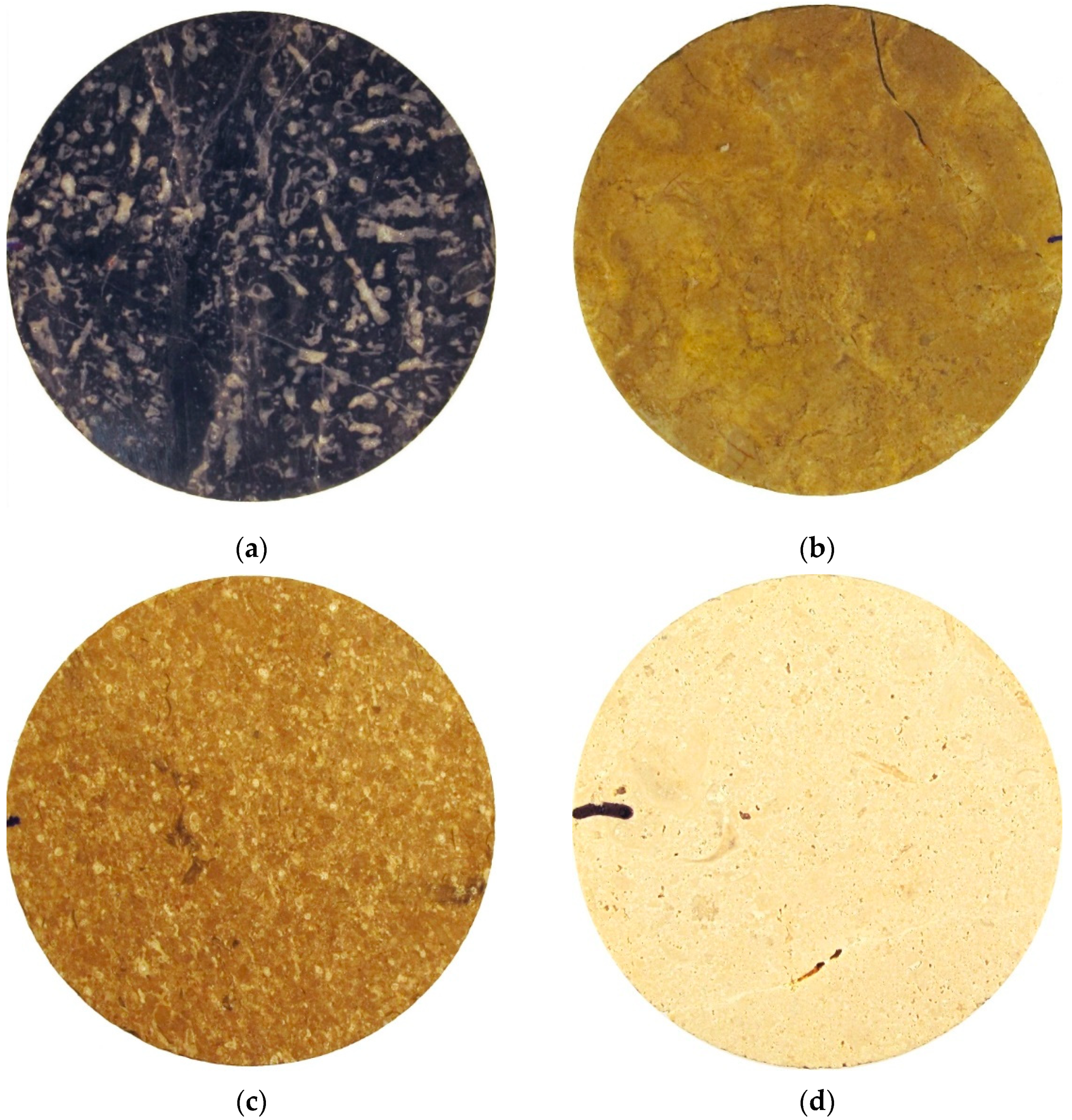
2.1. Grain-Supported Carbonates

Carbonate sedimentary rocks as petrographic group are represented by various types of limestones and dolomites. Limestones and dolomites can be classified according to their macroscopic characteristics by Dunham [48]. Dunham’s classification distinguishes and describes different carbonate rocks according to their depositional textures. Limestones are determined by the presence or absence of micrite (muddy calcareous particles < 4 µm), the ratio of grain and micrite content, and signs of organogenic skeletal bonding. Dunham’s classification distinguishes five basic types of limestones: mudstone, wackestone, packstone, grainstone and boundstone.

Packstone and grainstone (Figure 2) are both grain-supported carbonates. In such carbonates, different types of grains are mutually supporting each other while the gaps between them are filled with carbonate mud (micrite) or carbonate cement (sparite). Both packstones and grainstones have dimensions of grains lesser than 2 mm but with different content of carbonate mud (micrite). While packstone contains micrite, grainstone has less than 1% of micrite and pore spaces are dominantly filled with sparite cement (coarse crystalline calcite cement). In order to use Dunham’s classification for dolomites, it is important that the primary depositional texture was not destroyed during dolomitization, adding the prefix dolo to the name [49].

2.2. Methods for Determining Young’s Modulus and Other Properties

There are three different equivalent methods of determining the Young’s modulus of elasticity for rock material under uniaxial pressure, and it can be calculated in three different ways: as a tangent, as a secant, and as an average modulus [50]. The determination can also be made during repetitive loading and unloading cycles or under monotonic loading conditions [51]. Measurements were performed during testing under monotonic loading conditions, from which stress and strain diagrams were constructed, and the values for the modulus of elasticity were determined. The average Young’s modulus of elasticity is defined as the slope of the straight-line portion (Figure 3a) of the stress-strain curve for the particular test.

Then the average Young’s modulus was calculated according to the Formula (1).

$$E=\Delta \sigma /\Delta {\epsilon }_a$$

(1)

where E is average Young’s modulus, and Δσ is change in axial stress, and Δε_a is change in axial strain. It is emphasised that the test interval for the average modulus of elasticity is not fixed by ISRM recommendations and should be adjusted for common rock, depending on how large the linear part of the stress-strain curve is.

In this study, axial deformation was measured using a Linear Variable Differential Transformer (LVDT) based displacement transducer (Figure 3b). It is designed to provide the average readings of three LVDTs that measure deformations in the axial direction. The instrument is attached to the specimen by means of tightening screws located on the rings around the specimen. Despite being robust, it measures with an accuracy of 2% and a precision of 0.2% over the entire measurement field, which is ±2.54 mm. The entire testing process, from load application to conditioning and acquisition of stress and strain data, was carried out by implementing the virtual instrument described in paper [52] to determine the uniaxial compressive strength and deformability of rock specimens.

Other properties were also determined according to ISRM recommendations [50]. These are common and well-known methods in rock mechanics that are widely used in geoengineering, so the details of each test are not presented here; only important details are pointed out. In this case, the uniaxial compressive strength (σ_c) was determined according to the peak stress required for failure of the specimen. The stress load was 0.75 MPa per second and was performed using an ELE ADR 2000 laboratory press.

Density and porosity were determined by saturation and calliper techniques, since the samples could be prepared as regular geometric shapes and did not swell on contact with water. Therefore, it was not particularly difficult to determine the total volume, and this was done by measuring the dimensions of regular samples with a calliper. Saturation of the samples was carried out with an apparatus capable of immersing the samples in water at a pressure of less than 800 Pa for one hour. A laboratory balance with a reading capacity of 0.01 g was used to determine the mass of the sample.

The point load test index was measured using the Digital Point Load Test Apparatus 77-0115. It has a load capacity of 55 kN, which was sufficient to break specimens in the form of a 54 mm diameter disk. An axial type test was performed.

Schmidt rebound hardness was determined using a Proceq SilverSchmidt L-type digital Schmidt hammer, which has an impact energy of 0.735 Nm, suitable for rock testing. The lower impact energy ensures that the specimens are not damaged for further testing.

P-wave velocity was measured using the device Cns Farnell Pundit plus, which is one of the high-frequency ultrasound devices that operate at a frequency of 1 MHz. It allows easy measurement of velocity on core-shaped samples, which were later used to determine the modulus of elasticity.

2.3. Use of R Statistical Environment for Estimating Youngs Moduli

Data analysis was performed in the R statistical environment. R is a free software environment used in the academic community for modelling and graphics. In this paper, version 4.1.0 on 64-bit Windows 10 operating system was used. In addition, some extra packages were used: leaps for displaying all linear models according to R², tree for the random tree analysis, and randomForest for bagging and the random forest model.

Linear regression is a very simple and straightforward approach for predicting a response variable Y based on a predictor X. It is assumed that there is a linear relationship between Y and X which is described by (2)

$$Y={\beta }_0+{\beta }_{1}X,$$

(2)

where β₀ and β₁ are constants.

As a linear function is determined by precisely two different points and a dataset is always bigger, the sign “=” in the last equation is changed to “≈”. In other words, for each point, there is an error. There are many points (usually all of them) that the linear function does not pass through. We say that the response variable Y is approximately modelled by the predictor variable X.

This idea can be easily generalised for more than one predictor. A multiple linear regression model can be stated as follows. It is assumed that there are p predictors X₁, X₂, …, X_p and a response variable Y. The model is given by the Formula (3)

$$Y={\beta }_0+{\beta }_1{X}_1+{\beta }_2{X}_2+\dots +{\beta }_p{X}_p+ϵ$$

(3)

where β₀, β₁, …, β_p are regression coefficients and $ϵ$ is a random error term with zero mean. The coefficient β₀ is also known as the intercept term. The interpretation of the coefficients is as follows. If X_i increase for one unit, holding all other predictors fixed, the regression coefficient β_i equals the average change of Y. In practice, the coefficients are unknown and estimated using the least squares method [14]. In the case of one predictor (k = 1), the data are organised in a set of points (x_i, y_i) where x_i is a measurement of X and y_i is a measurement of Y that corresponds to x_i. The least squares method gives “the best” line that fits the data—so that y_i ≈ β₀ + β₁ x_i, for i = 1, …, n. In the case of two predictors (k = 2), the method gives “the best” plane that fits the data. In the case of more than two predictors, there is a lack of intuition and imagination, but the model is still correct and interpretable in the described way.

After the appropriate model is fitted, the goodness of model fit is required. There are a few measures of goodness of model fit which can be useful for model selection. The quantity which is often used as a measure of the quality of the model fit is the coefficient of determination, denoted by R² and given by (4)

$$R^2=\left(TSS-RSS\right)/TSS=1-RSS/TSS$$

(4)

$$RSS={\displaystyle \sum }_{i=1}^n{\left(y_i-{\widehat{y}}_i\right)}^2$$

(5)

$$TSS={\displaystyle \sum }_{i=1}^n{\left(y_i-\overline{y}\right)}^2$$

(6)

where RSS is the residual sum of squares calculated according to Formula (5), TSS is the total sum of squares calculated according to Formula (6), ${\widehat{y}}_i$ is the predicted value for y_i using x_i and a statistical method, and $\overline{y}$ is the overall sample mean.

Total variance in the response variable (TSS) can be divided into the variance explained by the fitted model (TSS-RSS) and the variance that is left unexplained (RSS). The R² statistic takes the form of the proportion of the variability in the response variable that is explained by the model. If R² takes the value close to 1, that indicates that a large amount of variability in the response variable has been explained by the fitted model. However, it is clear that R² will increase when more variables are added to the model. If adding some new predictor to the model leads to just a tiny increase in R², then it can be dropped from the model [14]. Adding such predictors to the model also leads to overfitting. Therefore, it is useful to have more measures of goodness of model fit.

One such measure is an improved version of R², called adjusted R², which adjusts thevpreviously described R² by taking into account the size of the dataset and number of parameters in the model. It is given by (7).

$$adj R^2=1-\frac{RSS/\left(n-d-1\right)}{TSS/\left(n-1\right)}$$

(7)

where n is a number of observations and d number of included parameters.

RSS always decreases as the number of predictors in the model increases, but RSS/(n − d − 1) may increase or decrease, due to the presence of d in the denominator. Once all of the correct variables have been included in the model, adding additional “needless” variables will lead to a very small decrease in RSS.

There are some measures of model performance that are more computationally exhaustive. One of them is a root mean square error of cross-validation (RMSECV). It is based on a cross-validation. The cross-validation procedure splits the dataset into a training set and test set finitely many times (the number of splitting is set in advance). The leave-one-out cross-validation puts a single observation in the test set, while other observations make up the training set. A statistical method is repeated n times on n − 1 observations, and each time a prediction is made for one particular observation that is left out. In every repeat, the squared error is calculated. The estimate for the overall mean squared error is the average of these n errors, denoted by CV_(n) (9) [14]. RMSECV is given by (8).

$$RMSECV=\sqrt{C{V}_{\left(n\right)}}$$

(8)

$$C{V}_{\left(n\right)}=\frac{1}{n} {\displaystyle \sum }_{i=1}^n{\left(y_i-{\widehat{y}}_i\right)}^2$$

(9)

where n is the number of observations, y_i is the observed ith value and ${\widehat{y}}_i$ is the predicted value for y_i using x_i and a statistical method fitted on the remaining n − 1 observations. The main advantage of this model accuracy measure is its unbiasedness.

After choosing a few representative linear models according to these two measures of model accuracy, it is good to check to see which one of them is the best. Assume that there are two models: the one with k predictors complete model (10) and the reduced model (11) with one predictor less than the complete model.

$$Y={\beta }_0+{\beta }_1{X}_1+\dots +{\beta }_{k-1}{X}_{k-1}+{\beta }_k{X}_k+ϵ$$

(10)

$$Y={\beta }_0+{\beta }_1{X}_1+\dots +{\beta }_{k-1}{X}_{k-1}+ϵ$$

(11)

Models of that kind are called nested models. It is of interest whether the distinguished predictor, when it is added to the model, contributes to the quality of the model. Hypotheses are set as follows (12) and (13):

$$H_0: {\beta }_k=0$$

(12)

$$H_1: {\beta }_k\ne 0$$

(13)

For this purpose, the F-test for nested models is performed. The test statistic is given by (14).

$$F=\frac{\frac{RS{S}_R-RS{S}_C}{p_C-p_R}}{\frac{RS{S}_C}{n-p_C}},$$

(14)

where RSS_C and RSS_R are the residual sum of squares for the complete and reduced model, respectively. Further, $p_C$ and $p_R$ are the numbers of predictors in the complete and reduced model and n is the length of the dataset. If the null hypothesis is true, the test statistic has an F distribution with ($n-p_R$) and ($n-p_C$) degrees of freedom.

For performing this statistical test in R the “anova” function is used. The level of significance is set to 5%. The same F statistic can be used for testing the hypothesis that more than one coefficient β_i equals 0.

The regression tree method divides the data into smaller groups that are more homogenous with respect to the response variable. The process starts with the whole dataset and searches every distinct value of every predictor to find the predictor X_k and split value s that partitions the data into two groups S₁ = {X|X_k < s} and S₂ = {X|X_k ≥ s} such that the overall sums of squares are minimised (15)

$${\displaystyle \sum }_{i \in S_1}{\left(y_i-{\overline{y}}_1\right)}^2+{\displaystyle \sum }_{i \in S_2}{\left(y_i-{\overline{y}}_2\right)}^2$$

(15)

where ${\overline{y}}_1$ and ${\overline{y}}_2$ are the averages of the training set outcomes within groups S₁ and S₂, respectively [15].

The process continues within each group in the same manner until the number of observations in the splits falls below some threshold (usually, the threshold is 5). That kind of splitting is a type of greedy algorithm known as recursive binary splitting. At the end of the recursive process, the data are divided into N disjoint subsets S₁, S₂, …, S_N called terminal nodes or leaves. Each of the terminal nodes is presented by the average of the response variable of observations settled in that node.

After the tree has been grown, it can be very large and complex and is likely to overfit the training set. The tree is then pruned back to a smaller tree (a subtree of the full tree constructed by the above procedure).

The structure of the regression tree constructed by the described procedure highly depends on the training set. Bagging, short for bootstrap aggregation, is a general approach that uses the combination of bootstrapping and regression trees to produce a suitable prediction model. First, different training datasets are generated from the original data. On every bootstrapped training dataset, a regression tree is structured. For the given values of predictors, M predictions of the response variable $\left({\widehat{y}}_1, {\widehat{y}}_2, \dots , {\widehat{y}}_M\right)$ are obtained and then averaged to give the bagged model’s prediction (16).

$${\widehat{y}}_{bag}=\frac{1}{M}{\displaystyle \sum }_{i=1}^M{\widehat{y}}_i$$

(16)

The described approach usually improves predictive performance for unstable models, like regression tree models. In the case of a large number of bootstrap samples, bagging is a computationally exhaustive method. Another disadvantage is that trees from different bootstrap samples may have similar structures to each other (especially at the top of the trees) due to a relationship between one strong predictor and response. This feature is known as tree correlation, and it prevents bagging from optimally reducing the variance of the predicted values $\left({\widehat{y}}_1, {\widehat{y}}_2, \dots , {\widehat{y}}_M\right)$ [15]. Adding randomness to the construction procedure can reduce the correlation among predictors. Random forest is such a method which at each split randomly selects m predictors from the whole set of p predictors. The number m is known as the random forests’ tuning parameter, and the recommended choice is m = p/3 or √(p) (in this paper, p = 6, so m = 2).

Since there is a collection of bagged trees, results of the random forest method and bagging are less interpretable than the results of a single tree model. However, measures of predictor importance can be constructed by combining measures of importance from the individual models across the set of M constructed trees. The total amount that the RSS is decreased due to splits over a given predictor is averaged over all M trees. A large value is interpreted as an important predictor.

3. Results

3.1. Petrographic Characteristics and Physical-Mechanical Properties

To determine their petrographic characteristics and to relate them to physical and mechanical properties macroscopic observation was done. The textural characteristics were determined on 33 in situ carbonate samples. Among them on seven dolomites and on 26 limestone samples (Figure 4 and Figure 5). The samples were classified into packstone and grainstone groups according to the depositional texture.

All dolomite samples (four from Brušane—Figure 4a and three from Škrobotnik—Figure 4b) were determined as dolograinstones with visibly preserved primary depositional textures and grains with grain-support. Brušane samples were represented by grey to black laminated dolomites with partially visible fossil grains while Škrobotnik samples are dark yellowish laminated dolomites.

Unlike dolomites, limestone samples were determined as both grainstones and packstones. Two out of seven grainstone samples are from the Korenići and five are from Salakovci location. Yellowish to brown homogenous limestones from Salakovci (Figure 4c) are determined as foraminiferal grainstones with dimensions of grains from 1 to maximum 5 mm. Light yellow limestones with fossil fragments from Korenići (Figure 4d) show visible anisotropy (lamination) and have high primary porosity with pores up to 3 mm.

There is a total of 19 limestone samples determined as packstones: two of them from Međurače, three from Debelo brdo, and seven from each Trget and Kanfanar location. Međurače limestone (Figure 5a) is of red to brown colour with randomly oriented white wide fissures subsequently filled with calcite cement. Debelo brdo limestones (Figure 5b) are dark in colour probably due to organic matter content. In addition, samples show visible lamination and stylolite type fissures. Yellowish samples from Trget (Figure 5c) have homogeneously distributed fossil fragments with dimensions from 0,1 to 3 mm. Kanfanar samples (Figure 5d) are yellowish with clearly visible fossils (oncoids) up to 3 mm in micritic base. Small fissures represented by stylolitic seams filled with calcite cement are also visible.

In addition to petrographic analysis, laboratory samples were prepared from 33 field samples for a total of 231 physical-mechanical properties tests. General descriptive statistics of all test results are presented in

Table 1. General descriptive statistics of grain-supported carb onates test results.

General Statistics	$\mathit{\rho }$	n	Is(50)	SRH	vp	σc	E
min	2376	0.14	0.5	38.2	4944	51.44	38.38
max	2823	11.25	6.8	72.5	6378	181.36	93.26
average	2634.64	3.22	4.30	59.05	5710.12	126.81	57.11
standard deviation	122.10	3.01	1.43	8.98	389.80	32.45	12.99
Coefficient of variation (%)	4.63	93.48	33.26	15.21	6.83	25.59	22.75

$\rho$—density (kg/m³); n—porosity (%); I_s(50)—point load test index (MPa); v_p—P wave velocity (m/s); SRH—Schmidt rebound hardness; σ_c—uniaxial compressive strength (MPa); E—Young’s modulus of elasticity (GPa).

.

The wide range of all studied properties (from minimum to maximum) shows that the collected rocks with packstone and grainstone texture have quite different physical and mechanical properties. The minimum value of uniaxial strength is 51.44 MPa and the maximum value is 181.36 MPa. According to the Marinos and Hoek [53], it means that the rock material belongs to the category of strong (from 50 to 100 MPa) and very strong rock (from 100 to 250 MPa). The tests showed that the values of the modulus of elasticity ranged from 38.38 to 93.26 GPa with a standard deviation of 12.99 GPa. It is worth noting that according to the coefficient of variation, the largest scatter of data is for porosity with an average value of 3.22% and the smallest for density (average 2634.64 kg/m³) and P-velocity (average 5710.12 m/s).

Ideally, rock material density should be related solely based on density of its mineral composition, but measured density (analysed by saturation technique) also reflects isolated pore spaces. Consequently, the difference in measured densities is primarily caused by a slightly higher density of dolomite in comparison to calcite but is also influenced by rock material porosity (Figure 6).

These are the main reasons for obvious clustering of density data according to recognised texture types. Despite of some differences in physical properties of various types of grain-supported carbonate rocks, the same diagram does not indicate significant difference in elastic modulus for particular texture types. For that reason, the elastic modulus is studied for the whole group of grain-supported carbonate rock materials.

The relationships between the predictors via the correlation coefficient were also studied, and the result is shown graphically in Figure 7.

Logically, the relationship between porosity and density is a negative strong relationship. That is the reason why those two independent variables do not appear both in the same models that are proposed later. The values of the correlation coefficient between other predictors are small so, evidently, there is no significant relationship.

3.2. Models for Estimating Modulus of Elasticity

In this paper, multiple linear regression models for all subsets of six predictors are built (p = 6). There are 63 subsets in total and the best three models according to RMSECV are given by:

$$E=-112.194+0.026\rho -2.000I_{S\left(50\right)}+0.017v_p+0.123{\sigma }_c$$

(17)

$$E=-135.388+0.035\rho +0.016v_p+0.093{\sigma }_c$$

(18)

$$E=-61.014-2.806I_{S\left(50\right)}+0.02v_p+0.137{\sigma }_c$$

(19)

where E is the modulus of elasticity (GPa), $\rho$ is density (kg/m³), I_S(50) is the point load strength index (MPa), v_p is the P-wave velocity (m/s), σ_c uniaxial compressive strength (MPa). The constructed regression tree is shown in Figure 8.

Variables used in the tree construction (Figure 8) are: the P-wave velocity (v_p), the point load strength index (I_s(50)), Schmidt rebound hardness (SRH), and uniaxial compressive strength (σ_c). They stand as the most important predictors for the prediction of modulus of elasticity. In function “prune.tree” the parameter “best” equals the number of terminal nodes. If there is no tree of a certain size, the next largest is constructed. Since the tree in Figure 8 has five leaves, the pruned tree could have three or four leaves. Of specific interest may be the one with four leaves (and three most important predictors) shown in Figure 9.

As previously mentioned, the analysis with random forest is obtained by setting parameter m to 2, while in bagging, that parameter is set to 6 (parameter “mtry” in function “randomForest”). Figure 10 displays the importance of predictors in the random forest model. In the sense of the amount of reduced RSS, the most important predictor is the P-wave velocity (v_p) and the least important is uniaxial compressive strength (σ_c).

4. Discussion

The identification and differentiation of carbonate rock material texture is very important because it indicates many factors which have great impact on its physical and mechanical properties as: grain content and sizes, matrix composition and quality, and porosity [34,39]. Therefore, it is necessary to focus research on individual categories. Given that the most engineering work (mining, quarrying, tunnelling) is performed in different varieties of carbonate rocks this research was based on grain-supported limestones and dolomites. According to the macroscopic petrographic characteristics, it is evident that the packstone samples slightly differ from the grainstone ones. Grainstone samples (

Table 2. Number of samples according to lithology and depositional texture.

Location	Lithology	Depositional Texture	Number of In Situ Samples
Škrobotnik, Brušane	dolomite	dolograinstone	7
Korenići, Salakovci	limestone	grainstone	7
Međurače, Debelo brdo, Trget, Kanfanar	limestone	packstone	19

) generally have visible anisotropy in the shape of lamination. Only Salakovci samples are homogenous. Fossil fragments are bound together with cement while fossil fragment in packstones are bound together with micrite. Packstone samples (Table 2) are mostly homogenous (only Debelo brdo has visible lamination). Regardless of the slightly visible petrographic differences according to the gained data of physical and mechanical properties, packstones behave similarly to grainstones and are therefore taken together for modelling. Generally, determined grain-supported carbonates are considered to be compact and to have good properties with low porosity. Most of the samples are without secondary defects while only few samples show visible minor defects (subsequently filled fissures with calcite cement as Međurače).

Average Young’s modulus of elasticity for the grain-supported textures of packstone and grainstone was studied. It should be noted that in previous papers [8,9] a more appropriate tangent modulus was evaluated for modelling the estimate. However, in the same papers, a very high similarity between the average and tangent modulus is also noted. The similarity is the reason why the authors in this paper nevertheless opt for a more determined average modulus. Of course, one should always pay attention and emphasise how the Young’s modulus is determined, since, for example, the values of the secant type of modulus can be very different.

Data analysis and estimation modelling were performed in the R statistical environment. The advantage of the R statistical environment is that it is free and available. Nevertheless, great strides have been made in the R-studio variant, which is more acceptable for use in mining, construction, and related professions.

Multiple linear regression, regression tree, and its generalisations are considered. In the case of multiple linear regression, 63 models were constructed as all possible combinations of six predictors. They are compared using two measures of accuracy of the model: adjusted R² and RMSECV (

Table 3. RMSECV, adjusted R² values and their ranking numbers for multiple linear regression models.

Linear Model	RMSECV Rank (Value)	Adjusted R2 Rank (Value)
(17)	1. (10.0025)	4. (0.5129)
(18)	2. (10.0313)	7. (0.4890)
(19)	3. (10.0798)	8. (0.4837)

). It is obtained using a leave-one-out cross-validation. The best result according to RMSECV is achieved by the models (17) and (18).

The model with all predictors included takes the 24th place according to the RMSECV and the 2nd place according to the adjusted R².

Model (17) and (18) are compared using F-test. Model (17) is considered as the complete and model (18) as the reduced model. The p-value is 0.1309 which is greater than 0.05 so the null hypothesis is rejected. The point load strength index as a predictor variable significantly contributes to the quality of prediction of the modulus of elasticity.

If models (17) and (19) are compared in the same manner, the p-value equals 0.1091 which leads us to the same conclusion for the density as a predictor variable.

On the other hand, the regression tree model (

Table 4. Measures of accuracy of the three models.

Models	RMSECV	R2	Adjusted R2
Regression tree (Figure 8)	10.2387	0.7624	0.7285
Pruned tree (Figure 9)	10.0712	0.7424	0.7157
Bagging (m = 6)	9.8033	0.8934	0.8687
Random Forest (m = 2)	10.1133	0.8736	0.8652

RMSECV—root mean square error of cross-validation; R²—coefficient of determination.

) has a larger adjusted R² than every linear model. The models based on regression trees give significantly better results according to R² and adjusted R². Except for bagging, they give slightly worse results due to the value of RMSECV.

The size of the R² models in this paper was compared with those in other papers [30,31,43]. One obstacle to the comparison is that the same success coefficients were not used, so the comparison can only be made using the size R² that all models had. This is most evident when comparing the R² model which was created using artificial neural networks which have a black box in their structure and therefore cannot explain their outputs, and it has undesirable negative properties such as complexity in its multilayer structure, possibility of overlearning [31]. Taking this into consideration, it can only be argued that the models developed in this paper have lower R² than the neural network models [43].

It is noticeable that the most successful model Bagging in this paper has a very similar value R² (0.8934) to the model created earlier, whose coefficient of determination is 0.908 [31], and it was created using the Least Square Support Vector Machine method (LS-SVM). This is an advanced version that is superior to the artificial neural networks method in terms of predictive performance, generality, and robustness. This is consistent with the research of [29] who investigated the advantages and disadvantages of fuzzy inference systems, artificial neural networks and LS -SVM methods and found that the performance of the LS -SVM model was the best among the other methods. However, the small difference in R² between the models in this paper and [31] shows the similarity of the success of both models and does not imply that the Bagging model is less useful or less accurate. More so, if the emphasis is on simplicity and great attention is paid to avoiding overfitting, then it is quite justified to use the models of the authors of this paper, as they have used other very rigorous measures (RMSECV and adjusted R²) to evaluate model performance.

Of course, it is important to point out that the results of this study do not replace laboratory tests on the elastic properties of rocks, which still need to be carried out. The analysis in this paper shows that for a simpler prediction of elastic rock properties using pruned tree, it is sufficient to know the data of three parameters (P-wave velocity, uniaxial compressive strength and the point load strength index). To reliably predict the elastic rock properties, the remaining four parameters are also used for modelling. Therefore, the application of this method in engineering practice depends on the amount of available data. Actual application of this method in engineering practice is possible in the preliminary stages of work to improve property estimation when direct determination of elastic modulus would be uneconomical. For example, when it is desired to preliminarily investigate the possibility of exploitation of natural stone for a material that has been tested in some construction project. This is only an example, and it depends on the engineering professionals to what extent they will use the estimates and to what extent they will perform the determination of the modulus of elasticity.

5. Conclusions

Based on the study of the grain-supported carbonates from Croatia with depositional textures of packstone and grainstone, as well as on the models created for estimation, it can be concluded:

• Petrographic characteristics of rocks have proven to be extremely important since they directly affect the physical and mechanical properties and modulus of elasticity. According to the obtained results, the packstone and grainstone carbonates from Croatia show similar properties and can be mutually combined when estimating the modulus of elasticity of carbonates. Still, it is important to point out that presented results consider low porosity carbonates without or with minor secondary defects. Other types of carbonate rock materials may have considerably different properties, therefore better results, it is suggested that each group of carbonates is considered and estimated separately.
• It is useful in engineering terms to create simple estimation models based on multiple regression and regression trees, and in this sense, the R statistical environment has proven to be a viable and accessible platform.
• Regression tree models can be used to easily estimate the modulus of elasticity for carbonates with packstone and grainstone textures with input parameters of P-velocity, uniaxial compressive strength, and point load test index.
• The bagging tree model showed the best evaluation results. Its performance parameters are 0.8934 for R² and 0.8687 for adjusted R². This model can be used with input parameters listed in the previous point, as well as density, porosity and Schmidt rebound hardness.

References

1. Lanciano, C.; Salvini, R. Monitoring of Strain and Temperature in an Open Pit Using Brillouin Distributed Optical Fiber Sensors. Sensors 2020, 20, 1924. [Google Scholar] [CrossRef] [PubMed] [Green Version]
2. Moayedi, H.; Kalantar, B.; Abdullahi, M.M.; Rashid, A.S.A.; Nazir, R.; Nguyen, H. Determination of Young Elasticity Modulus in Bored Piles Through the Global Strain Extensometer Sensors and Real-Time Monitoring Data. Appl. Sci. 2019, 9, 3060. [Google Scholar] [CrossRef] [Green Version]
3. Zhussupbekov, A.; Alibekova, N.; Akhazhanov, S.; Sarsembayeva, A. Development of a Unified Geotechnical Database and Data Processing on the Example of Nur-Sultan City. Appl. Sci. 2021, 11, 306. [Google Scholar] [CrossRef]
4. Mohyla, M.; Vojtasik, K.; Hrubesova, E.; Stolarik, M.; Nedoma, J.; Pinka, M. Approach for Optimisation of Tunnel Lining Design. Appl. Sci. 2020, 10, 6705. [Google Scholar] [CrossRef]
5. Rybacki, E.; Reinicke, A.; Meier, T.; Makasi, M.; Dresen, G. What controls the mechanical properties of shale rocks?—Part I: Strength and Young’s modulus. J. Pet. Sci. Eng. 2015, 135, 702–722. [Google Scholar] [CrossRef]
6. Wetzel, M.; Kempka, T.; Kühn, M. Predicting macroscopic elastic rock properties requires detailed information on microstructure. Energy Procedia 2017, 125, 561–570. [Google Scholar] [CrossRef]
7. Wetzel, M.; Kempka, T.; Kühn, M. Diagenetic Trends of Synthetic Reservoir Sandstone Properties Assessed by Digital Rock Physics. Minerals 2021, 11, 151. [Google Scholar] [CrossRef]
8. Małkowski, P.; Ostrowski, Ł. The methodology for the Young modulus derivation for rocks and its value. Proceedia. Eng. 2017, 191, 134–141. [Google Scholar] [CrossRef]
9. Malkowski, P.; Ostrowski, L.; Brodny, J. Analysis of Young’s modulus for Carboniferous sedimentary rocks and its relationship with uniaxial compressive strength using different methods of modulus determination. J. Sustain. Min. 2018, 17, 145–157. [Google Scholar] [CrossRef]
10. Kuhinek, D.; Zoric, I.; Hrzenjak, P. Measurement uncertainty in testing of uniaxial compressive strength and deformability of rock samples. Meas. Sci. Rev. 2011, 11, 112–117. [Google Scholar] [CrossRef] [Green Version]
11. Abdelaziz, A.; Grasselli, G. How believable are published laboratory data? A deeper look into system-compliance and elastic modulus. J. Rock Mech. Geotech. Eng. 2021, 13, 487–499. [Google Scholar] [CrossRef]
12. Briševac, Z.; Hrženjak, P.; Buljan, R. Models for estimating uniaxial compressive strength and elastic modulus. Građevinar 2016, 68, 19–28. [Google Scholar] [CrossRef] [Green Version]
13. The R Project for Statistical Computing. Available online: https://www.r-project.org/about.html (accessed on 7 June 2021).
14. James, G.; Witten, D.; Hastie, T.; Tibshirani, R. An Introduction to Statistical Learning with Applications in R; Springer: New York, NY, USA, 2017; pp. 59–126. [Google Scholar]
15. Johnson, K.; Kuhn, M. Applied Predictive Modelling; Springer: New York, NY, USA, 2016; pp. 173–203. [Google Scholar]
16. Zhang, H.; Zhou, J.; Jahed Armaghani, D.; Tahir, M.M.; Pham, B.T.; Huynh, V.V. A Combination of Feature Selection and Random Forest Techniques to Solve a Problem Related to Blast-Induced Ground Vibration. Appl. Sci. 2020, 10, 869. [Google Scholar] [CrossRef] [Green Version]
17. Briševac, Z.; Špoljarić, D.; Gulam, V. Estimation of uniaxial compressive strength based on regression tree models. Min. Geol. Pet. Eng. Bull. 2014, 29, 39–47. [Google Scholar]
18. Liang, M.; Mohamad, E.T.; Faradonbeh, R.S.; Armaghani, D.J.; Ghoraba, S. Rock strength assessment based on regression tree technique. Eng. Comput. 2016, 32, 343–354. [Google Scholar] [CrossRef]
19. Dinçer, I.; Acar, A.; Çobanoğlu, I.; Cobanoglu, I.; Uras, Y. Correlation between Schmidt hardness, uniaxial compressive strength and Young’s modulus for andesites, basalts and tuffs. Bull. Eng. Geol. Environ. 2004, 63, 141–148. [Google Scholar] [CrossRef]
20. Yasar, E.; Erdogarg, Y. Correlating sound velocity with the density, compressive strength and Young’s modulus of carbonate rocks. Int. J. Rock Mech. Min. Sci. 2004, 41, 871–875. [Google Scholar] [CrossRef]
21. Kahraman, S.; Yeken, T. Determination of physical properties of carbonate rocks from P-wave velocity. Bull. Eng. Geol. Environ. 2008, 67, 277–281. [Google Scholar] [CrossRef]
22. Moradian, Z.A.; Behnia, M. Predicting the uniaxial compressive strength and static young’s modulus of intact sedimentary rocks using the ultrasonic test. Int. J. Geomech. ASCE 2009, 9, 14–19. [Google Scholar] [CrossRef]
23. Yagiz, S. Predicting uniaxial compressive strength, modulus of elasticity and index properties of rocks using the Schmidt hammer. Bull. Eng. Geol. Environ. 2009, 68, 55–63. [Google Scholar] [CrossRef]
24. Azimian, A.; Ajalloeian, R. Empirical correlation of physical and mechanical properties of marly rocks with P wave velocity. Arab. J. Geosci. 2015, 8, 2069–2079. [Google Scholar] [CrossRef]
25. Gokceoglu, C.; Zorlu, K. A fuzzy model to predict the uniaxial compressive strength and the modulus of elasticity of a problematic rock. Eng. Appl. Artif. Intell. 2004, 17, 61–72. [Google Scholar] [CrossRef]
26. Yilmaz, I.; Yuksek, G. Prediction of the strength and elasticity modulus of gypsum using multiple regression, ANN, and ANFIS models. Int. J. Rock Mech. Min. Sci. 2008, 46, 803–810. [Google Scholar] [CrossRef]
27. Heidari, M.; Khanlari, G.R.; Momeni, A.A. Prediction of elastic modulus of intact rocks using artificial neural networks and nonlinear regression methods. Aust. J. Basic Appl. Sci. 2010, 4, 5869–5879. [Google Scholar]
28. Ocak, I.; Seker, S.E. Estimation of Elastic Modulus of Intact Rocks by Artificial Neural Network. Rock Mech. Rock Eng. 2012, 45, 1047–1054. [Google Scholar] [CrossRef]
29. Ceryan, N.; Can, N.K. Prediction of the uniaxial compressive strength of rocks materials. In Handbook of Research on Trends and Digital Advances in Engineering Geology; Ceryan, N., Ed.; Igi Global: Hershey, PA, USA, 2018; pp. 31–96. [Google Scholar]
30. Aboutaleb, S.; Behnia, M.; Bagherpour, R.; Bluekian, B. Using non-destructive tests for estimating uniaxial compressive strength and static Young’s modulus of carbonate rocks via some modeling techniques. Bull. Eng. Geol. Environ. 2018, 77, 1717–1728. [Google Scholar] [CrossRef]
31. Acar, M.C.; Kaya, B. Models to estimate the elastic modulus of weak rocks based on least square support vector machine. Arab. J. Geosci. 2020, 13, 590. [Google Scholar] [CrossRef]
32. Leite, M.H.; Ferland, F. Determination of Unconfined Compressive Strength and Young’s Modulus of Porous Materials by Indentation Tests. Eng. Geol. 2001, 59, 267–280. [Google Scholar] [CrossRef]
33. Lashkaripour, G.R. Predicting mechanical properties of mudroek from index parameters. Bull. Eng. Geol. Environ. 2002, 61, 73–77. [Google Scholar] [CrossRef]
34. Pollak, D.; Gulam, V.; Bostjančić, I. A visual determination method for uniaxial compressive strength estimation based on Croatian carbonate rock materials. Eng. Geol. 2017, 231, 68–80. [Google Scholar] [CrossRef]
35. Han, Z.; Zhang, L.; Zhou, J. Numerical Investigation of Mineral Grain Shape Effects on Strength and Fracture Behaviors of Rock Material. Appl. Sci. 2019, 9, 2855. [Google Scholar] [CrossRef] [Green Version]
36. Lakirouhani, A.; Asemi, F.; Zohdi, A.; Medzvieckas, J.; Kliukas, R. Physical parameters, tensile and compressive strength of dolomite rock samples: Influence of grain size. J. Civ. Eng. Manag. 2020, 26, 789–799. [Google Scholar] [CrossRef]
37. Park, K.; Kim, K.; Lee, K.; Kim, D. Analysis of Effects of Rock Physical Properties Changes from Freeze-Thaw Weathering in Ny-Ålesund Region: Part 1—Experimental Study. Appl. Sci. 2020, 10, 1707. [Google Scholar] [CrossRef] [Green Version]
38. Briševac, Z.; Hrženjak, P.; Cotman, I. Estimate of uniaxial compressive strength and Young’s modulus of the elasticity of natural stone giallo d’Istria. Procedia Eng. 2017, 191, 434–441. [Google Scholar] [CrossRef]
39. Pollak, D. Dependence of the Engeneerig-Geologycal Quality of the Carbonate Rocks abot Their Sedimentological and Petrological Charachteristics (Adriatic Motorway—Section “Tunnel Sveti Rok—Maslenica”). Master’s Thesis, University of Zagreb, Faculty of Mining, Geology and Petroleum Engineering, Zagreb, Croatia, 2002. [Google Scholar]
40. Maričić, A.; Starčević, K.; Barudžija, U. Physical and mechanical properties of dolomites related to sedimentary and diagenetic features—Case study of the Upper Triassic dolomites from Medvednica and Samobor Mts., NW Croatia. Min. Geol. Pet. Eng. Bull. 2018, 33, 33–44. [Google Scholar] [CrossRef] [Green Version]
41. Palchik, V. On the ratios between elastic modulus and uniaxial compressive strength of heterogeneous carbonate rocks. Rock Mech. Rock Eng. 2011, 44, 121–128. [Google Scholar] [CrossRef]
42. Barudžija, U.; Maričić, A.; Brčić, V. Influence of Lithofacies and Diagenetic Processes on the Physical and Mechanical Properties of Carbonate Rocks—Case Study from Sinawin-Sha’wa Area, Libya. Min. Geol. Pet. Eng. Bull. 2015, 30, 19–36. [Google Scholar] [CrossRef]
43. Madhubabu, N.; Singh, P.K.; Kainthola, A.; Mahanta, B.; Tripathy, A.; Singh, T.N. Prediction of compressive strength and elastic modulus of carbonate rocks. Measurement 2016, 88, 202–213. [Google Scholar] [CrossRef]
44. Palchik, V. Simple stress-strain model of very strong limestones and dolomites for engineering practice. Geomech. Geophys. Geo-energy Geo-Resour. 2019, 5, 345–356. [Google Scholar] [CrossRef]
45. Crnković, B.; Jovičić, D. Dimension stone deposits in Croatia. Min. Geol. Pet. Eng. Bull. 1993, 5, 136–163. [Google Scholar]
46. Fio Firi, K.; Maričić, A. Usage of the Natural Stones in the City of Zagreb (Croatia) and Its Geotouristical Aspect. Geoheritage 2020, 12, 62. [Google Scholar] [CrossRef]
47. Vlahović, I.; Tišljar, J.; Velić, I.; Matičec, D. Evolution of the Adriatic Carbonate Platform: Palaeogeography, main events and depositional dynamics. Palaeogeogr. Palaeoclimatol. Palaeoecol. 2005, 220, 333–360. [Google Scholar] [CrossRef]
48. Dunham, R.J. Classification of Carbonate Rocks According to Theirdepositional Texture. Classification of Carbonate Rocks—A Symposium; Ham, W.E., Ed.; AAPG Memoir: Tulsa, OK, USA, 1962; Volume 1, pp. 108–121. [Google Scholar]
49. Tucker, M.E.; Wright, V.P. Carbonate Sedimentology; Blackwell Scientific Publication: London, UK, 1990; pp. 365–400. [Google Scholar] [CrossRef]
50. ISRM Turkish National Group. The Blue Book: “The Complete ISRM Suggested Methods for Rock Characterization, Testing and Monitoring: 1974–2006”; Ulusay, R., Hudson, J.A., Eds.; ISRM Turkish National Group: Ankara, Turkey, 2007; 628p. [Google Scholar]
51. Vaneghi, R.G.; Thoeni, K.; Dyskin, A.V.; Sharifzadeh, M.; Sarmadivaleh, M. Strength and Damage Response of Sandstone and Granodiorite under Different Loading Conditions of Multistage Uniaxial Cyclic Compression. Int. J. Geomech. 2020, 20, 04020159. [Google Scholar] [CrossRef]
52. Kuhinek, D.; Zorić, I.; Hrženjak, P.P. Development of Virtual Instrument for Uniaxial Compression Testing of Rock Samples. Meas. Sci. Rev. 2011, 11, 99–103. [Google Scholar] [CrossRef] [Green Version]
53. Marinos, P.; Hoek, E. Estimating the geotechnical properties of heterogeneous rock masses such as flysch. Bull. Eng. Geol. Environ. 2001, 60, 85–92. [Google Scholar] [CrossRef]
Figure 1. Location map showing in situ sampling points.
Applsci 11 06148 g001
Figure 2. Depositional texture of packstone and grainstone types, after Dunham (1962).
Applsci 11 06148 g002
Figure 3. Determination of the average modulus of elasticity: (a) stress-strain curve; (b) LVDT based displacement transducer.
Applsci 11 06148 g003
Figure 4. Grainstone depositional textures from different locations: (a) dolomite from Brušane; (b) dolomite from Škrobotnik; (c) limestone from Salakovci; (d) limestone from Korenići.
Applsci 11 06148 g004
Figure 5. Packstone depositional texture in limestones from different locations: (a) Međurače; (b) Debelo brdo; (c) Trget; (d) Kanfanar.
Applsci 11 06148 g005aApplsci 11 06148 g005b
Figure 6. Young’s modules in relation to density and by carbonate type.
Applsci 11 06148 g006
Figure 7. Correlation between physical and mechanical characteristics, which were later used as input variables in modelling.
Applsci 11 06148 g007
Figure 8. Regression tree model (five leaves).
Applsci 11 06148 g008
Figure 9. Pruned tree for estimation of the modulus of elasticity (four leaves).
Applsci 11 06148 g009
Figure 10. Importance of variables in the random forest model due to the amount of reduced RSS.
Applsci 11 06148 g010