1. Introduction
The eyes can be considered a mirror of the human body, allowing for non-invasive diagnosis of numerous illnesses [
1]. In particular, the retina can be used as a useful indicator of many diseases. As a person grows older, several diseases leave significant indicative signs in the retina.
According to the fact sheet of the World Health Organization (WHO), blindness and vision impairment affect about
billion people around the world. One billion of them have a chance to prevent the decrease in vision if they are recognized and diagnosed at an earlier stage [
2].
Diabetic retinopathy (DR) and glaucoma, which are the focus of the present work, are regarded as the most important causes of blindness, mainly due to the progress in life prospects and permissive lifestyles [
3]. DR is a complication of diabetes that inevitably leads to the terminal state of vision loss. Glaucoma is a chronic ocular disease caused by increased fluid pressure in the optic nerve and ends up also harming peripheral vision [
4]. Globally, it is estimated that at least 6.9 million people have glaucoma and
million have DR [
5].
The International Diabetic Federation estimates that, worldwide, one in every ten people suffers from diabetes [
6], and that those persons have a significant chance to suffer from DR and glaucoma impairments. Moreover, it is estimated that the number of people who suffer from glaucoma is expected to reach
million by 2040 [
7].
DR and glaucoma are irreversible diseases, so detecting them at an early stage is critical to avoid further deterioration in the retina. On the other hand, some countries, especially in the developing world, have a severe shortage of oculist doctors [
8], requiring computer-aided diagnosis, such as the one proposed in the present work.
Luckily, images of the retina can help in diagnosing several retinal diseases, including DR and glaucoma [
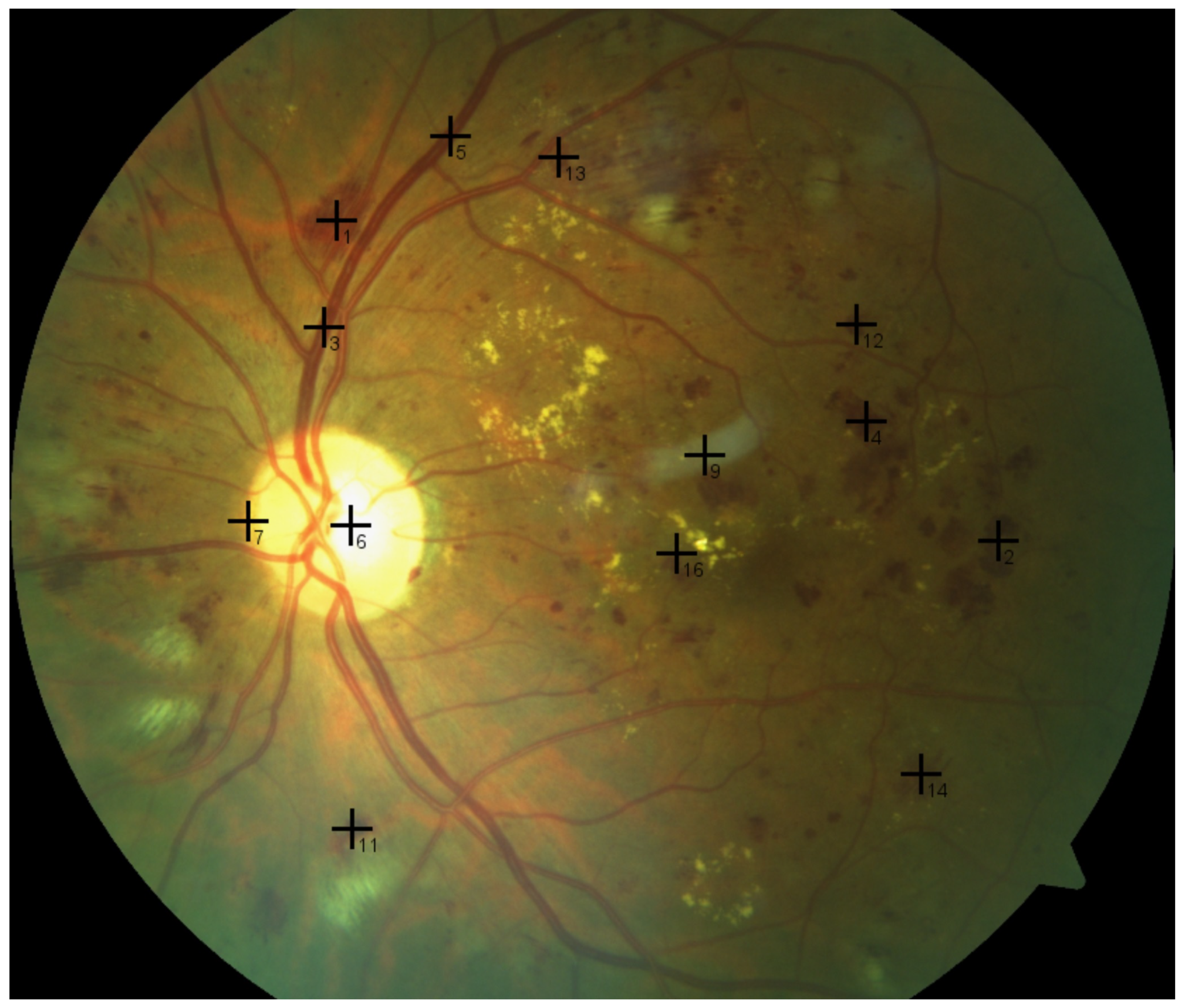
9]. This process is usually carried out and interpreted manually, which is laborious and prone to error due to minute image details, as shown in
Figure 1. Consequently, if this process is automated, it would help ophthalmologists with a supportive tool that makes both diagnosis and decision making faster, easier, less expensive, and more accurate. To this end, computer vision and imaging techniques, such as those in the present work, can be leveraged.
For ophthalmic fundus imaging analysis, well-known modalities, such as 2D fundus images and 3D optical coherence tomography (OCT), can be employed [
10]. In this study, the 2D fundus image modality is adopted due to its low cost and the simplicity in computation compared with 3D OCT modality images [
11]. To this end, we use three publicly available datasets of retinal fundus images. It should be noted, however, that disease diagnosis via pathological structures of fundus images poses numerous challenges, such as:
- 1.
Finding relevant datasets for each disease is laborious;
- 2.
Labeling (annotating) the dataset usually requires ophthalmology experts, and can be problematic due to such considerations as privacy, safety, or ethics. The only alternative is to use publicly available images, as is done in the present work;
- 3.
Subtle and tiny variations between intensity values of retinal objects, as shown in
Figure 1, can cause errors;
- 4.
The curvature of the retina, in addition to photographic capturing conditions, can often cause illumination spots in retinal fundus images, negatively affecting their quality.
- 5.
Retinal diseases share common characteristics in the fundus images, giving rise to confusion.
This article tackles the above challenges, culminating in an accurate retinal diagnostic and prognostic system that discriminates among DR, glaucoma, and normal (free of diseases) cases using a retinal fundus image. To this end, the RGB image is first transformed into its elementary components: red (R), green (G), and blue (B) channels. Then, three groups of distinct features are composed for the image. The first-order statistics (FOS) group contains 4 features per channel, giving rise to 12 features for the 3 channels. The higher-order statistics (HOS) group contains 14 features per channel per displacement, giving rise to 112 features for the 3 channels and 8 displacements. The histogram of oriented gradient (HOG) group contains 81 features. The three groups thus collectively contain 429 features that can discern between the three classes we consider. However, to make the processing more efficient, a genetic algorithm (GA)-based scheme is leveraged to select the most relevant and informative of these features, successfully reducing them to 105.
To evaluate the feature selection process and the proposed system’s performance in general, we use four machine learning (ML) classifiers: decision tree (DT), naive Bayes (NB),
k-nearest neighbor (
kNN), and linear discriminant analysis (LDA). Based on our experimentation with other classifiers, such as support vector machine (SVM), random forest (RF), and Adaboost, and based on our previous work [
12] with artificial neural networks (ANNs) in the same image processing context, the four chosen classifiers provide higher accuracy, easier setup, fewer training images, and less training and/or testing time. It is possible, however, that a classifier that we did not experiment with performs better using the proposed features than the chosen four.
The article is organized as follows.
Section 2 surveys previous work on retinal CAD systems, especially feature extraction and image classification.
Section 3 describes the retinal fundus datasets used in our experiments and the methodology adopted in feature extraction and selection.
Section 4 provides the results of the experimental work and discusses their implications and the gained insights, with the discussions of those results presented in
Section 5. Finally, concluding remarks are given in
Section 6.
2. Related Work
A sizable amount of research exists for disease diagnosis through retinal fundus images. The research can be categorized in six directions. The first direction is the binary computer-aided diagnosis (CAD) system that is based on retinal blood vessel segmentation [
13]. The second direction is binary CAD systems dedicated to identifying age-related macular degeneration (AMD) disease [
9]. The third direction is binary retinal CAD systems mainly devoted to segmenting the optic disc (OD) region [
3]. The fourth direction includes multi-class CAD systems devoted to grading the progress levels of only DR [
14], or only glaucoma [
15]. The fifth direction includes binary CAD systems used to classify more than one retinal disease together, such as DR and/or glaucoma and/or AMD. These diseases are identified, however, one at a time, as either existing or not using binary classification [
16]. The sixth direction includes multi-class CAD systems applied to classify several retinal diseases together and evaluates them as a multi-classification problem [
17]. This direction is the most relevant to the present work, and is therefore reviewed in detail next, with
Table 1 summarizing its highlights.
An automatic lesion detection system is proposed by [
23] for early detection of DR-related lesions. A bag-of-visual-words (BoVW) algorithm is employed to discriminate among different DR lesions using a maximum margin classifier. Despite the robustness of the system, its only purpose is to identify the different types of DR signs rather than grading the DR severity.
Ganesan et al. [
18] suggest a binary CAD system for DR detection by experimenting on two datasets of images. The RGB fundus image is transformed into a gray-level image. Out of a total of 840 extracted features, only 670 meaningful features are used. This system leverages a support vector machine (SVM), probabilistic neural network (PNN), and PNN improved by a genetic algorithm (PPN-GA). In spite of the effectiveness of the system, its binary operation is a limitation. Moreover, the system is designed to find whether the pathology is DR positive, without determining the severity grade of the disease.
Mookiah et al. [
19] present a CAD system based on nonlinear feature extraction to distinguish between normal and AMD images. The feature vector is encoded and provided to a SVM classifier. The system is tested on three datasets, one private and two public, the public being automated retinal image analysis (ARIA) and structured analysis of the retina (STARE). The system exhibits an accuracy of
,
, and
for the ARIA, private, and STARE datasets, respectively. Aside from the fact that the system is dedicated to only AMD diagnosis, it is only valid when the retinal image resolution is uniform.
Qaisar et al. suggest an automatic retinal system to recognize the five severity levels of DR: normal, mild NDPR, moderate NPDR, severe NPDR, and PDR [
24]. This system was developed using deep visual features (DVFs) and was tested on fundus images from three public datasets and one private.
All the systems mentioned above are applied to diagnose only a single disease in the image dataset. Next, we will review work that is directed at multi-disease diagnosis DR, AMD, and glaucoma.
A system dedicated to identifying DR, AMD, and glaucoma is presented by [
20]. The system is based on decomposing the fundus image into
intrinsic mode functions (IMFs) to detect the pixels’ morphological variations. The system leverages an SVM classifier to differentiate between pathological symptoms pertaining to DR, AMD, and glaucoma and normal images. The system performance achieved
,
, and
for accuracy, sensitivity, and specificity, respectively. Although this system considers three diseases, the final decision output is a binary classification (normal or abnormal).
Koh et al. [
16] present a two-class CAD system dedicated to identifying DR, AMD, glaucoma from fundus images. In total, 404 normal and 1082 abnormal fundus images were experimented on. The system achieved
,
, and
for overall accuracy, overall sensitivity, and overall specificity, respectively, using 15 features. Although the system uses four classes of images (AMD, DR, glaucoma, and normal), the system only predicts binary classification (normal or abnormal) for each disease. Since there are
more abnormal fundus images than normal ones, this imbalance makes the system’s final decision more biased towards the abnormal class.
In a subsequent work, Koh et al. [
22] present another CAD system to identify three retinal diseases, AMD, DR, and glaucoma. The bag-of-visual-words approach and Gaussian mixture model (GMM) were carried out on the training dataset to build the vocabulary. Random forest (RF) was employed as a classification model. However, aside from the fact that the system was tested on a private dataset of images, a requirement for reproducibility, the final results are somewhat disappointing. The reason why the results are not impressive could be because the system depends on the extracted vocabulary from image patterns, not from the image pixels themselves. In addition, the final results are provided on an aggregate basis, i.e., for all three classes of cases, DR, glaucoma and normal.
ANN in general and deep learning in particular have also been used heavily for ophthalmic diagnosis using retinal fundus images. An overview of the applications of deep learning of this topic is presented in [
25], where the authors describe image datasets that can be used for deep learning purposes, and applications of deep learning for segmentation of the optic disc, optic cup, and blood vessels as well as detection of lesions.
A retinal CAD system based on deep residual NN classifiers using small labeled images is presented in [
17]. The system employs three tasks related to eye disease diagnosis. The first is identifying five broad categories, DR, AMD, glaucoma, melanoma, and normal images. The second is predicting one of the 320 fine-grained disease sub-categories (grades). The third is creating a textual explanation for the diagnosis. Experimenting on a dataset of 7212 labeled and 35,854 unlabeled images from 3502 patients, the system achieved an overall accuracy of
,
, and
for the three tasks, respectively, which are low compared to the results of the present work.
A medical image analysis based on deep mining for screening DR is proposed by Quellec et al. [
26], aiming to detect the four different DR lesion types in fundus images. Specifically, a deep convolutional NN with 26 different layers acts to automatically detect pathological features.
A combined convolutional NN and recurrent NN were developed for heightened glaucoma detection [
27]. The CNN/RNN combined model attained an average
F score of
in identifying glaucoma. This system suffers, however, from low accuracy if the number of training images is not large enough.
A retinal CAD system based on a deep learning technique is presented by Zhao et al. [
28]. A transfer deep learning architecture depends on a residual NN, including feature attention and channel re-calibration to extract features from the retinal fundus image. RGB Kaggle fundus images were used after pre-processing steps to mitigate noise effects of the background. This system resulted in
for the area under the curve (AUC) of the receiver operating characteristic (ROC) and
for overall accuracy. This system is highly robust, but the computational cost is relatively high.
In [
29], a deep learning system is proposed to study its efficacy in diagnosing and grading glaucomatous optic neuropathy (GON) through retinal fundus images. The network comprises twenty-two layers, of which eleven are inception-v3 architecture modules. Out of 70,000, 48,116 fundus images were selected to be annotated by ophthalmology doctors (twenty-seven doctors) for labeling as GON images or not GON images. A minibatch gradient descent of a size of thirty-two was used for training using an Adam optimizer, with an initial learning rate of
. The final results achieved for the system were 0.929, 0.956, and 0.920 for accuracy, sensitivity, and specificity [
29].
A multi-layer perceptron (MLP) NN and hand-crafted features are presented by Tamim et al. [
12], using retinal fundus images to diagnose DR by searching pixel by pixel in the retinal image for biomarkers of DR lesions. The system uses 24 hand-crafted features and a 3-layer NN. A post-processing technique depending on mathematical morphological operators is used to optimize the blood vessel segmentation procedure. A selected vector of features is proposed in this study. In comparison, three publicly available datasets are used. The experimental results, visually and quantitatively, indicate the robustness of the suggested methods. The proposed method gave 0.960, 0.754, and 0.984 for the DRIVE dataset, 0.963, 0.780, and 0.982 for the STARE dataset, and 0.957, 0.758, and 0.984 for the CHASSE_DB1 dataset, for accuracy, sensitivity, and specificity, respectively. Despite the robustness of this method, it is dedicated to only one unique ocular disease,
DR.
The use of NNs and deep learning is still the focus of much research in the area of retinal image analysis. For example, a technique based on a gray wolf optimized NN is presented by Jerith and Kumar [
30] for early recognition of glaucoma using retinal images. They first converted the original color images into gray-level, then the artifacts due to noise were suppressed using an adaptive median filter. The extracted features comprised gray-level co-occurrence matrix (GLCM) features, speedup robust features, histogram of oriented gradient (HOG) features, and global features that were encoded for gray wolf optimization.
In [
31], Maqsood et al. studied hemorrhage detection based on a 3D CNN deep learning framework and feature fusion for evaluating retinal abnormality in diabetic patients. A pre-trained modified CNN model was employed to extract features to form a feature vector. The feature vector was fused by convolutional sparse image decomposition, and later the best features were selected by multi-logic regression controlled entropy variance techniques. They achieved 0.9771 for the average accuracy.
Li et al. [
29] proposed a deep learning system to detect glaucomatous optic neuropathy from retinal fundus images. Their NN comprised 22 layers, with 11 inception-v3 architecture modules. Out of 70,000 images, 48,116 fundus images were selected for annotation by ophthalmologists as GON or not GON. The final results achieved for the system were 0.929, 0.956, and 0.920 for accuracy, sensitivity, and specificity, respectively.
In [
32], Ramasamy et al. studied detection of DR using a fusion of textural and ridgelet features of retinal images and a sequential minimal optimization classifier. The ocular features were extracted and fused based on co-occurrence, run-length features, and ridgelet transform coefficients. The method was tested using sequential minimal optimization through retinal ocular images. The sensitivity, specificity, and accuracy obtained were 0.9887, 0.9524, and 0.9705 for the DIAREKDB1 dataset, and 0.909, 0.91, and 0.910 for the Kaggle dataset, respectively.
The problem with deep learning, however, is that it acts mostly as a black box, with plenty of stacked layers, providing little knowledge about local features at the image level. Furthermore, its training requires a huge number of images, which may not be readily available. For example, the work by Quellec et al. [
26] depends on 90,000 images from Kaggle and 110,000 images from e-ophtha, in addition to 89 DiaretDB1 datasets. Another problem with deep learning is that it is remarkably time-consuming, primarily during training but also during testing. All these drawbacks are mitigated in the approach followed in the present work which depends mainly on hand-crafted features and conventional ML models.
3. Materials and Methods
Despite the huge body of work in the field of eye CAD systems, there is a gap in handling and classifying more than one retinal disease at once (direction six above), in particular distinguishing between cases of DR, glaucoma, and normal conditions in fundus images. This could be due to the scarcity of publicly available fundus images, especially ones with both glaucoma and DR. It could also be due to the fine and subtle differences between the intensity values of different pathological patterns (pixels) in the images, as shown in
Figure 1. The present work is intended to bridge this gap.
It should be noted that both normal and DR fundus images are macula centered, so FOS and HOS features are applied for characterizing the pathological pattern of DR. On the other hand, glaucoma fundus images are OD centered [
22]. Thus, HOG features are used to identify the pathological pattern for glaucoma.
To obtain an accurate retinal CAD system, this study employs three groups of hybrid features and a modified genetic algorithm (GA)-based scheme, resulting in the following contributions:
- 1.
A fully automated system that is easy to use.
- 2.
The classification model is developed using a balanced number of retinal fundus images in each class, ensuring robustness.
- 3.
The center pixel of the OD in Dataset_2 is identified using three expert ophthalmologists, expediting the cropping of the OD for further processing and reaching the quality of the High-Resolution Fundus (HRF) dataset.
- 4.
The model utilizes all the three channels (red, green, and blue) of images, capturing all potential information in the fundus image.
- 5.
Three different groups of feature extractors are used to carefully obtain an optimal number of 429 features, ensuring both accuracy and efficiency.
- 6.
A modified genetic algorithm is used as a feature selector to select the most relevant features among all the 429 extracted features.
- 7.
Classifying more than two cases, DR, glaucoma and normal conditions, from the fundus image opens the door to generalization where any number of cases can be identified.
- 8.
In-depth analysis plus a fair comparison with the nearest state-of-the-art systems.
The proposed system is based on texture features extracted from the region of interest (ROI) of the retinal fundus images. FOS features and HOS features are extracted from all three RGB channels to characterize DR disease, while HOG features are extracted from the optical disc (OD) region in gray-level images. The system encompasses four main stages: color transformation, feature extraction, feature selection, and classification, as shown in
Figure 2.
The RGB color model is commonly used in CAD systems because it is based on the three primary colors embedded in most computerized input and output devices, unlike the HSV model which is closer to how humans perceive color. As such, it lends itself readily to digital image processing in general and digital retinal image research in particular. Even the few attempts that initially use HSV, such as the attempt by Zhou et al. [
33], to provide some lamination and contrast enhancement for poor-quality images eventually revert back to RGB for further processing.
In the beginning, the RGB image is processed in two steps. The first step is to transform the RGB image into its essential R, G, and B channels. The second step is to identify and crop the OD region using the given center pixel location and the OD’s diameter. The cropped OD region is converted into gray-scale.
Next, three different feature sets, FOS, HOS, and HOG, are then used for constructing three different sets of features that can distinguish between the pathological and normal patterns for each disease. The first set, FOS, consists of four features: mean, variance, skewness, and kurtosis while HOS features are 14 textural features: angular second moment (ASM), contrasts, correlation, sum of squares (variance), inverse difference moment (homogeneity), sum average, sum entropy, sum variance, entropy, difference variance, difference entropy, information measure of correlation 1, information measure of correlation 2, and auto-correlation.
The third set, HOG, comprises 81 features. Both FOS and HOS extractors are used to gather the statistical texture information for the entire retinal R, G, and B image, whereas HOG is employed to detect intensity changes in the gray-scale cropped OD region image. At the end of feature extraction, a feature vector with 429 distinct features is constructed.
In the next stage, a feature selection technique based on modified genetic algorithms is applied to reduce the feature space, which positively affects the final system performance.
In the last stage, four classifiers, decision tree (DT), k-nearest neighbor (kNN), naive Bayes (NB), and linear discriminant analysis (LDA) are used to make the diagnosis decision.
3.1. Data Acquisition
The first dataset in our work, High-Resolution Fundus (HRF) [
34], comprises 45 RGB images of three different classes, DR, glaucoma, and normal conditions, with 15 images per class. The HRF dataset is provided with ma annotation by three expert ophthalmologists, specifying the OD center pixel location and the diameter of the OD. The second dataset, Dataset_2, consists of 288 RGB fundus images assembled from datasets. First, 192 images are from the Kaggle DR dataset [
35] (96 images for DR class and 96 for the normal class). The remaining 96 images for glaucoma are collected from the BinRashed Eyes Glaucoma dataset [
36]. Thus, the classes of Dataset_2 are balanced in that each class contains 96 images. Since Dataset_2 was acquired from two different sources, unlike HRF, it needs to be manually annotated to locate the OD center pixels. For this task, we made use of the expertise of three skilled ophthalmologists from King Fahd Central Hospital (KFCH), Saudi Arabia, who ably specified the center pixel and the diameter of the OD. The two datasets used in the present work thus have three classes, DR, glaucoma, and normal (free of disease). The DR and normal images are macula centered, while the glaucoma images are OD centered.
Table 2 provides general information related to the two image datasets.
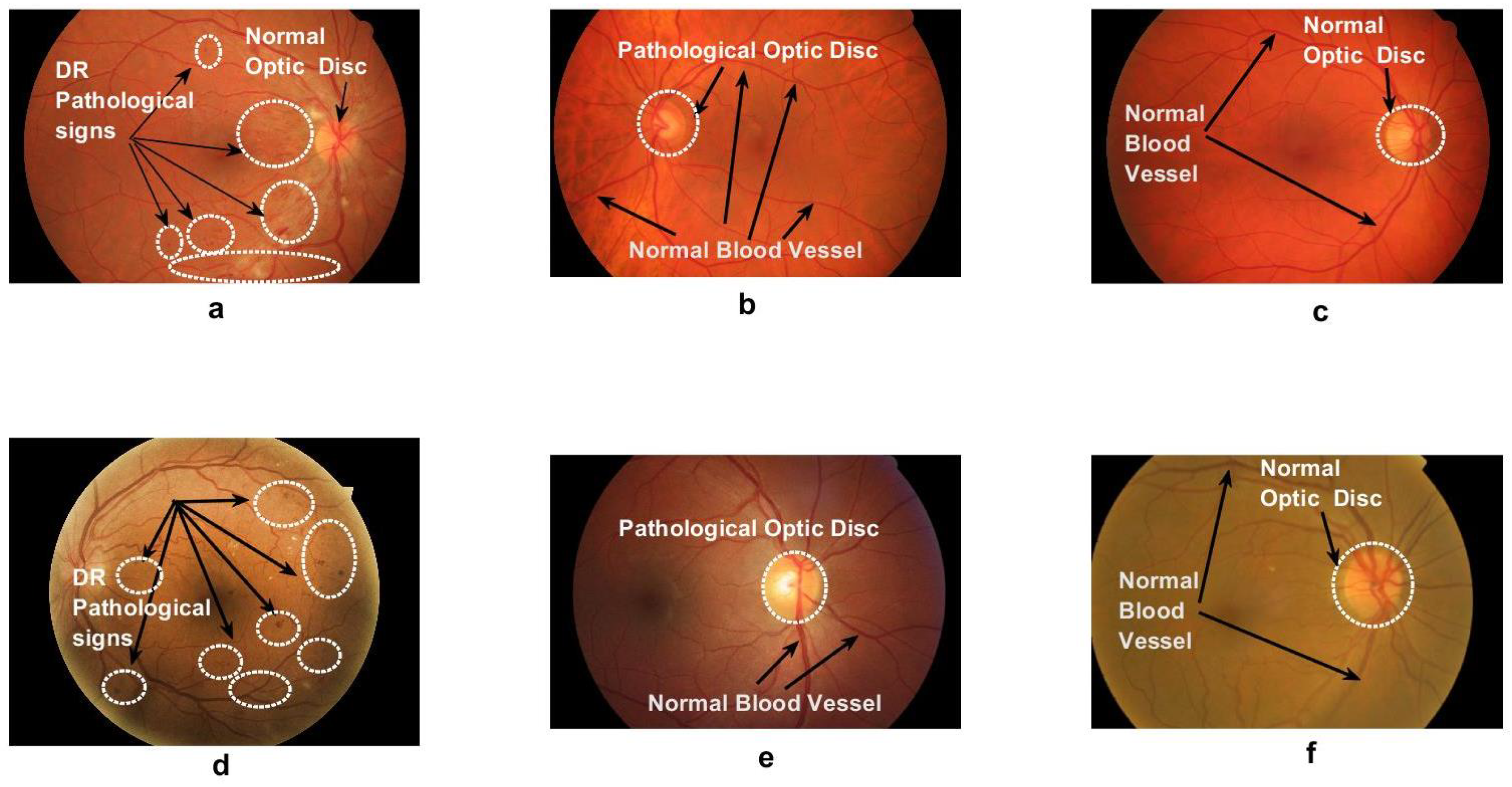
Figure 3 shows the different pathological patterns for DR and glaucoma compared to the normal cases.
3.2. Feature Selection
Feature selection reduces the amount of linearly dependent features to extract useful independent information for a given problem. Unlike prior work on diagnosing diseases through retinal fundus images, where the green channel of the RGB image is commonly used, in the present work, the three channels, red (R), green (G), and blue (B) are used to capture all the information available in the image. In addition, we make use of the gray-level version of the image because the textural features are mainly based on the spatial repetition of any two neighbor pixels in that version.
With the above in mind, three different feature sets are used to represent the retinal fundus image: FOS, HOS, and HOG. This is in sharp contrast to the less suitable method where only the green channel is used.
3.2.1. FOS Features
FOS texture features are the most straightforward and most commonly used to represent the image textural characteristics [
37]. They are intensity based and mainly computed from a histogram of gray-level values of the image. They include mean, variance, skewness, and kurtosis which specify some of the image’s textural characteristics and are obtained from the distribution of intensity values and individual pixel values in an image, as follows.
Let an image I, of size pixels, where H and W are the height and width, respectively, of I in pixels. Then,
- 1.
The mean,
, gives information concerning the central tendency of the pixel intensities in the image. If
,
,
is a given pixel and
is the intensity of that pixel, then the mean of
I is given by
- 2.
The variance
, where
is the standard deviation, determines how the intensities of pixels are scattered around the mean intensity
and is given by
- 3.
The skewness
gives knowledge regarding the symmetry of the gray-level values around the mean. A given distribution of data is symmetric if it looks the same to the left and right side of the mean, as in the normal distribution; otherwise, it is skewed left or right, and the skewness is given by
- 4.
The kurtosis,
, concerns the peakedness of the pixel intensity distribution in the image’s histogram. It is a measure of the extreme values in the tail of the distribution, with a large kurtosis indicating that the tail peakedness exceeds that of the normal distribution. Data distributions with low kurtosis exhibit tail data that are generally less extreme than the normal distribution tails. The kurtosis is given by
Though simple to compute, FOS features ignore the spatial relationship between pixels and their surrounding neighbors. So, this group is not sufficient to quantify or discriminate between changes in retinal images [
38].
3.2.2. HOS Features
The second set of features, HOS, contains textural features based on the gray-level co-occurrence matrix (GLCM) obtained from a 2D gray image [
39]. The GLCM helps extract relevant textural features from an image by tracking the spatial distribution of pixels inside the region of interest (ROI) of the gray image. It is prevalent in medical image analysis and pattern recognition [
40].
Consider a retinal 2D gray image,
, with
L gray levels and of size
pixels. We could characterize the textural information in terms of the frequent occurrence of the intensity of a reference pixel value,
i, to its adjacent neighbor pixel value,
j, with a predefined distance
d and orientation
. To quantify this image, the concept behind Haralick feature extraction [
39] is to map it from the range
, as a bit depth, into the range
, which holds the solicited number
of the gray level. The map quantization function,
, is defined as
Then, the quantized image,
, is given by
The non-normalized GLCM matrix is denoted by
, and its elements are obtained from the quantized image,
, through counting the number of times every pair of adjacent gray-level pixels occurs as a neighbor in the image
, or in an arbitrary area thereof. The neighborhood relation between pixels in terms of displacement between any two adjacent pixels can be defined by a displacement vector,
, in the
x and
y directions, with
representing the displacement in the
x and
y directions in terms of pixels with distance
d. In the present work,
. Each entry,
, in
is given by
The entry
tallies how many times gray values of the two nearby pixels occur in
, with
.
According to the pioneering work of Haralick, eight displacement vectors can be used on 2D fundus retinal images to establish the direction within two adjacent pixels, as shown in
Figure 4.
The eight displacement vectors described above are used in this work to conduct all possible relationships for the adjacent pixels in the eight directions in
. Therefore, in this work, there are eight GLCMs for each
. Once
is constructed based on a particular direction vector, then it is normalized, yielding the normalized GLCM:
where
is the probability mass function for the gray level of adjacent pixels in
. So, the normalized matrix,
, contains information about the retinal image pixels that have similar gray-level values, which is used later to compute the textural features for each of the eight displacement vectors per gray image.
The 14 textural features of an image are obtained from the
matrix, noting that
is the number of gray levels in the quantized image [
41].
- 1.
The angular second moment (ASM),
, feature is a measure of the consistency of textural information in an image. A consistent image is characterized by very few dominant gray level transitions between its pixels, and its related
matrix contains fewer entries of large magnitude. The more homogeneity in the image, the larger the value of ASM, with the range of this value being
. The
feature is given by
- 2.
The contrast feature,
, is a measure of the status of the local variations in the intensity values between pixels of an image. The higher the local variation value, the larger the contrast. Contrast also represents a measure of intensity variation between a reference pixel and its neighbors in the image. Low contrast reflects low-intensity differences in
and vice versa. The value of the contrast feature,
, is given by
There is no local contrast for a cell by itself in the matrix, so the value of plays the role of a weight. There is no contrast if . The contract keeps increasing as becomes larger.
- 3.
The correlation feature, , indicates that pairs of adjacent pixels are correlated (positively, neutrally, or negatively) in the retinal image. It measures the amount of linear dependence of the gray-level values in the image.
Let
be the
ith element in the marginal probability matrix obtained by summing the columns of
and
be the
jth element in the marginal probability matrix obtained by the summation of the rows of
. Additionally, let
and
be the means of
and
. Further, let
be the standard divisions of
and
. Then the correlation feature,
, is given by
- 4.
The sum of squares, or variance, feature,
, is a measure of the dispersion of the values around the mean and describes the higher weights that differ from the mean value. Let
be the mean of the
matrix, then the variance features,
, are given by
- 5.
The inverse difference moment feature,
, shows how the distribution is close to the elements of the diagonal of
. Conceptually, as the inverse difference moment decreases, the contrast increases. This feature is given by
- 6.
The sum average,
, feature is the higher weight to the higher index of the marginal
matrix. If
is the probability of the
matrix, then the
feature is given by
where
- 7.
The sum variance feature,
, is a measure of the higher weights that differ from the sum entropy value (the
feature below) of the marginal
matrix, and is given by
- 8.
The sum entropy feature,
, is calculated as
Since is undefined, whenever a 0 probability is encountered during the computations, it should be replaced by an arbitrarily small positive value.
- 9.
The entropy feature,
, is a concept of information theory, estimating the randomness of pixel intensities in the image. As such, its value is zero for a constant image. It is given by
- 10.
The difference variance feature,
, is a measure of the weights that differ from the difference entropy value (the
feature below) of the marginal
matrix, and is given by
where
- 11.
The difference entropy feature,
, is the weight of the higher difference of the index entropy and is given by
- 12.
The information measure of the correlation 1 feature,
, is considered as an entropy measure and is given by
where
,
, and
are the entropies of
,
, and
, respectively, and are calculated as follows.
- 13.
The information measure of the correlation 2 feature,
, is given as follows. Let
be the entropy of
. Then,
is given by
- 14.
The auto-correlation feature,
, is given by [
41]
We content ourselves with only the first four FOS moments as they are usually enough to summarize the underlying data fairly accurately [
42]. Higher moments add little value, and can complicate the computations. The compelling evidence of this claim is seen clearly in
Table 3 where, out of the five FOS features selected by the GA, four belonged to the first two moments and only one to the fourth moment.
3.2.3. HOG Features
The third group of features is extracted using a histogram of orientation gradient (HOG) as a feature descriptor [
43]. The basic idea of the HOG descriptor is that features within an image can be investigated through intensity derivative distribution by observing the occurrence of gradient orientation in a local image pattern. In this work, and as in [
44], the RGB retinal fundus images are cropped using the central pixel coordinate and the radius size of the OD for every image to localize the region of the optic disc, OD, a region of size
, from the RGB retinal image, and the cropped image is pictured in
Figure 5.
The cropped retinal fundus image is divided into smaller patterns called cells; a histogram of gradient directions for each cell is compiled separately for its entry pixels, then all histograms are concatenated for the descriptor. In more detail, the cropped RGB retinal fundus image is transformed to a gray-scale image; then, the cell size is indented using a window of size . Experimentally, filter kernels are used to calculate the magnitude of the gradient orientation horizontally and vertically for each pixel within cells in the image.
Let
represents the intensity of the gray value of a pixel at a given location in image
I, then the horizontal gradient,
, vertical gradient,
, and the total magnitude of gradient
M, for that pixel are obtained as follows.
On the other hand, the angle
, representing the orientation, is given by
The magnitude and orientation values for each pixel in the image are used to construct the histogram. A weighted vote for each pixel in the cell is computed for the orientation, Herein, 9 histogram bins are used where the histogram channel is ultimately expanded over degrees from 0° to 180°. Spatially, cells are grouped as connected patches or blocks. Afterwards, normalization using the L2 norm is carried out. To illustrate, let
be a non-normalized vector for all histograms in a given block, and let
be the
i-norm, for
, and
be some small constant. Then the normalized vector,
, is given by
Finally, vectors for all normalized blocks are concatenated together, forming a HOG as a feature descriptor. It should be mentioned that the L2 norm is appropriated for each block to be more invariant to contrast, shadow, and illumination in the image. Finally, the generated feature vector with cells and a histogram with 9 bins gives 81 features for each OD cropped image.
After the feature extraction process, a vector containing 429 features is formulated, and all feature vectors are stored in a feature matrix for further processing.
Table 4 shows the different number of extracted features and their types.
3.3. Min–Max Scaling for Normalization
Because features are extracted from a variety of sources, they span wide ranges. On the other hand, the performance of machine learning algorithms is sensitive to un-scaled features, which makes re-scaling them necessary. In this article, a min-max normalization is successfully used to re-scale the features, limiting their value to a common range. The limited range is useful because it makes the feature values end up with smaller standard deviations, suppressing the effect of outliers in the different features. Min–max normalization entails a linear transformation of the original features.
3.4. Feature Selection by Genetic Algorithm
Feature selection is defined as picking the most reliable and discriminative features that reduce the high dimension of feature space to a minimum. In this work, at the posterior stage of feature extraction, the curse of the dimensionality problem may appear, mostly when the number of features is immense. In our case, 429 features are extracted, which may affect not only the cost of computation in terms of training time for the model but also the final accuracy results for the classifiers. Moreover, over-fitting may be found as well due to the subset of redundant and irrelevant features [
45]. So, it is critical to get rid of that subset, if it exists. To this end, we use a genetic algorithm (GA) scheme which proves to be successful, as indicated by the experimental results.
GAs consider that each individual (chromosome) in the population is described by a vector of features (genes) drawn from the entire feature set. The vector is randomly composed such that it contains a random combination of features. The fitness function is then evaluated to find the most relevant features among those that exist. The end result is used to produce successive generations. Two individuals are chosen as parents, with the criteria based on each of their fitness function values. While there are various selection systems, the roulette wheel is used in this study.
A chromosome with high fitness value is considered a candidate for the next generation. In this work, initially, a chromosome of 429 genes is created for each dataset, where the HRF comprises 45 chromosomes, with another 288 chromosomes for Dataset_ 2. Specifically, each chromosome is represented by a string of and gene. For example, a chromosome with 10 genes could be 1100101011. This means that genes 1, 2, 5, 7, 9, and 10 are included and genes 3, 4, 6, and 8 are excluded. A weighted random selection is employed in the initial population where the probability of a candidate chromosome being selected is based on its accuracy function response. So, chromosomes with high probability will have a greater chance of selection. Two parent chromosomes are selected and mated. In this process, two new chromosomes (children) inherit half of each parent’s chromosome characteristics in a crossover operation. The new chromosome may be further processed using mutation where the state of some genes may be changed from 1 to 0 or the opposite. The GA effectively reduces the feature space where, out of 429 features, we end up with 105 features which are the most relevant and informative.
3.5. Classification
Once the GA selects the best discriminative features, they are used to estimate the parameters of the classification model. Re-sampling statistical techniques are regularly used to avoid variability and uncertainty in evaluating the model performance. That is done by estimating the parameters of the model multiple times from feature samples, using a technique such as the k-fold crossvalidation, where the best discriminative feature set is partitioned into k groups. Each group can be used as a test set while the other groups are used for training.
In this article, we use the k-fold crossvalidation technique for both datasets. For the HRF dataset, a leave-one-out crossvalidation is applied, i.e., . That is good for small datasets, such as the HRF dataset, which has 45 images only. The HRF feature set is split such that, every time, 44 images are used for training and the remaining images are used for testing.
On the other hand, there are 288 images in Dataset_2. Thus, a 9-fold crossvalidation is the better choice. The features of Dataset_2 are split into 9 equal parts, 8 used for training and 1 for testing. These values lead to accurate estimation with low bias and modest variance while every fold has the same sample number of images, namely 32. The process of random partitioning is iterated 45 times for the HRF dataset and 9 times for Dataset_2, with testing sets determined at run time. The results of this exercise are reported in the tables below.
Determining the most applicable supervised ML algorithm is an overwhelming task. The most suitable option to find the proper algorithm that can achieve a satisfying performance is experimentation. After extensive analyses and trade-offs between the speed, accuracy, and complexity of several classifiers, we found that four supervised ML algorithms achieved a good performance in our problem: k-nearest neighbor (kNN) with Euclidean distance measure, naive Bayes with Gaussian distribution (NB-G), decision tree (DT), and linear discriminant analysis (LDA).
4. Results
We have tested the proposed system by experimenting extensively on two datasets, originating from three publicly available datasets. Our experiments were run on a platform including Intel(R) Core(TM) i7-9750H CPU @ 2.60 GHz, 2592 MHz, 6 Core(s), 12 logical processor(s), 16 GB memory using MATLAB 9.2, R2017b.
The experimental results, presented below, show that the combination of the three sets of features and feature selection process provides a discriminative vector of 105 features, which was later fed into each of the four mentioned classifiers for evaluation. The final results obtained from our experiments are excellent.
The first activity we performed was to use the GA to select the most relevant of the 429 originally calculated features. This activity ended up selecting the 105 features shown in
Table 3, for which we use the following coding for the feature names:
FOS
xA is a feature of the FOS group (
Section 3.2.1), with
being the feature number within the group, and A
R
G
B} being the color channel used. For example, FOS2G is feature no. 2 in the FOS feature family (i.e., variance) calculated for the green channel of the image.
HOS
xA
y is a feature of the HOS group (
Section 3.2.2), with
, being the feature number within the group, A
R
G
B} being the color channel used, and
a
b
h} being the displacement used. For example, HOS9Rd is feature no. 9 in the HOS feature family (i.e., entropy) calculated for the red channel of the image with the displacement number d in
Figure 4.
HOG
is a feature of the HOG group (
Section 3.2.3), with
referring to entry
in the
matrix and
z being the bin number in the corresponding histogram. For example, HOG125 is the feature referred to by the entry in the 1st row and 2nd column of the
matrix and the 5th bin number in the histogram.
The four classifiers considered in the present work, DT, kNN, NB, and LDA, were tested separately to classify the HRF dataset and Dataset_2. For each classification experiment, the following
confusion matrix was constructed:
where
DR,
glaucoma and
normal, and
is the count of cases of class
i that are classified as class
j. This matrix is used to obtain five metrics: precision (
), sensitivity (
), specificity (
),
score (
), accuracy (
), and
, as follows.
where
, false positives, the number of images belonging to the class but incorrectly labeled as not.
, false negatives, the number of images belonging to the class but incorrectly labeled as not.
, true positive, the number of images belonging to the class and correctly labeled as such.
, true negative, the number of images not belonging to the class and correctly labeled as such.
The area under the receiver operating characteristic curve (ROC-AUC) is a useful and broadly used measure to evaluate the performance of binary classifiers. Recently [
46], it has been extended to multi-class classifiers, where for each class, the other classes are simply lumped together as the second class.
Furthermore, we obtained the
,
, and
parameters, which are calculated from the aggregation of all three classes for each dataset as follows.
where
is the class label with
DR,
glaucoma and
normal.
Unlike most previous studies, we evaluate the classifiers of the proposed system in two ways. First, the performance metrics (
22)–(
27) are used to measure the classification performance for every classifier for each class (DR, glaucoma, and normal). Second, the performance metrics (
28)–(
30) are used to measure the overall classification performance for all classes.
Table 5 and
Table 6 show the results regarding precision, sensitivity, specificity,
score, and accuracy metrics for the two datasets. In all tables, the proposed system results are shown in detail for each class and for each dataset. From the tables, it is obvious that the proposed system functions remarkably well.
Table 5 and
Table 6 represent the classification performance of the four classifiers when tested on the HRF features and Dataset_2 features, respectively. Each row represents results for only one class.
Table 7 represents the classification performance for the two datasets as overall sensitivity (
), overall specificity (
), and overall accuracy (
). Clearly, the proposed system performs extremely well.
Table 8 and
Table 9 show the best and worst results for each class in the HRF dataset and Dataset_2.
Table 10 shows a recently published system proposed by Chelaramani [
17], which is based on automatic deep learning and performs five-class classification, in contrast to our system which is based on hand-crafted features, conventional ML algorithms, and three-class classification. The common factor between the two systems is the complete results provided for every individual class in terms of precision, sensitivity, specificity,
score, and accuracy.
5. Discussion
Rather than classify the severity level of a certain disease, we have opted in this work to focus on distinguishing between three classes, namely DR, glaucoma, and normal. The reason why our system performed remarkably well is multi-faceted. First, the choice of the features (of the three groups) plays an important role. For example, we used entropy and ASM as features because the former is a measure of disorder, just as the latter is a measure of sameness and consistency in the image. The higher the entropy, the higher the disorder (pathological pattern-like DR) in the image, and vice versa. So, entropy is a good biomarker for the degree of DR in an image. On the other hand, ASM is a good biomarker for normal and DR images. In addition, energy is a good biomarker for the local uniformity or homogeneity that can differentiate between DR and glaucoma. Furthermore, contrast is a good biomarker for DR, particularly in the green channel. So the obtained GLCM in general provides good biomarkers for discerning between DR and normal images. Meanwhile, the HOG features are a good biomarker for glaucoma through cropping the OD of the pixels. During the feature extraction and selection procedure, we observed that the combination of the three feature sets is wholly leveraged to discern within every pathological pattern in the retinal image.
The classification results are provided comprehensively in
Section 4, not only as overall metrics for all three classes (DR, glaucoma, and normal) but also for each class individually. The results show that although the same set of features is used with all four classifiers considered in the present work, the classification performance of each classifier is to some extent dataset dependent. This could be due to the extraordinary complexity of the retinal image. In our situation, the DT classifier performed better with Dataset_2 than with the HRF dataset. For example, DT achieved, with Dataset_2, an accuracy of
for DR,
for glaucoma, and
for normal conditions. By contrast, the LDA classifier performed better with the HRF dataset than with Dataset_2.
Section 4 provides all the metric values for all four classifiers and both datasets.
The classification performance is also to some extent class dependent. That is, no classifier is good at detecting all diseases. Again, this can be attributed to the immense complexity of the retinal image. For example, let us consider the HRF dataset. The best results for the DR class are achieved by the LDA classifier under all metrics, except for Se, in which DT is the winner. At the same time, the worst DR results are obtained by the NB classifier. Concerning glaucoma, the best results are shown by the LDA classifier and the worst by the NB classifier. For the normal cases, the best results are obtained by the kNN classifier and the worst results by DT.
Based on the results, displayed in
Section 4, the proposed system is by and large highly successful in identifying the three possible classes: DR, glaucoma, and normal. Concerning Dataset_2, the best results for DR, glaucoma, and normal conditions are achieved by the DT classifier, while the worst results are obtained by kNN for the DR class for Pr, F1, and AUC and for the normal class for SE and F1 metrics, respectively. The worst results for the glaucoma class are obtained in terms of Sp, F1, and AUC using the LDA classifier, while the worst results for the normal class are obtained in terms of Sp and AUC using the LDA classifier. According to the Diabetes Society in the United Kingdom, it is recommended that the sensitivity measure of any CAD system should exceed
[
24] to be permitted for use. Our system clearly surpasses this threshold by a wide margin.
Our system shows a remarkable performance with low cost compared to automatic feature selection using time-consuming deep learning, which transfers the input (image) pixels into multiple successive layers for the purpose of learning the features. However, the proposed system has a limitation in the event that the image has pathological manifestations of both DR and glaucoma at the same time. We did not face this event because no image in the used datasets had this issue. It is considered an open point for future study if a suitable image dataset is found.
6. Conclusions
In this article, we have proposed an accurate retinal CAD system. The accuracy of the proposed system has been confirmed by extensive experimental work that was conducted on publicly available real datasets. The system comprises three elements that collectively contribute to its success. The first element is choosing three different sets of features that skillfully identify and discriminate between the pathological features, despite their slight and subtle differences. The second element is designing a modified GA-based scheme to reduce the highly dimensional feature space of the retinal image by selecting only the most relevant and essential features. The third element is the sampling technique used for each dataset.
The experimental results show that the system succeeds both absolutely and compared with competitive systems. More importantly, they refute the idea that the only way to achieve high classification performance in a system is to resort to automatic feature extractor systems (deep learning). The proposed system outperforms systems based on deep learning at a fraction of the time cost and of the number of training images.
It is evident from the experimental results that the 105 features selected by the GA from the original 429 calculated features are highly successful in discriminating between the three classes we consider: DR, glaucoma, and normal. This degree of success, however, depended on both the classifier and the dataset. The features classified DR best in Dataset_2 using the DT classifier. However, the same features classified DR best in the HRF dataset using the LDA classifier.
Experimentally, it is noted that despite the relatively small number of images used, the results are promising, and this proves the good choice of the features and the effectiveness of the modified genetic algorithm as a feature selection algorithm. However, using more images is sure to improve system performance further. This conclusion is confirmed by obtaining better classification for Dataset_2 than the HRF dataset, given that the former dataset is larger than the latter.
The proposed system can serve as a supportive diagnostic tool that can easily be installed and used in healthcare units, small polyclinics, and remote villages and communities, especially in developing countries where ophthalmologists are in short supply. Even in the presence of ophthalmologists, it can help them make the right diagnosis decision quickly. In the future, this system can be configured as a personal retinal healthcare commodity that can be used directly by individuals before seeking the services of a medical doctor.


