1. Introduction
Recently, China has surpassed America as the world’s largest market of construction machinery [
1]. The manufacturing capacity of special construction machinery, especially excavators, has increased rapidly. For the construction machinery market, excavators account more than 45% of sales. It is expected that the global market will achieve more than 500,000 units in 2021, which can bring more than 49 billion dollars [
2].
From the national level, the construction machinery industry is an important pillar industry of China’s economy. The upward stimulus and downward risk of the construction machinery industry indicate several changes in the national economic situation, which has great enlightenment to national economic development. Besides, the rapid changes of construction machinery market demand feature directly cause problems of overcapacity or insufficient capacity and the waste of production materials, which leads to the financial and operational risks of enterprises by the increase of production and long-term holding costs. In this case, the forecasting work of the excavator market feature has great significance to future market decision-making and sustainable development. On the one hand, predicting market long-term development trends and identifying their influencing factors will help the relevant state departments to regulate the macro-economy. On the other hand, market operation information has an important impact on the machinery manufacturing industry and its upstream and downstream industries. The forecast of demand for the construction machinery industry can provide important information for the allocation of production resources and inventory management in various industries at various stages, such as the parts production department and the engineering construction department. Long-term forecasts help them understand the changing direction of the market as well as making arrangements for the scheduling of production materials in advance, including the material supply chain, workshop, labor, and technology research and development. It also helps to track and manage the plan. Short-term forecasts with sufficient production cycles can provide support for the implementation of specific production plans. This requires us to construct a decision-making system from the theoretical level and consider various influencing factors.
The core of building a decision-making system is data analysis. As mainstream data analysis methods, the gray model [
3] and the time series model [
4] have been widely used in demand forecasts. The market characteristic of the construction machine is obviously seasonal [
5]. In this case, seasonal influence based on the sum or product is an alternative choice [
6,
7]. Using previous observations to find endogenous variables for prediction ignores the influence of exogenous factors, which are only suitable for the analysis of stable linear systems. Meanwhile, the market sale of construction machinery is a typical nonlinear time series problem. The artificial intelligent method based on machine learning makes up for this limitation by its ability to model nonlinear time series and multivariate analysis, which is considered to be another effective way to solve the problem. Aiming at spare parts demand forecast in construction machinery, Aktepe et al. found that artificial intelligence methods are more successful than linear and nonlinear regression models through compared linear regression, nonlinear regression, neural network and support vector machine [
8]. Considering the risks existing outside the system, Xia built a ForeXGBoost model based on the decision tree to predict monthly sales of China’s vehicles [
9]. Jiang developed a multilayer perceptron model using the BP neural network model to predict the air pollution index [
10]. Abbasimehr et al. applied the LSTM method to capture the nonlinear patterns in the time series data and applied it to customer demand forecasting in the business field [
11]. Considering the high-level noise of the time series data, Heydari et al. designed a fuzzy group method of data handling neural network method to predict the power generation of wind turbines [
12].
Moreover, the uncertainties of parameters and over-fitting problems of the neural network model caused by insufficient data volume would directly decrease forecasting performance [
13,
14]. In this case, the support vector machine model (SVM) was applied in the forecasting model [
15,
16]. Yang and Zhang studied the influence of kernel functions and penalty factors on SVM forecasting models [
17,
18]. Moreover, the nature of high dimensional candidate features was analyzed to improve the sensitivity and stability of the SVM forecasting model [
19].
In addition, to overcome defects of the characteristic confusion phenomenon, the key characteristics were isolated into different subsystems to enhance performance through the combination of different methods. Li used the gray model (GM(1,1)) to predict energy consumption in Shandong Province and compounded autoregressive integrated moving average method (ARIMA) to correct the residual error [
20]. In de Oliveira et al.’s study, they applied ARIMA and the exponential smoothing composite method to predict long-term power consumption in various countries [
21]. Kaneda et al. proposed a combination method of SVR and ensemble learning [
22]. Sumi et al. applied a combined model using the least squares regression, multiple adaptive regression, and RBF multilayer perceptron to build a forecasting model by ranking [
23]. Cheng et al. proposed a combined algorithm that is based on the chaos theory and the SVM to analyze the characteristics of time series in phase space and predict traffic flow [
24]. Henríquez et al. proposed an improved ICA neural network model to analyze independent components [
25]. Ma et al. devised an integrated model based on Wavelet Transform (WT) and Artificial Neural Network (ANN) for day-ahead prediction of electric power consumption in microgrids [
26]. Heydari et al. designed a method based on long short-term memory(LSTM) model optimized by multi-verse optimization(MVO) algorithm to predict manufacturing pollution emissions and applied the mutual information method to analyze related factors [
27]. Wang et al. proposed an adaptive network-based fuzzy inference system (ANFIS) to forecast the demand of automobile sales [
28].
However, the factors that act on the construction machinery market are complex. There is a research gap in developing a suitable demand forecasting method that can reflect the characteristics of the construction machinery industry. On the other hand, most of the proposed prediction research was conducted separately in the short-term and long-term. The actual decision-making process, which develops a combination of both long-term and short-term features, will make a better interpretation of the market forecasting, which is of great significance to the construction machinery industry. This paper proposed a composite decision-making model using both the long-term (based on the annual data) and the short-term (based on the monthly data) to analyze the market demand of excavators. The results proved superior to other methods and were applied to production guidance. The main innovations and contributions of this paper are as follows:
In order to explore the internal relationship between data, we proposing to use the recursive feature elimination method to reduce the dimensionality of high-dimensional features by comparing filtering-based methods and packaging methods and using it to define and rank the relevant factors that affect the demand for different types of construction machinery.
- (1)
The dimension reduction was carried out based on the combination of interval de-coupling and recursive feature elimination. Additionally, define and rank the relevant factors that affect the demand for different types of construction machinery.
- (2)
A new forecasting framework of demand combining long term and short term is proposed based on the characteristics of production planning.
- (3)
The determination method of the short-term production planning cycle is analyzed quantitatively by time series analysis.
- (4)
For long-term prediction, an interval dividing SVR-based method is designed to divide the nonlinear effect of high-dimensional factors on the target.
- (5)
For short-term prediction, a hybrid method is designed with machine learning and time series analysis, which has both the advantages of related variable analysis and seasonal trend description. And prove this conclusion by analyzing the model coefficients.
- (6)
The performance of the composite method is verified compared with other traditional methods.
In “Methodology”, we give the modeling method of the decision framework. A feature collection is elucidated, and the correlation of features was analyzed by data mining technique. Because the traditional time series analysis method is no longer suitable for a long period, we propose a decomposition synthesis support vector regression machine model. On the monthly model part, this study proposes a modified decision model that combines long-term SVR and short-term SARIMA forecasting due to the multivariate nonlinear regression ability of SVR in small-scale data sets and the seasonal compensation character of SARIMA. In “Results and Discussion”, we use monthly market capacity data from the Chinese excavator industry, which accounts for 45% of the global market, to verify the decision system. And conclusions are given in “Conclusion”.
2. Materials and Methods
In this section, the decision model framework is first proposed. In addition, the main parts are explained subsequently, including data collection and preprocessing, feature analysis, and the proposed long-term and short-term prediction algorithms.
2.1. The Framework of Long Short-Term Market Decision-Making System
The construction machinery industry has obvious characteristics of the large fluctuations in its demand relationship and the difficulty in product storage. Too much allocation of production capacity will lead to the backlog management of large equipment; otherwise, it will lead to a decline in market share and output value, which cause great limitations to the production of enterprises. Another problem is research shows that the Chinese excavator market is obvious seasonal [
29], which makes the market demand fluctuate significantly in some months.
Therefore, we proposed the decision-making system in the mining machinery market should be based on the monthly production plan and the annual production plan. A monthly and annual composite decision model is established through mathematical modeling as well as developing a compound algorithm to optimize the seasonal performance. The long-term part predicts the market one year before the market actually generates demand in the system, which is conducive to determining the direction of production resource scheduling. Generally speaking, the production cycle of construction machinery is about 2–3 months, and more short-term sales plans can be made through supplier acquisition to make corresponding decisions. It can be seen that the short-term forecast of the market is at least 3 months before the actual market demand is generated, providing support for the implementation of specific production plans. The accurate prediction step size will be discussed in the next chapter.
In this case, the whole process of the market decision model is summarized in
Figure 1.
DS-SVR is proposed for the long-term prediction part, and feature selection is based on the decomposition results. Then, the model parameters are optimized by the DE method. The decomposition of data theoretically limits the effect of various factors on the market within each sub-range, which will have an impact on the resolution of features, and at the same time, can avoid overfitting errors that may occur in the actual training process.
In the short-term forecasting part, considering the characteristics of seasonal demand, an improved model based on SVR and seasonal ARIMA is proposed in view of the limitations of SVR and SARIMA models. The DE method is used to comprehensively optimize the model parameters, including the model weight, epsilon–SVR parameters C and g, and SARIMA model parameters p, q, P, Q, d, and D.
In order to verify the effect of the proposed model, the proposed model is compared with the SVR model and SARIMA model at the end.
2.1.1. Data Acquisition and Processing
The monthly sales volume and other key factors of excavator marketing are talked about in this study. The extracted factors are counted through the open-source data published by the National Bureau of Statistics in a 14-year period from 2006 to 2019. Some others are from the large mechanical equipment manufacturer. This study contains 109 factor indicators in total.
The key factors are shown as
Table 1:
Because of the particularity of the Chinese market, data at the beginning of the year is missing due to the Spring Festival. In this case, the original data are interpolated according to the data trend. Furthermore, the min-max normalization method is applied to normalize the data for the case of large data dimension and large difference in magnitude and dimension. Thus, accelerate data convergence and quantify analysis indicators. The formula is as follows:
It is necessary to renormalize and dynamically update while the values of max and min change due to the addition of new data.
2.1.2. Feature Analysis Trick
Considering that there are many factors that may affect the sales volume of the construction machinery market, the traditional prediction methods in the industry take no consideration of further data decomposition, which makes factors coupling among different types of excavators and cannot judge the influence of different factors well. This study proposes to decompose excavators to different intervals according to types and obtain statistical results of small, medium, and large types, respectively. Since different types are different in user orientation, usage and output, regression analysis, and prediction after such decomposition will work more reliable in theory.
For each interval, use dimension selection to avoid dimension disaster in the framework. Dimensions with excavator sales volume and other features with strong correlation should be considered. Usually, we use a method based on a filter is used to analyze and find the correlation or divergence between factors and data. The index of the feature is scored, and the score threshold is set to select the appropriate feature [
19]. However, selecting features alone may result in filtering some variables, which may be useful if we use them with other variables. On the other hand, regardless of the correlation, we cannot guarantee the filtering of redundant features [
30]. To overcome these shortcomings, we use the recursive feature elimination (RFE) algorithm for feature extraction. The feature ranking is given by the weight coefficient in the SVM modeling process, and the features with lower ranking are deleted. Then, the SVM modeling and feature weight ranking are repeated for the retained features until the last feature. The feature screening methods are as follows: (1) According to the observation data, the feature dimensions with poor quality can be directly eliminated, such as features with more missing values, meaningless features, features with unchanged feature values, etc. (2) RFE is used to reduce the dimension of data.
The extraction method is shown in
Figure 2. Additionally, the main factors selected are listed in
Table 2 for the large type of excavator.
2.1.3. Long-Term Forecast Model Based on SVR Method
Support vector regression is proposed to solve the data fitting problem by Vapnik [
31], which is based on the support vector machine algorithm. Using the theory of structural risk minimization, it strives to minimize the upper limit of generalization error composed of the sum of training error and confidence.
Then, establish a long-term prediction algorithm with epsilon–SVR as the core of our research. The regression problem can be described as follows:
here, x is the input vector, and
is a nonlinear mapping to a high dimensional feature space. All sample vectors are regressed in this high-dimensional feature space to construct the optimal planning hyperplane by minimizing the distance from all sampled points to the hyperplane and tolerating certain channel errors to meet the best fit for training data, shown as Equation (3).
where
is the error.
and
are the relaxation factors.
is cost coefficient, and
is the support vector, which should also be minimized as the form of the L2 norm [
32]. The penalty parameter, “C,” controls the empirical risk degree of the SVR model. The epsilon controls the width of the insensitive area. Finally,
is the number of features.
Moreover, to overcome the nonlinear regression problem, the Gaussian function is chosen as the kernel, which is proven to have better performance to replace the inner product [
33,
34,
35].
The controls the width of Gaussian kernel function of SVR model.
The determination of the super-parameters is the key of the SVR model construction [
13,
14].
At present, parameter search methods, such as PSO, GA, and ICA, have been used in the research of optimizing machine learning performance [
36,
37].
In this study, DE is utilized for optimization and avoid the judgment error caused by human factors [
38]. It has the characteristics of self-adaptation, global search, fast convergence, which is considered as one of the best heuristic algorithms [
39]. The hyperparameters can greatly affect the performance of the algorithm [
40]. Storn and Price suggest limiting the values of NP, F, and CR to a search interval [
41]. According to their experimental results, the best value of the population(NP) is between 5 × D and 10 × D; D is the dimension of the problem; F is the mutation scale factor, and the value is within (0.5, 1); CR is the crossover probability, and the value is 0.9 or 1.
In this way, the epsilon–SVR model regards each decomposed interval training set as its input and the DE algorithm is applied. With the value setting of initialization parameters C, gamma, and step, initializing the chromosome population and training the decomposed sales volume model, the adjusted parameters are generated by performing mutation, crossover and selection operations. The optimization prediction model is obtained as Equation (5), where t is the number of decomposed intervals.
2.1.4. Short-Term Forecast Model Based on Hybrid Model
ARIMA is a stationary time series prediction method [
42], which is formed by combining the autoregressive model and the moving average model [
43]. The stationary time series is taken from a random process that characteristics do not change with the passage of time. The occurrence of a single value in the sequence is uncertain, but the change of the whole sequence shows certain regularity.
We regard the sequence formed by the change of the market demand with time as a stationary time series, which can be tested with an Augmented Dickey–Fuller (ADF). A logarithmic analysis is an effective method for demand data with a huge magnitude of difference in our study.
For nonstationary time series with trend seasonality that exists in the equipment industry, D-order seasonal difference processing is carried out to convert it into a stationary sequence as is shown in Equation (6).
Here, B is transformation operator, which is , and S is period.
For model identification and order determination, the autocorrelation function ACF and partial autocorrelation function PACF are used to identify the model. The commonly used ranking model methods are the criterion function method Akaike information criterion (AIC) and Bayesian information criterion (BIC). AIC criteria are defined as:
here
is maximum likelihood function.
is the number of parameters of the model. This study uses the AIC criterion for estimation and believes that the model with the smallest AIC function is the optimal solution to determine the number of lag orders in the model.
Then, the maximum likelihood estimation method is used to estimate the parameters
and
in the selected model.
Here, p and q are the lag order of AR and MA model, respectively.
For the model test, the Box-Pierce hypothesis test method [
44] can be applied to the test after the parameters are determined. Finally, a one-step prediction can be carried out through the model establishment equation. As shown in Equation (10):
here
is supposed to be a white noise process.
ARIMA modeling does not directly consider the changes of other related random variables or other exogenous variables. It only needs endogenous variables, which data sample demand is small. However, ARIMA can only capture the linear relationship in essence, and it is generally suitable for establishing a low-order time series model. We proposed a weighted epsilon–SVR model and SARIMA model to overcome the problem. Then, use the DE algorithm to search for optimal parameters, which have been introduced before. The process is shown in
Figure 3.
Through mutation, crossover, and selection, we can search and generate adjustment parameters of the modified model. The fitness function of the test set is similar to the long-term part. Then, evaluate the market capacity fitted by the training set data until the stop condition of the maximum iteration number is met. In this way, the short-term optimized forecast model of typed excavators is expressed as Equation (11), with
as the coefficients of each model, respectively.
2.1.5. Model Forecasting
The models established above are applied to long-term prediction and short-term prediction, respectively. Then, the parameter search is performed based on the DE algorithm. The optimization object of the DS–SVR model is the hyperparameters c and g of each sub-interval. In addition, the optimization objects of the hybrid SVR–SARIMA model are synthesis coefficients, epsilon–SVR parameters, and SARIMA model parameters.
Using the forecast set determined in
Section 2.1.1 as the input of the two models can obtain both short-term and long-term forecasting results.
2.2. Prediction Accuracy Evaluation
In order to evaluate the prediction accuracy of the model, the data are divided into training sets and prediction sets. The data from 2006 to 2018 are used for model training and test, and the data from 2019 are used for the model forecast to evaluate the model effect.
The prediction effect was evaluated by the root mean square error (RMSE) and mean absolute error (MAE). RMSE refers to the expected value of the square root of the difference between the estimated value of the parameter and the observed value of the parameter, which can be used to evaluate the change degree of the data. MAE is the average value of the absolute error, which can better reflect the actual situation of the predicted value error. The smaller the RMSE and MAE value, the better the accuracy of the prediction model in describing the experimental data. The calculation formula is as follows:
where
is the number of forecasting operation,
is the value of the
th forecast, and
is the value of
th observation. At the same time, we use MAPE and ER to indicate the percentage of different errors in the total amount, where MAPE is the mean absolute percentage error, and ER is the ratio of RMSE to average demand.
3. Results and Discussion
We apply the method developed in the previous section to the demand forecast of the Chinese engineering market. The type of input data is designed according to the characteristics of construction machinery industry. Afterwards, the main indicators affecting the the construction machinery market have been ranked, and the appropriate step size for short-term forecast have been further discussed. Finally, we evaluate the long-term and short-term forecast results separately.
3.1. Determination of Factor Analysis Methods
In our study, through the comparison of filter-based and wrapper-based feature extraction methods, the RFE method is used to analyze the factors that affect market demands of three kinds of excavators. The main indexes are listed in
Table 3.
According to results, the factor labels for each kind of excavator are listed in
Table 4.
From the decomposition results, it can be seen that the influencing factors for different kinds of excavators are different, and there are great differences among the medium-sized excavators. According to market demand factors, large excavators are mainly used in mining, which has a relatively single application scenario. Similarly, as for the small excavators, which applications include municipal construction, residential construction, etc. The limitation of the applications makes factor labels of both large-sized and small-sized less than the medium ones.
On the other hand, for medium-sized excavators, the wide range of applications makes its influencing factors of demand complicated and diverse, and it is difficult to describe it with fewer factors.
According to the results of the indicators, the market demand is closely related to the real estate industry, water conservancy projects, environmental management, public management, transportation, and the cash supply and loan factors in circulation in the financial industry. At the same time, it is interesting to note that the market demand of all types of excavators is strongly related to their previous sales and the sales of the excavators with slightly smaller tonnage.
3.2. Parameter Tunning Analysis through Differential Evolution Algorithm
In this study, DE was used to search and adjust the parameters of the long-term model and the short-term hybrid model.
Table 5 shows the final values of these parameters.
Table 5 shows the final values of these parameters.
3.3. Comparison of Forecast Results
In this part, we use the established model based on the data of the forecast set to predict market demand and discuss the performance of the proposed long-term model and short-term model, respectively.
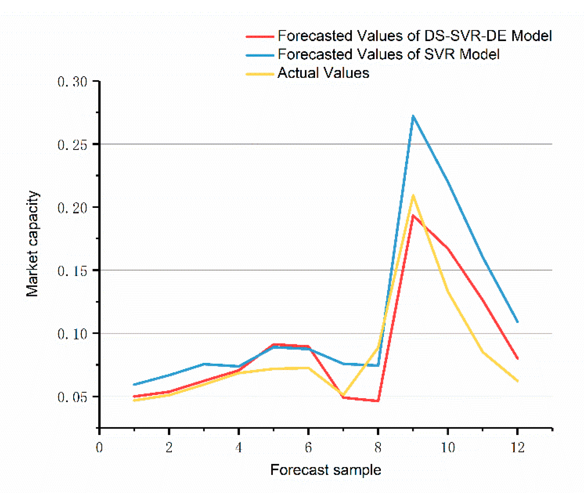
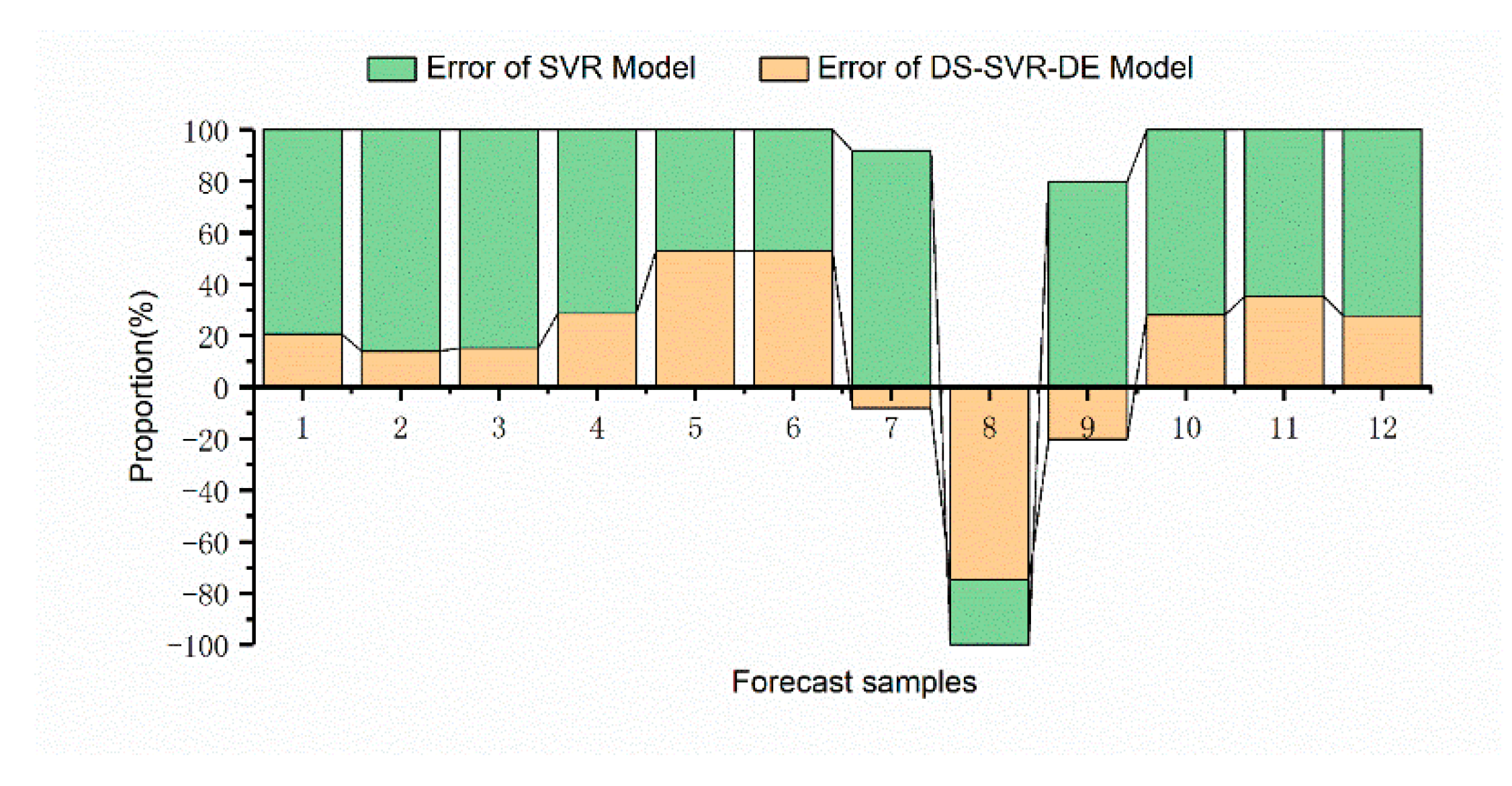
3.3.1. Discussion on the Long-Term Forecasting Results
We discuss the method of long-term prediction part in the decision-making framework with SVR model based on decomposition strategy that we proposed. Then compare the results with the SVR and SARIMA on the forecast set. Their performance is shown in
Figure 4 and
Figure 5.
Table 6 gives the demand analysis results of those models.
According to the results, the proposed long-term forecasting method is similar to the traditional forecasting methods in the test set. However, the extrapolation error of the proposed method in the prediction set is obviously smaller. Additionally, the monthly error ratios of the two models show that the proposed DS-SVR model is lower, which can be explained theoretically. The DS-SVR model limits the effects of various factors on the market to each subinterval in the process of feature analysis, thus reducing over-fitting errors that may occur in the actual training process. Moreover, the two methods are well in line with the general trend of the construction machinery market in the long-term forecasting process.
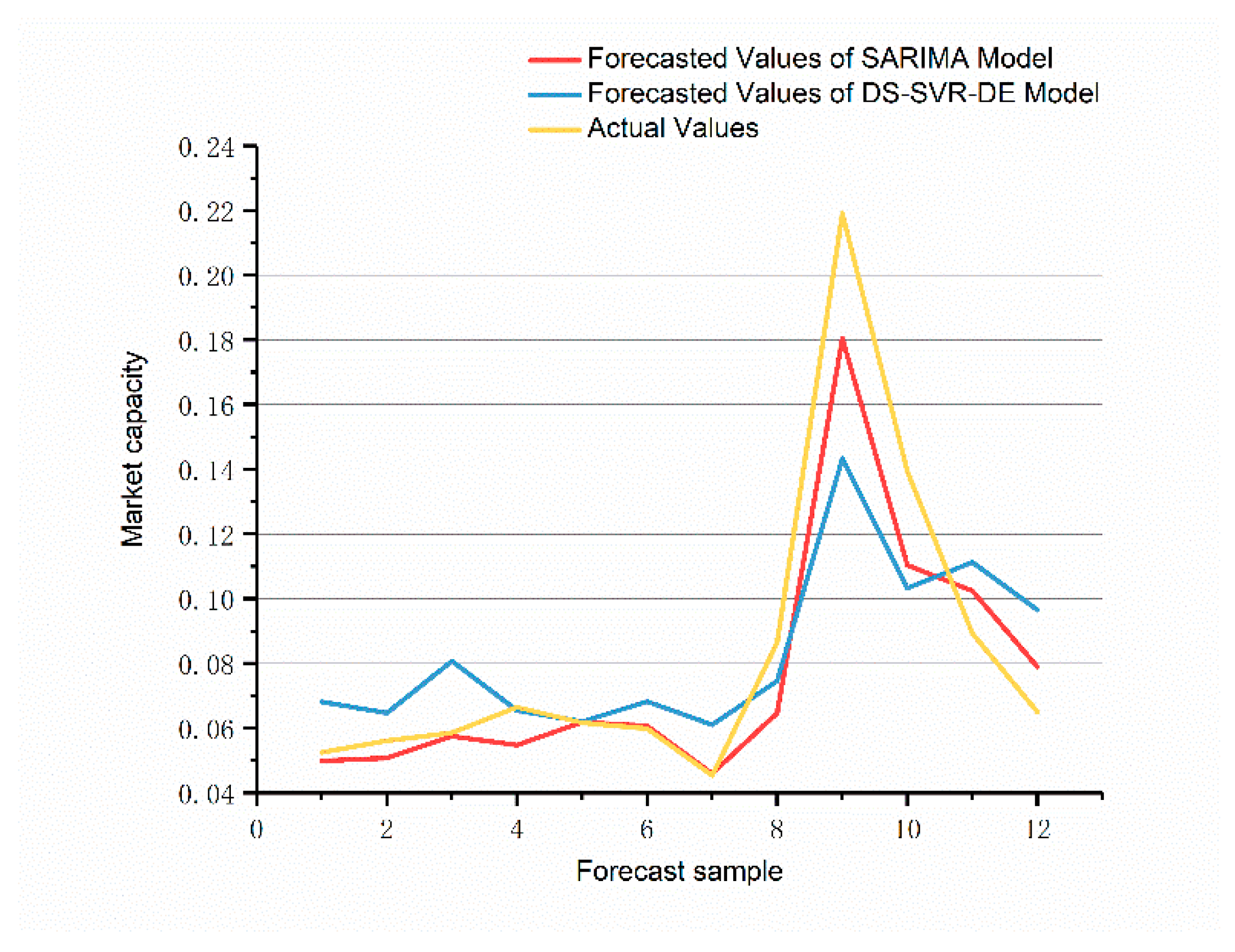
Then, the forecasting results are compared with the seasonal method of the ARIMA model, and the final effects of long-term prediction are verified. The test is conducted with the medium-sized case, which is more complicated than the other two types.
Figure 6 and
Figure 7 show the experiment results.
It can be seen that both DS-SVR and SARIMA can follow the changing trends of the market in long-term forecasting. However, the overall performance of the SARIMA model on the prediction set is biased to one side, while the DS-SVR model is closer to the actual situation. The prediction RMSE of the SARIMA model on the prediction set is 1515, and the prediction RMSE of the DS-SVR model is 1209. For the long-term prediction, the DS-SVR model results are significantly better than SARIMA. On the other hand, the SVR method based on multi-source data analysis is theoretically more reliable, which is reflected in the face of abrupt changes in upstream and downstream industries and the impact of national financial policies.
3.3.2. Discussion on Short-Term Forecasting Results
In this section, the periodic conditions for applying the algorithm to short-term prediction are discussed based on the ARIMA model. Then the proposed improved model is adopted and compared with SVR and ARIMA models.
Relevant studies show that the forecasting accuracy of SARIMA is affected by the number of periods in the lag time series. Therefore, the relationship between the number of periods in the forecasting time series and the forecasting accuracy is further explored in the dataset.
Figure 8 shows the relationship between different forecasting periods.
According to the results, with the same input sample, the training error and the prediction error have tendencies to increase with the increase of prediction periods, which is also in line with the characteristics of the autoregressive model affected by the number of lag periods and further illustrate that ARMA model is not suitable for providing long-term decision support. In this case, it is necessary to find the best autocorrelation lag time in use. The error of this research model in three months has basically met the demand, and shorter forecast periods are worthless to the implementation of production lines. Therefore, the optimal results are used to set the number of short-term prediction lag periods and compare them with the SVR algorithm again.
Figure 9 shows the comparison curves. The results of quantitative analysis in RMSE show that the prediction error of SVR is 1596, and the prediction error of SARIMA is 933. The results show that the SARIMA has better short-term forecasting accuracy (
Figure 10).
To sum up, SVR results are significantly better than SARIMA for long-term prediction. On the contrary, SARIMA has achieved better results in short-term prediction.
3.3.3. Modified Method for Short-Term Forecast
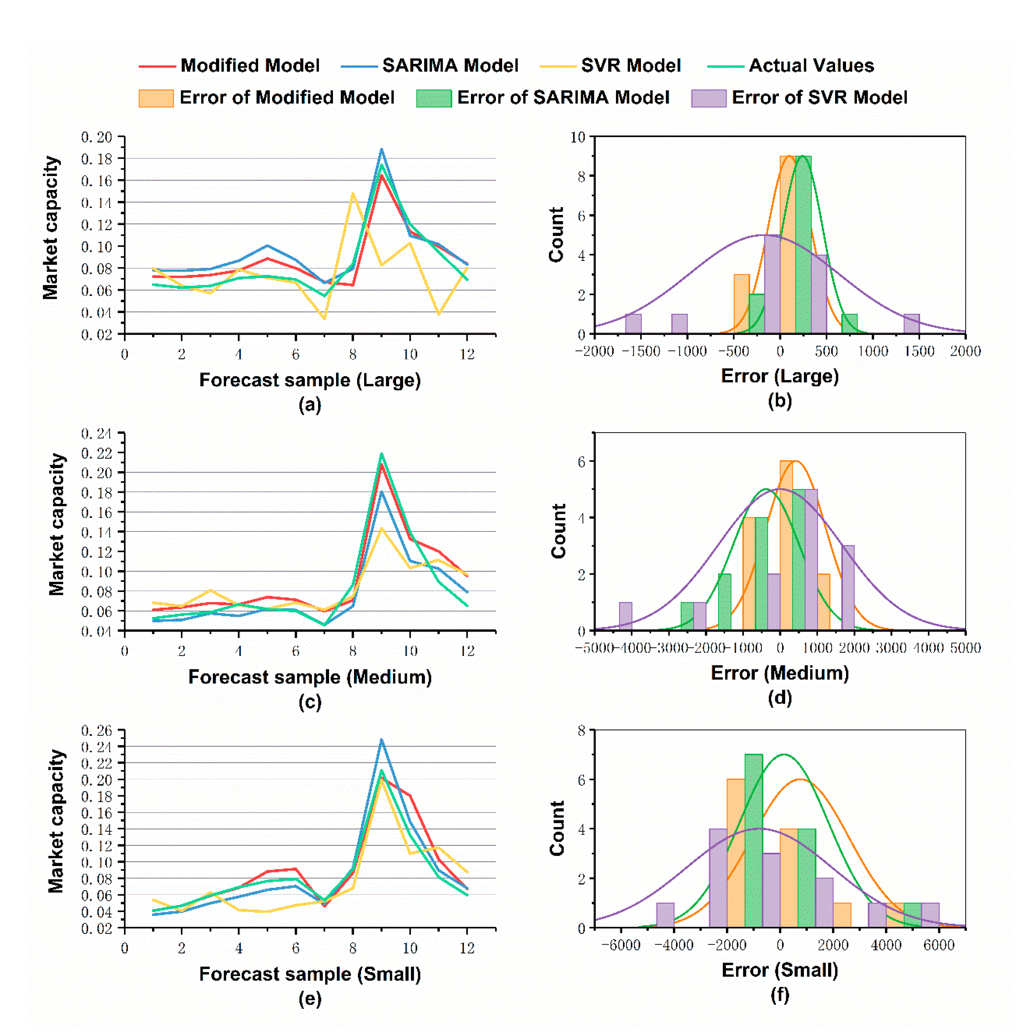
Although the seasonal ARIMA model has achieved good results in short-term forecasting, it has limitations. The multi-source data-driven forecasting method has better application prospects. Therefore, a modified model and forecasting process is proposed for further study of the short-term forecasting effect of the decision framework aiming at overcoming the limitations. In particular, this study applies the previously drawn conclusions, including the forecasting effects and enterprise production scheduling, to set the number of forecasting periods to three periods and adopt a modified model of decomposition method to achieve decoupling between multivariate factors. The results are shown in
Figure 11.
Comparing the SARIMA, the SVR, and the modified forecasting algorithm,
Figure 11 shows that the short-term market capacity prediction on large, medium, and small excavators basically conforms to the data change trend, and the SVR effect is slightly poor. Residual analysis indicates that the prediction error follows Gaussian distribution, and the average value will tend to zero under the condition of large samples. It verifies the reliability of the model. In the market capacity forecasting of large and medium excavators, the modified algorithm performs better, and the error distribution tends to zero. The qualitative analysis in
Table 7 has reached the same conclusion. The RMSE and error rate of the ARIMA, SVR, and modified model on the forecasting samples decrease in turn according to the law of small to large. The MAE and MAPE also basically conform with this trend. The modified model is superior to the ARIMA model and epsilon–SVR model on the prediction ability of medium and large scale, while the ARIMA model has better performance on the small-scale type.
However, simply using the SARIMA model cannot capture the nonlinear relationship in market changes in principle. On one hand, it cannot resist the influence of market risks and financial policies, which means it has certain limitations in reliability. In this case, the SARIMA model on the random offset of the error mean in
Figure 11 is larger than the modified model. For further analysis, the limitation is because the SARIMA model cannot capture the nonlinear causality of market changes well; thus, this part of the information is “leaked” into the residual error. In contrast, the modified algorithm integrates data-driven analysis technology and can recover this part of information through multiple data regression. Therefore, it is considered to be a more scientific way to consider the long-term SVR forecasting results comprehensively.
At the same time, it can be seen from
Table 8, for the short-term modified forecasting algorithm, the coefficient of the SARIMA model is higher than the SVR model. It is the optimized result by the DE algorithm. It can be seen that the model values more of the data results in short-term prediction and also considers the influence of epsilon–SVR.
To sum up, the DS–SVR–DE model for long-term prediction has a stronger prediction ability than the SARIMA model and SVR model. Its application in enterprises will play a supporting role in the long-term market decision. In view of the fact that the short-term forecasting modified algorithm is better than the SARIMA model and SVR model, which can capture the nonlinear changes of the market, the modified model is adopted for short-term forecasting to provide support for actual order production.
4. Conclusions
According to the characteristics of the construction machinery industry, the long-term and short-term forecasting model is proposed in this paper, which is dedicated to solving the production decision-making problem of enterprises under market behavior and also is used to build enterprise production decision support systems.
First of all, a framework of a complete market decision-making system model is proposed. Then, the market forecasting method based on the combination of long-term and short-term is discussed, which includes a long-term forecasting part with a step length of 1 year and a short-term forecasting part with a step length of 3 months.
Among the framework, the long-term forecasting of market capacity is studied based on the DS-SVR prediction model. Monthly data from 2006 to 2019 are collected to support the forecasting work. The forecasting method based on decomposition synthesis RBF is proposed to select affecting factors and the differential evolution algorithm to optimize the model. The long-term forecasting model is proposed to compare with the SVR model and SARIMA model. The results show that the mean error rate of the proposed decomposition-synthesis prediction method on the forecasting set is 26.61%, which has higher accuracy than SVR or SARIMA.
On the other hand, the short-term forecasting method is studied. Based on the original training set data, the SARIMA model is tested with different time series lag periods. The results show that the forecasting accuracy of excavator sales decreases with the increase of lag periods. In principle, the delay time is shorter, and the effect is better. Therefore, a short-term forecasting model with a prediction step length of three periods is established. Through the practical verification, the decomposition error rates of the SARIMA model on the forecasting set are 17.92%, 20.02%, and 16.55%, and the SVR model is 44.98%, 34.24%, and 28.18%. The results show that the SARIMA model has better short-term prediction accuracy than the epsilon–SVR model.
Furthermore, the improved short-term prediction algorithm is proposed based on the SARIMA and epsilon–SVR, and the differential evolution algorithm is applied to optimization. Through practical verification, the decomposition error rates of the improved short-term prediction algorithm are 13.65%, 18.83%, and 19.62%, respectively. The results show that the prediction accuracy of the SVR–SARIMA composite model is better than the SARIMA model. Moreover, we found that the short-term forecasting coefficients distribution with the improved algorithm is more inclined to the SARIMA algorithm, which showed there exists a strong autocorrelation and trend of construction machinery market. Meanwhile, multivariate regression data are also taken into account to a large extent by the algorithm at the same time, which is considered to have a major impact on the volatility and amplitude of the construction machinery market.
According to the results, the long-term and short-term forecasting methods can well reflect monthly data changes from the trend, but the accuracy of the long-term and short-term forecasts still needs to be improved in further studies. It is believed that the proposed method has great value to be applied to the construction of enterprise production decision support models. The research also has some limitations. Due to various factors affecting the construction machinery industry, only parts of upstream and downstream industrial factors are considered in this study. Some nonquantitative factors are failed to analyze effectively. For further studies, the complexity of the model and the training period should be further upgraded, and more relevant factors should be tested and quantified to improve the performance of the model.


 ,
, 


