Abstract
A preventive maintenance embedded for the fused deposition modeling (FDM) printing technique is proposed. A monitoring and control integrated system is developed to reduce the risk of having thermal degradation on the fabricated products and prevent printing failure; nozzle clogging. As for the monitoring program, the proposed temporal neural network with a two-stage sliding window strategy (TCN-TS-SW) is utilized to accurately provide the predicted thermal values of the nozzle tip. These estimated thermal values are utilized to be the stimulus of the control system that performs countermeasures to prevent the anomaly that is bound to happen. The performance of the proposed TCN-TS-SW is presented in three case studies. The first scenario is when the proposed system outperforms the other existing machine learning algorithms namely multi-look back LSTM, GRU, LSTM, and the generic TCN architecture in terms of obtaining the highest training accuracy and lowest training loss. TCN-TS-SW also outperformed the mentioned algorithms in terms of prediction accuracy measured by the performance metrics like RMSE, MAE, and scores. In the second case, the effect of varying the window length and the changing length of the forecasting horizon. This experiment reveals the optimized parameters for the network to produce an accurate nozzle thermal estimation.
1. Introduction
The innovative way of production method operated by additive manufacturing (AM) or 3-D printing takes the manufacturing process in a whole new perspective [1]. With this emerging technology, engineers are up to challenge in transforming their concept on designing a product and at the same time, it is a chance to showcase their creativity in solving modern engineering problems. AM unlocks endless possibilities towards the manufacturing scene; stretching its accessibility even in remote places, while radically reduces manufacturing time, cost, and material waste. Those attributes gained the attention of multi-disciplinary field to adapt this emerging manufacturing technology. For example, in aerospace sector, additively manufactured rocket engine [2], astronauts utilize 3D printers on an in-space manufacturing [3], and even looking at the feasibility in manufacturing food during space flights [4]. Another is the use of AM manufactured scaled model to measure the integrity of building designs [5], printing antenna [6], electrical circuits [7] and revolutionizing modern medicine with tailored bio-printed products [8]. Although there are countless applications of additive manufacturing, there are underlying issues on printing reliability [9] and quality of the fabricated product [10].
For instance, in one type of printing technique called fused deposition modeling (FDM) wherein the object is built layer-by-layer out of melted polylactic acid (PLA), the products became susceptible on having anisotropy in their mechanical structure mainly attributed on overlooking the influence of the printing mechanism to the intrinsic properties of the filament [11]. One of the notable printing parameters is the extrusion temperature whereas due to unstable or extreme temperatures, it drives a disproportionate curing and melting rate of the quasi-solid material that results in poor layer bonding between adjoining layers, prominently reducing the mechanical strength of fabricated products [12,13], leads to physical deformation [14] and porosity [15,16]. These mentioned degradation on product quality are still in need of monitoring system [17]. Additionally, aside from affecting the rheological properties of the material, the nozzle temperature also influences the velocity of filament extrusion, a critical factor attributing on nozzle clogging that can cause a printing failure [18,19]. Aware of this, researchers focus on building monitoring systems and adaptive controls aiming to prevent degradation in product quality or printing failure before it happens.
Developments in monitoring system includes techniques like modelling the mechanical aspects of the extruder [20,21,22,23] to further build a digital twin of the printing process adopted by [24]. To predict the filament’s temperature, the researchers implemented an algorithmic resolution procedure, and thresholding method, respectively. In predicting the interfacial temperature interaction between the melted PLA and the previous layer a linear Kalman filter estimation is used [25]. A different approach is done in [26] where the thermal state of the nozzle has been estimated using a multiphysics simulation software. These techniques provide precise nozzle temperature predictions however, the mentioned procedures are relatively slow for real-time applications.
To reduce these gap, recent studies focus on machine learning-based monitoring system have been developed. There are studies that classifies faulty fabricated products using support vector machines (SVM) like in [27] where a thermal imaging camera are utilized. A similar approach is adopted in [24] as infrared thermal imager acquired the nozzle temperature, and a qualitative trend analysis is used to extract sensitive feature parameters and based on the extracted values, warping on the product is identified using thresholding method. Although the papers provided accurate monitoring and identification of the anomalies during the printing operation, the defects and degradation on fabricated products are yet to be prevented. On that note, closed-loop control and monitoring platforms are proposed. On [28] a cyber-physical system (CPS) can provide an online data user interface where the printing parameters are displayed and according to the authors, they used SVM to extract the data features and a PID control is responsible to stabilize the nozzle temperature. They presented a promising technology; however previous studies have succeeded controlling the nozzle temperature by using PID control itself [29] and from the mentioned papers the existing monitoring and quality control program was able to detect the anomaly during or moments before it occurs making it difficult to prevent the fault from occurring. To overcome this, an artificial neural network-based monitoring system embedded for the FDM printing technique is proposed in this paper.
Distinct from the presented papers, our proposed monitoring program provides a nozzle thermal estimation in future time-steps. The use of artificial neural networks in forecasting is becoming a trend in predictive maintenance [30] and have also been applied on other fields [31,32]. The forecasted values are processed on an anomaly detection intended to detect possible irregularity on the nozzle temperature values that can lead to thermal degradation on the fabricated products as well as probable nozzle clogging that is one of the prominent printing failures in this type of printing technique [31]. A temporal convolutional network with a two-stage sliding window strategy (TCN-TS-SW) is proposed to perform the thermal estimation. TCN-TS-SW’s ability to perform parallel computations that requires low memory for training is seen as an advantage towards the working environment that is presumed to receive a long sequence of data. To further reduce inference time and memory consumption, an initial sliding window technique to execute a coherent pre-processing procedure to improve the time series forecasting.
2. Proposed Methodology
In building a monitoring system for a FDM 3D printer a temporal convolutional network with a two-stage sliding window strategy (TCN-TS-SW) is proposed to perform the estimation on the thermal state of the nozzle tip. This architecture is inspired by the temporal neural network (TCN) presented in [33], an artificial neural network architecture originally built to perform sequence modelling just like Nonlinear Autoregressive Neural Network with Exogenous Input (NARX) [34], LSTM [32] and CNN [35]. The temporal convolutional network (TCN) overcome the drawbacks of the canonical RNN on vanishing gradient problem. However, one of the major disadvantage TCNs compared to RNN is the higher memory footprint during inference to compromised with that, we propose a two-stage sliding window to execute a coherent pre-processing procedure to improve the time series forecasting.
In this approach a one-dimensional time series data is collected from the thermal readings at time t such that, x is the input of the system. The effectiveness of the proposed scheme to forecast the potential values of the temperature measurements at time i is denoted by , where h is the prediction horizon. In case that the values in y follows a critical trend, the control system issues a halt on operation. In this countermeasure, the aim is to stabilize the nozzle temperature preventing the degradation on the fabricated product that is bound to happen.
2.1. Two-Stage Sliding Window Strategy
In the data pre-processing part, the samples in the dataset were first assigned to the training set and validation set. In the proposed two-stage sliding window strategy, the initial execution is performed on the elements of both training and validation set. The elements is split into fixed-length sequences using a time window of length () with sliding step of () as shown in Figure 1a. The process continues until the last value of the series is segmented. The split-sequence is matched to the predefined level of unfolding to transform x into a two-dimensional vector. The values for and were selected considering the sampling capacity of the data acquisition module, as well as the printing speed. This network parameters are applicable on the first and second case studies conducted on the performance evaluation. The second stage of the sliding window technique shown in Figure 1b is performed on the training set split sequenced to define the forecasting interval h which is calculated through the difference of the shift between m and target series. This technique achieves less error approximation and achieves better prediction performance as concluded in [36].
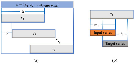
Figure 1.
The two-stage sliding window strategy. (a) The first sliding window performed on the training set. The data involved are to , which is the last element of the training set. It has a time window length, and sliding step, , and the split segment are indicated by up to , the last segment containing . (b) Segment is segmented by m is the input length and target series bearing the forecasting interval h.
2.2. Structure
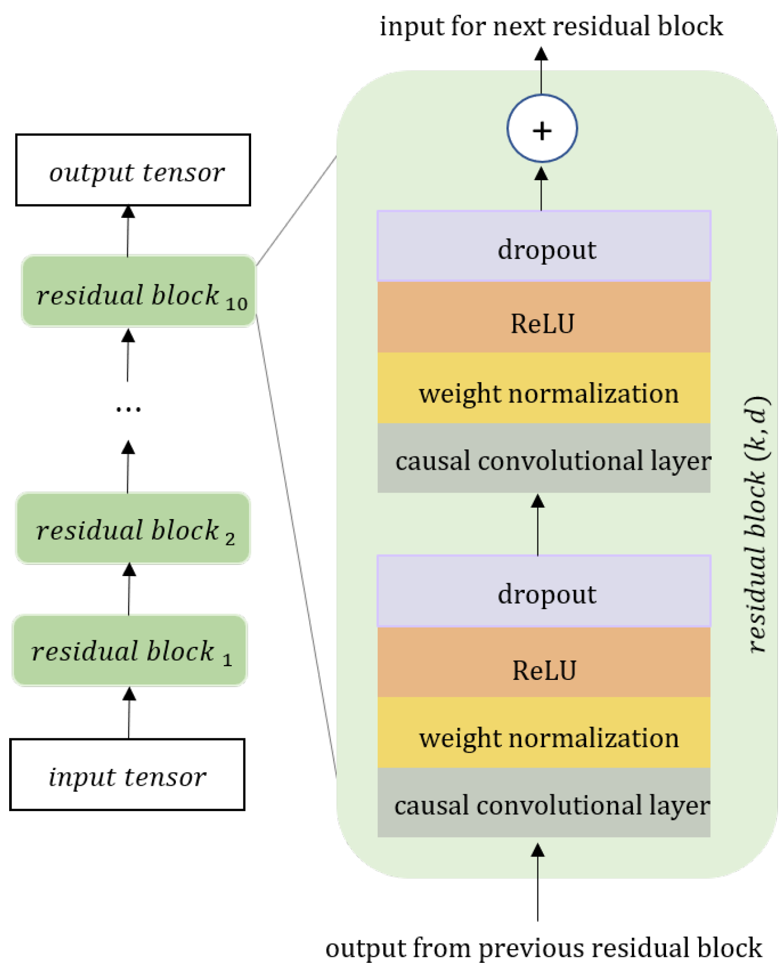
The forecasting model is composed of layers of residual blocks made up of stacked dilated convolution layers, non-linearity functions, and dropout layers. The overall architecture is illustrated in Figure 2. Instead of utilizing causal one-dimensional convolution, these residual blocks are used to ensure that the forecasted values solely depend on the series’ history values, x. In order to maintain the same length between the input and output, zero-padding is added on input to ensure the uniformity of length in each layer and it also applies on the successive layers of the dilated convolutional layer present on the residual blocks. Dilated convolutional layer replaces the conventional convolutional layer because dilation increases the input’s receptive field while maintaining the number of layers relatively small. In choosing the minimum number of residual blocks that guarantees that the output sequence utilized full history coverage, can be computed as:

Figure 2.
The temporal neural network architecture. It includes a total of residual blocks, receptive field , dilation base and the kernel size .
The dilation base is an integer whereby dilation refers to the space between the input elements on each layer l of a convolutional layer, m is the input length. In the equation, k is the kernel size of which is the length of sequential elements in the input. These series of elements with length k are multiplied with a kernel vector of leaned weights of the same to get the input of the proceeding layer. The output of the causal convolution layer is normalized using weight normalization and further transformed to learn the non-linear representation of the data using the rectified linear unit (ReLU) function. To safeguard the model from overfitting, a dropout layer is introduced at the end of the convolutional later of the residual block. Note that in the final output of the model, the ReLU is deactivated for y to take on negative values as well.
The time-series output y is subjected to predictive anomaly detection through threshold classification. The control system is designed to counteract the two possible scenarios:
- The predicted nozzle temperature is below the normal printing temperature which is from 185 C to 220 C [37]. This case happens due to the filament flow rate is high, and the nozzle begin to drop its temperature due to heat transfer between the filament and nozzle. The operation will partially halt giving time to the nozzle to stabilize its temperature.
- The temperature of the nozzle is above the normal printing temperature: In contrast to the first scenario, the action taken by the control system will be the activation of fan to cool the nozzle. This action is taken to stabilize the normal printing temperature range mentioned.
3. Experiment Setup
This section discusses the hardware and software used for the data gathering and the methodology used to perform the nozzle thermal estimation. Also, for testing the performance of the proposed TCN-TS-SW algorithm, two experiment set-up is conducted.
The actual set-up is presented in Figure 3. The experiment set-up includes a cartesian FDM printer single extruder system (EDISON multi) with a single extruder system and the nozzle attached has a size of 0.4 mm diameter. The printing bed has an initial pre-heated temperature of 90 C. The summary of the printer specifications are listed in Table 1. The sensor is selected based on the consideration the enclosed FDM printer structure of EDISON Multikit, thermocouple is a suitable sensor to provide precise temperature reading without depending on any external factors like light sources. It is capable of measuring up to 350 C and can withstand the high working temperature of the nozzle. The sensor is connected to a cold junction-compensated K-Thermocouple to-Digital converter (MAX6675) (Kuongshun Electronic Limited, Manufactured in Guangdong, China) which is capable of data output in a 12-bit resolution, 0.25 C resolution. The MAX6675 module is then connected to the Arduino Uno device as the data acquisition module.
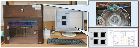
Figure 3.
The experimental set-up for the data acquisition and process monitoring.

Table 1.
3D Printer Experimental conditions.
Then, the Arduino uno is connected on the desktop computer by a serial connection. The maximum sampling rate for Arduino uno is 400 samples per second. The aggregated sensor readings are then saved on an edge device in comma-separated value (.csv) format that is utilized for the machine learning processing. The software used in this project are the following: LabVIEW 2020 for data logging and en-thought python integration toolkit is used to process the data for machine learning prediction integrated on the LabVIEW program. The TCN model that was utilized in this paper is based on the [38] and was compared to model [39].
The proposed system, a uniform specimen is printed during the experiment. The ASTM D638 type I, is a standard specimen created to perform the tensile test method for polymers. These are printed to perform uniform comparison throughout the experiment. The specimen has a dimension of (165 mm × 19 mm × 13 mm). The file designed in stereolithography file (.stl) and is later converted on the employed FDM printer’s compatible file format (.x3g).
4. Performance Evaluation
This section is going to discuss the performance of the proposed TCN-TS-SW in the following case studies:
- The validation of TCN-TS-SW versus other machine learning (ML) algorithms like multi-look back LSTM, LSTM, GRU in terms of training loss and training accuracy.
- The effectiveness of the proposed two-stage sliding window technique is investigated as the proposed scheme is compared to the classic TCN model presented in [33] in terms of training loss and accuracy.
- The forecasting capability of the TCN-TS-SW. The results are presented using performance metrics like RMSE, MAE, and and the predicted data is plotted againts the actual data.
Also, it is an important note that in every experiment conducted, there are different set of data are utilized and, in each section, the structure is be explained. To analyze whether the proposed architecture is performing well in terms of accurately providing the forecasted nozzle temperature values, the models presented in this paper were evaluated using the metrics like root-mean-square error (RMSE), mean absolute error (MAE) and .
Presented in Equation (2), RMSE is the squared-root value of mean squared error that reveals the deviation between the actual temperature reading to the predicted data at time i, and N is the total number of observations involved. Another metric is the mean absolute error (MAE) in (4), that asserts the absolute average residual between and . Lastly, r-squared or the coefficient of determination in Equation (4), is an indication of how well the predicted values replicate the actual observation. The values of can be on the less than zero [40].
4.1. TCN-TS-SW versus Other Machine Learning (ML) Algorithms
To evaluate the performance of the proposed TCN-TS-SW in terms of training loss value as compared to other machine learning algorithms namely multi look-back LSTM (MLB-LSTM) [32], gated recurrent unit (GRU), and LSTM. A dataset is accumulated by utilizing the experiment setup described in Table 1. Note that the sampling rate of Arduino uno is set to 3000 samples/min. As a result, the dataset contains 328,470 samples from just over 109 min of execution time. It is then assigned to the training set and validation set on a 75/25 ratio.
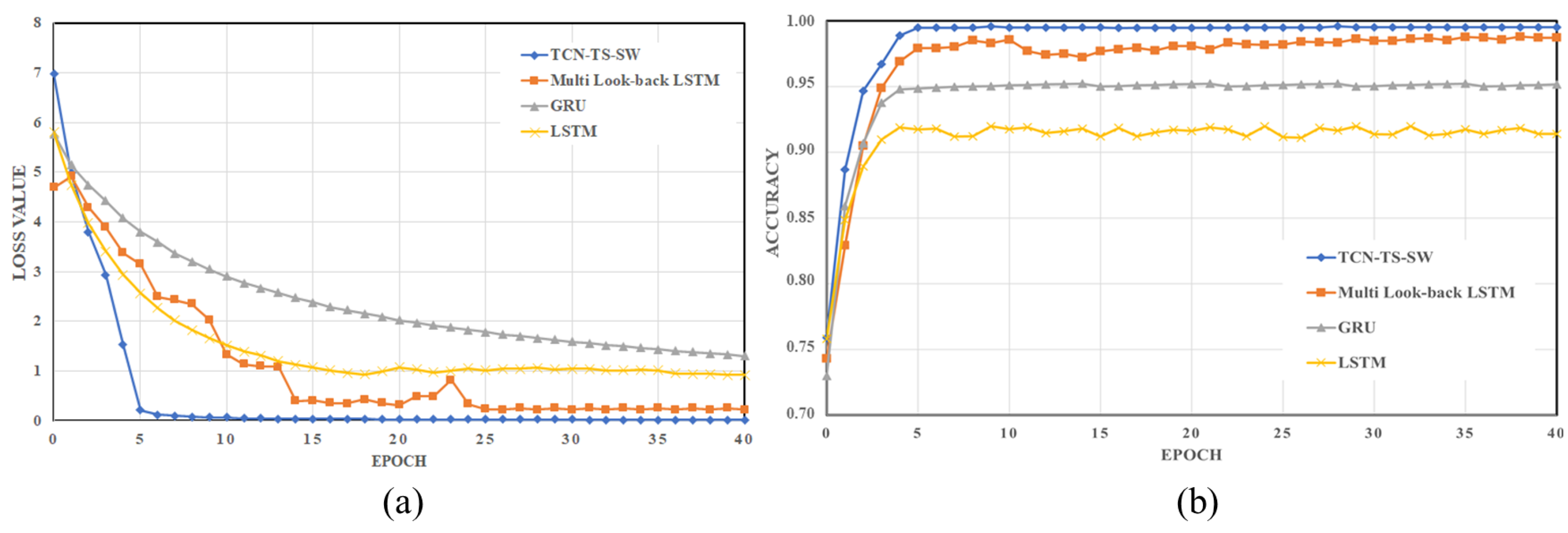
The performance of the proposed TCN-TS-SW in terms of training loss value as compared to other machine learning algorithms namely multi look-back LSTM (MLB-LSTM) [32], gated recurrent unit (GRU), and LSTM is presented on the Figure 4a.
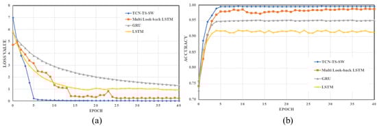
Figure 4.
The performance of TCN-TS-SW against the multi look-back LSTM, GRU, and LSTM. (a) Time-series training loss over epoch. (b) Time-series training accuracy over epoch.
The results showed that TCN-TS-SW reaches the lowest training loss value over 40 epochs, and a good performance in terms of accuracy is illustrated in Figure 4b. Although the proposed scheme’s loss is the highest in the first epoch, it was able to converge with the lowest training loss after 40 epochs, outperforming the MLB-LSTM, GRU, and LSTM.
As presented in Table 2, the proposed TCN-TS-SW resulted to the lowest RMSE and MAE values which indicates a good fitting prediction model. The proposed model also got the highest r-squared score indicating a low variation between the forecasted values compared to the actual temperature readings, outperforming the other algorithms in all performance metrics presented.
Table 2.
Comparison Results for RMSE, MAE, and .
4.2. Generic TCN versus TCN-TS-SW
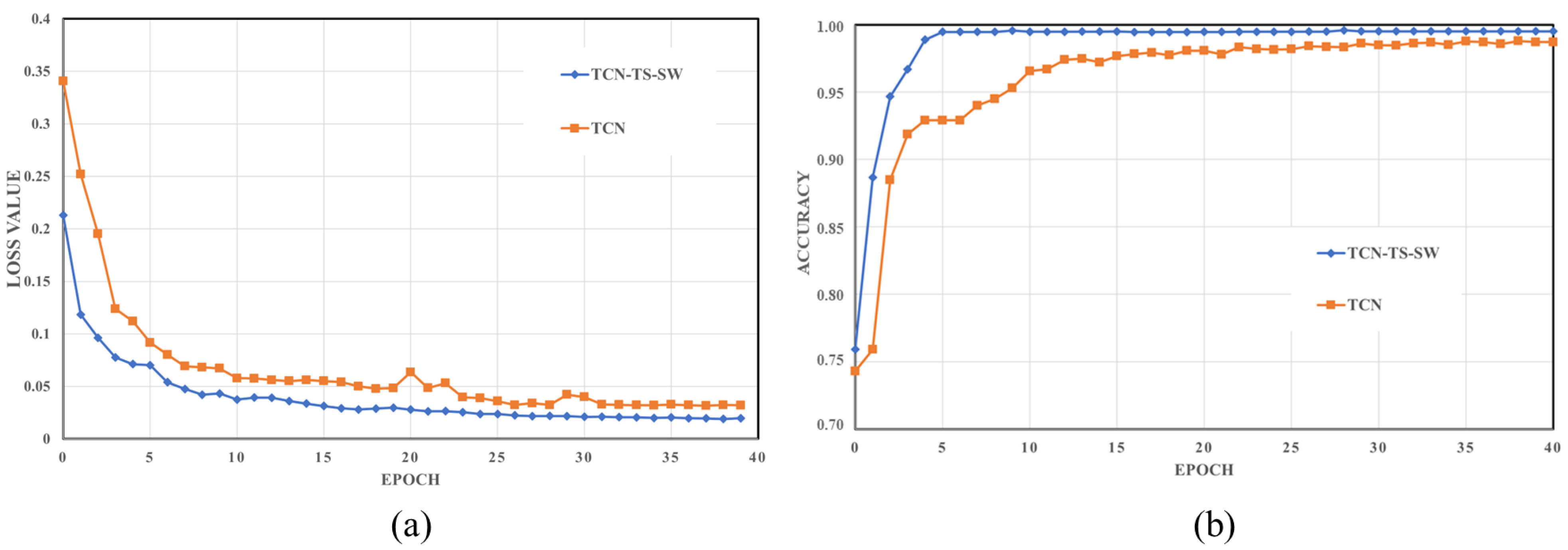
To evaluate the performance of the proposed TCN-TS-SW with that of a normal TCN model [39] comparative study is presented. The effectiveness of introducing the two-stage sliding window strategy to the TCN model is observed to minimize the training loss as shown in Figure 5a and also increases the accuracy of prediction implicated by the results shown in Figure 5b. The figures both showed the effectiveness of two stage sliding window strategy implementation to that of a traditional TCN model.
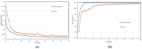
Figure 5.
The effectiveness of two-stage sliding window strategy when applied to the temporal neural network architecture. (a) The proposed scheme’s vs TCN in terms of training loss over 40 epochs. (b) The effectiveness of the proposed system versus the later in terms of training accuracy.
4.3. TCN-TS-SW Forecasting
In this experiment, the effect of adjusting the time window length is investigated. Also, in this section, it will highlight the justification of the reason behind the proposed two-stage sliding window technique.
A different dataset is used in this experiment and follows the setup as specified in Table 3 however, the sampling rate on the data acquisition device is adjusted to 400 samples/second. Note that the sample acquisition is conducted within 5 s interval. The dataset is composed of raw sensor readings from the acquisition device, hence the temperature readings are still on voltages. For uniformity, the same set of dataset is used all throughout the experiment.
Table 3.
TCN-TS-SW System Parameters.
The TCN-TS-SW can compute for the historical forecasts the model that returns a time series created from the last point of each of these individual forecasts. It trains the current model on the training set, emits a forecast of length equal to forecast horizon, and then moves the end of the training set forward by stride time steps. The term start, refers to the first point of time at which a prediction is computed for a future time-step. The numerical value pertains to the proportion of the series that should be present before the first prediction point.
In building the forecasting parameters of the model: we need to define that the m = start * . Input length refers to the past time steps that are fed to the forecasting module. Discussing further, a window length of and start = 0.8 then, the input length , that is also equal to the length of target series (refer to the Figure 1). With that determined, the number of elements forecasted, forecast horizon h is equal to h = (1 − start) * referring to the number of elements that is forecasted in one loop of execution.
For the scenario I structure, it is summarized in Table 3. The window size and note that is equal to . For the second stage of sliding window technique, the training and validation data is split to 70-to-30 percent ratio. Note that this ratio does not affect the activity of the sliding window technique. The random state value refers to the degree of randomness of the initialized weights. This network characteristic contributes as a factor on the difference on the simulation results. The training epoch is set to 5 and it trains the current model with the training set, emits a forecast of length equal to forecast horizon, and then moves the end of the training set by stride time steps. For the residual blocks: the kernel size is equal to 3, number of filters is equal to the number of residual blocks necessary to achieve full receptive field coverage, computed using the Equation (1). Finally, the dropout rate is applicable for every convolutional layer throughout the network.
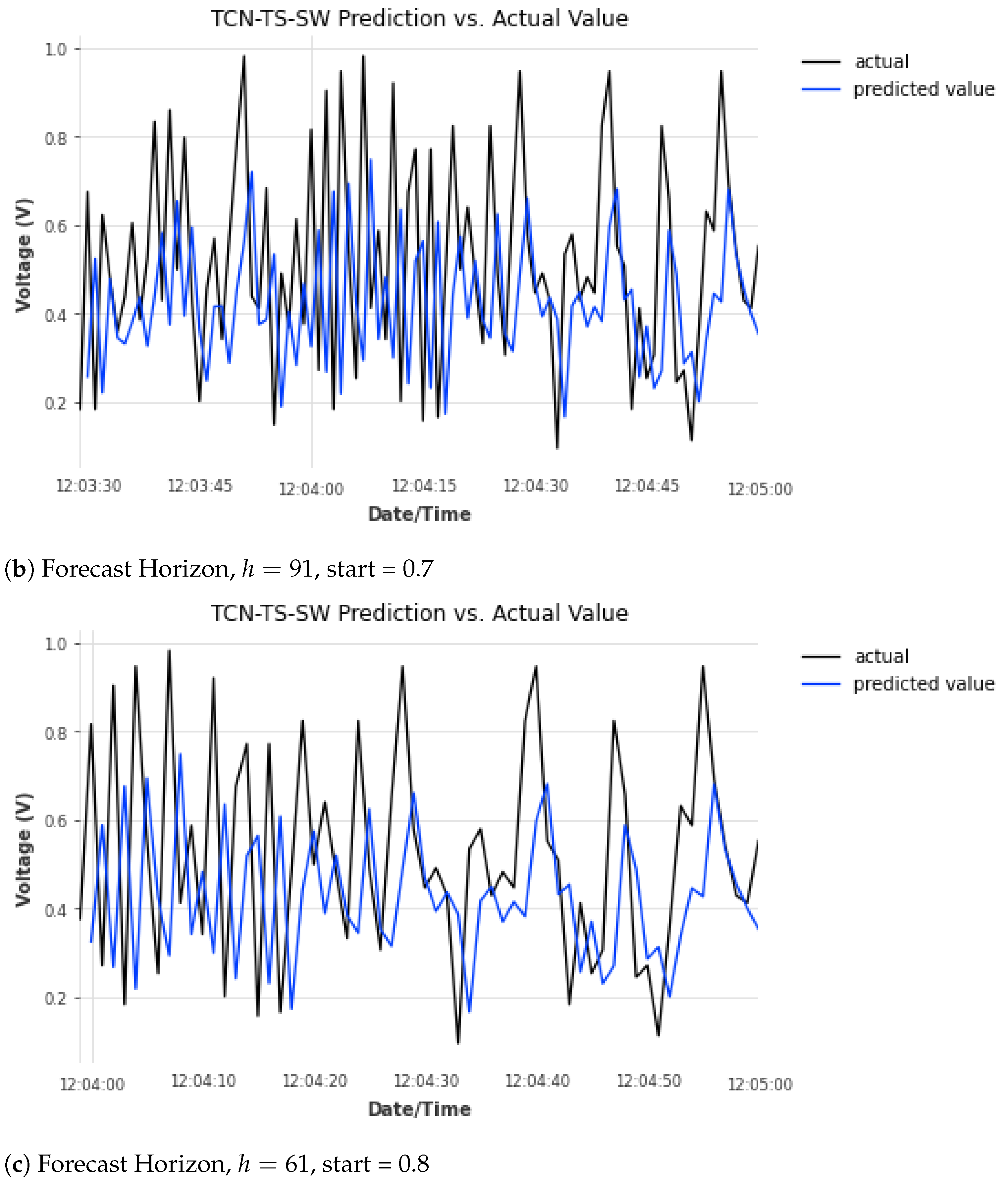
As can be seen in Figure 6 the alongside comparison of the actual data versus the predicted one. The forecasting module of the proposed TCN-TS-SW performs satisfactorily to reproduce the actual data. It is because of a low number of epoch and a relatively small number of training data. The reason behind choosing a low epoch number is that since we are considering a real time application, the execution time would be the highest priority in designing the this structure in return, the accuracy is compromised. For further validation, the accuracy of the proposed system is evaluated by the RMSE, MAE and score metrices summarized in Table 4. The window size variation of display the best setup for a single stage sliding window technique is observed in the data ratio of 0.6. However, it is observed to have a negative score and this event can be traced back to the data presented on this model. The nature of the time-series subjected to our proposed model; TCN-TS-SW, is an irregular trend that does not include any seasonality or uniformity. It consist of gross outliers that could contaminate the fairness while computing the resulting a negative value on the final output. Additionally, the decremented of accuracy is caused by uncertain noises and dynamic variance of input data.
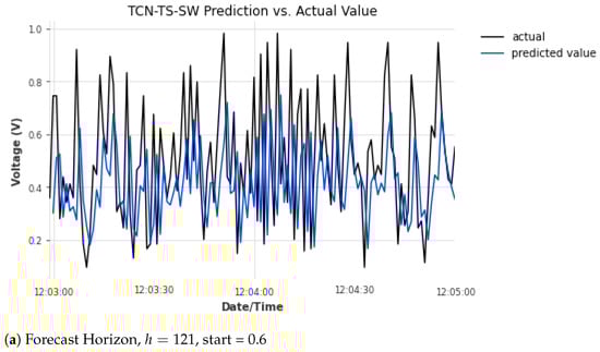
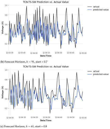
Figure 6.
The plotted result between the actual and predicted values. The network has a with a training/validation ratio of 70/30. The x-axis represents the time of the execution, and the y-axis represents the voltage (Volts) that represents the raw readings from the temperature sensor.
Table 4.
Comparison Results for RMSE, MAE, and .
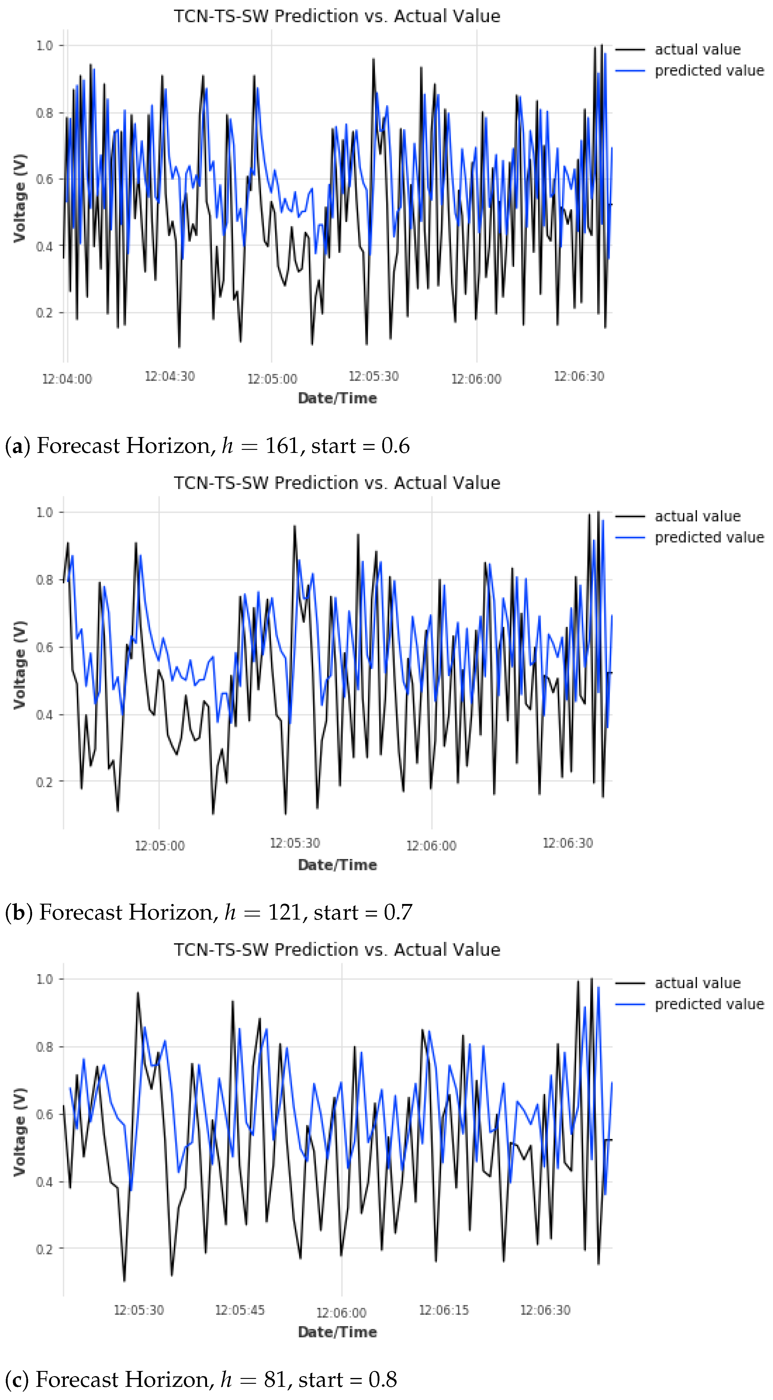
Meanwhile for can be seen on the Figure 7 the alongside comparison of the actual data versus the predicted one. The forecasting module of the proposed TNN-TS-SW performs better compared to the since there are relatively more training dataset involve during the training procedure. For further validation, the accuracy of the proposed system is evaluated by the RMSE, MAE and score metrices summarized in Table 4. It shows that the best setup for a single stage sliding window technique is observed in a starting ratio of 0.6 and a forecast horizon of 161 elements. However, it also have a low score similar to the result from the first scenario hence, it also implicate a huge variance between the actual and predicted value hence, the result of having a negative value is due to the absence of constant term on the (4) as further explained on [40,41].
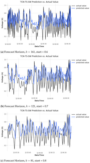
Figure 7.
The plotted result between the actual and predicted values. The network has a Δ = 400 with a training/validation ratio of 70/30. The x-axis represents the time of the execution, and the y-axis represents the voltage (Volts) that represents the raw readings from the temperature sensor.
5. Conclusions
To build a robust predictive maintenance system for fused deposition modeling (FDM) in additive manufacturing, the authors proposed TCN-TS-SW to accurately provide a nozzle thermal prediction for the monitoring program. The simulation results proved that the proposed two-stage sliding window strategy elevates the prediction robustness and minimizes the training loss against the generic temporal neural network. In addition to that, TCN-TS-SW outperformed the other machine learning algorithms namely multi look-back LSTM, GRU, and LSTM in terms of accuracy and training loss. The statistical performance evaluation for regression; root-mean-squared error (RMSE), mean absolute error (MAE), and is used to display the robustness of TCN-TS-SW in providing an accurate predicted values compared to other models. The effect of modifying the window length is also investigated and through the conducted experiment, displays more accurate prediction compared to window length in terms of RMSE, and MAE. However, both scenario received a negative that implies a high variance between the predicted values versus the actual values hence, we conclude that the proposed scheme needs an additional pre-processing procedure for the raw input data as additional step to improve the score and we would add a constant term to further stabilize the equation.
In the future works of this study, the authors will consider other anomaly scenarios and develop counteractions to prevent it. Further experiment should be conducted to recognize the effectiveness of the proposed system by subjecting the fabricated product in a tensile stress test. It is to supplement the claims of reducing the temperature related degradation experienced by the fabricated Polylactic acid (PLA). Lastly, the researchers will improve the accuracy and real-timeness of the closed-loop predictive maintenance system for fused deposition modelling 3D printer by utilizing the features of 5G plus network on this technology.
Author Contributions
Methodology, software, validation, formal analysis, data curation, and writing—original draft preparation, D.J.S.A.; conceptualization, J.-M.L. and D.-S.K.; writing—review and editing, D.J.S.A., J.-M.L. and D.-S.K. All authors have read and agreed to the published version of the manuscript.
Funding
This work was supported by Priority Research Centers Program through the National Research Foundation of Korea (NRF) funded by the Ministry of Education, Science and Technology (MEST) (2018R1A6A1A03024003) and is supported by the MSIT (Ministry of Science and ICT), Korea, under the Grand Information Technology Research Center support program (IITP-2021-2020-0-01612) supervised by the IITP (Institute for Information & communications Technology Planning & Evaluation).
Institutional Review Board Statement
Not applicable.
Informed Consent Statement
Not applicable.
Data Availability Statement
Not applicable.
Conflicts of Interest
The authors declare no conflict of interest.
References
- Mehrpouya, M.; Dehghanghadikolaei, A.; Fotovvati, B.; Vosooghnia, A.; Emamian, S.; Gisario, A. The Potential of Additive Manufacturing in the Smart Factory Industrial 4.0: A Review. Appl. Sci. 2019, 9, 3865. [Google Scholar] [CrossRef] [Green Version]
- Williamson, M. Building a rocket? Press ‘P’ for print…[3D Printing Space Exploration 3D]. Eng. Technol. 2015, 10, 40–43. [Google Scholar] [CrossRef]
- Prater, T.; Werkheiser, N.; Ledbetter, F. Toward a muitimaterial fabrication laboratory: In-space manufacturing as an enabling technology for long-endurance human space flight. J. Br. Interplanet. Soc. 2018, 71, 27–35. [Google Scholar]
- Clinton, R.; Prater, T.; Werkheiser, N.; Morgan, K.; Ledbetter, F. NASA Additive Manufacturing Initiatives for Deep Space Human Exploration. In Proceedings of the 69th International Astronautical Congress (IAC), Bremen, Germany, 1–5 October 2018; pp. 1–16. [Google Scholar]
- Lakhal, O.; Chettibi, T.; Belarouci, A.; Dherbomez, G.; Merzouki, R. Robotized Additive Manufacturing of Funicular Architectural Geometries Based on Building Materials. IEEE/ASME Trans. Mechatron. 2020, 25, 2387–2397. [Google Scholar] [CrossRef]
- Helena, D.; Ramos, A.; Varum, T.; Matos, J.N. Antenna Design Using Modern Additive Manufacturing Technology: A Review. IEEE Access 2020, 8, 177064–177083. [Google Scholar] [CrossRef]
- Eid, A.; He, X.; Bahr, R.; Lin, T.H.; Cui, Y.; Adeyeye, A.; Tehrani, B.; Tentzeris, M.M. Inkjet-/3D-/4D-Printed Perpetual Electronics and Modules: RF and mm-Wave Devices for 5G+, IoT, Smart Agriculture, and Smart Cities Applications. IEEE Microw. Mag. 2020, 21, 87–103. [Google Scholar] [CrossRef]
- Verboeket, V.; Khajavi, S.H.; Krikke, H.; Salmi, M.; Holmström, J. Additive Manufacturing for Localized Medical Parts Production: A Case Study. IEEE Access 2021, 9, 25818–25834. [Google Scholar] [CrossRef]
- Lalegani, M.; Mohd ariffin, M.k.a.; Hatami, S. An overview of fused deposition modelling (FDM): Research, development and process optimisation. Rapid Prototyp. J. 2021, 27, 562–582. [Google Scholar] [CrossRef]
- Behzadnasab, M.; Yousefi, A. Effects of 3D printer nozzle head temperature on the physical and mechanical properties of PLA based product. In Proceedings of the 12th International Seminar on Polymer Science and Technology, Tehran, Iran, 2–5 November 2016. [Google Scholar]
- Coppola, B.; Cappetti, N.; Di Maio, L.; Scarfato, P.; Incarnato, L. 3D Printing of PLA/clay Nanocomposites: Influence of Printing Temperature on Printed Samples Properties. Materials 2018, 11, 1947. [Google Scholar] [CrossRef] [Green Version]
- Sun, Q.; Rizvi, G.M.; Bellehumeur, C.T.; Gu, P. Effect of processing conditions on the bonding quality of FDM polymer filaments. Rapid Prototyp. J. 2008, 14. [Google Scholar] [CrossRef]
- Coogan, T.; Kazmer, D. Bond and part strength in fused deposition modeling. Rapid Prototyp. J. 2017, 23, 414–422. [Google Scholar] [CrossRef]
- Bakır, A.; Atik, R.; Özerinç, S. Mechanical properties of thermoplastic parts produced by fused deposition modeling: A review. Rapid Prototyp. J. 2021. ahead-of-print. [Google Scholar] [CrossRef]
- Cuiffo, M.; Snyder, J.; A. Elliott, N.R.; Kannan, S.; Halada, G. Impact of the Fused Deposition (FDM) Printing Process on Polylactic Acid (PLA) Chemistry and Structure. Appl. Sci. 2017, 7, 579. [Google Scholar] [CrossRef] [Green Version]
- Shigueoka, M.; Volpato, N. Expanding manufacturing strategies to advance in porous media planning with material extrusion additive manufacturing. Addit. Manuf. 2020, 38, 101760. [Google Scholar] [CrossRef]
- Mohan, N.; Senthil, P.; Vinodh, S.; Jayanth, N. A review on Composite Materials and Process Parameters Optimisation for the Fused Deposition Modelling Process. Virtual Phys. Prototyp. 2017, 12, 1–13. [Google Scholar] [CrossRef]
- Moretti, M.; Rossi, A.; Senin, N. In-process simulation of the extrusion to support optimisation and real-time monitoring in fused filament fabrication. Addit. Manuf. 2020, 38, 101817. [Google Scholar] [CrossRef]
- Kuznetsov, V.; Solonin, A.; Tavitov, A.; Urzhumtsev, O.; Vakulik, A. Increasing strength of FFF three-dimensional printed parts by influencing on temperature-related parameters of the process. Rapid Prototyp. J. 2019. ahead-of-print. [Google Scholar] [CrossRef]
- Kuznetsov, V.; Solonin, A.; Urzhumtsev, O.; Schilling, R.; Tavitov, A. Strength of PLA Components Fabricated with Fused Deposition Technology using a Desktop 3D Printer as a Function of Geometrical Parameters of the Process. J. Mater. Sci. Eng. 2018, 7, 313. [Google Scholar] [CrossRef] [Green Version]
- Turner, B.; Strong, R.; Gold, S. A review of melt extrusion additive manufacturing processes: I. Process design and modeling. Rapid Prototyp. J. 2014, 20. [Google Scholar] [CrossRef]
- Anderegg, D.; Bryant, H.; Ruffin, D.; Skrip, S.; Fallon, J.; Gilmer, E.; Bortner, M. In-Situ Monitoring of Polymer Flow Temperature and Pressure in Extrusion Based Additive Manufacturing. Addit. Manuf. 2019, 26. [Google Scholar] [CrossRef]
- Peng, F.; Vogt, B.; Cakmak, M. Complex flow and temperature history during melt extrusion in material extrusion additive manufacturing. Addit. Manuf. 2018, 22. [Google Scholar] [CrossRef]
- He, K.; Wang, H.; Hu, H. Approach to Online Defect Monitoring in Fused Deposition Modeling Based on the Variation of the Temperature Field. Complexity 2018, 2018, 3426928. [Google Scholar] [CrossRef]
- Kim, Y.; Alcantara, D.; Zohdi, T. Thermal state estimation of fused deposition modeling in additive manufacturing processes using Kalman filters. Int. J. Numer. Methods Eng. 2020. [Google Scholar] [CrossRef]
- Akbas, O.; Hıra, O.; Zhiani Hervan, S.; Samankan, S.; Altınkaynak, A. Dimensional accuracy of FDM-printed polymer parts. Rapid Prototyp. J. 2019. ahead-of-print. [Google Scholar] [CrossRef]
- Hu, H.; He, K.; Zhong, T.; Hong, Y. Fault diagnosis of FDM process based on support vector machine (SVM). Rapid Prototyp. J. 2019. ahead-of-print. [Google Scholar] [CrossRef]
- Miao, G.; Hsieh, S.J.; Segura, J.; Wang, J.C. Cyber-physical system for thermal stress prevention in 3D printing process. Int. J. Adv. Manuf. Technol. 2019, 100. [Google Scholar] [CrossRef]
- Tlegenov, Y.; Lu, W.F.; Hong, G.S. A dynamic model for current-based nozzle condition monitoring in fused deposition modelling. Prog. Addit. Manuf. 2019, 4. [Google Scholar] [CrossRef] [Green Version]
- Kizito, R.; Scruggs, P.; Li, X.; Devinney, M.; Jansen, J.; Kress, R. Long Short-Term Memory Networks for Facility Infrastructure Failure and Remaining Useful Life Prediction. IEEE Access 2021, 9, 67585–67594. [Google Scholar] [CrossRef]
- Beran, T.; Mulholland, T.; Henning, F.; Rudolph, N.; Osswald, T. Nozzle Clogging Factors During Fused Filament Fabrication of Spherical Particle Filled Polymers. Addit. Manuf. 2018, 23. [Google Scholar] [CrossRef]
- Hermawan, A.P.; Kim, D.S.; Lee, J.M. Sensor Failure Recovery using Multi Look-back LSTM Algorithm in Industrial Internet of Things. In Proceedings of the 2020 25th IEEE International Conference on Emerging Technologies and Factory Automation (ETFA), Vienna, Austria, 8–11 September 2020; Volume 1, pp. 1363–1366. [Google Scholar] [CrossRef]
- Zhao, W.; Gao, Y.; Ji, T.; Wan, X.; Ye, F.; Bai, G. Deep Temporal Convolutional Networks for Short-Term Traffic Flow Forecasting. IEEE Access 2019. [Google Scholar] [CrossRef]
- Bonfitto, A.; Feraco, S.; Tonoli, A.; Amati, N.; Monti, F. Estimation Accuracy and Computational Cost Analysis of Artificial Neural Networks for State of Charge Estimation in Lithium Batteries. Batteries 2019, 5, 47. [Google Scholar] [CrossRef] [Green Version]
- Huynh-The, T.; Hua, C.H.; Pham, Q.V.; Kim, D.S. MCNet: An Efficient CNN Architecture for Robust Automatic Modulation Classification. IEEE Commun. Lett. 2020, 24, 811–815. [Google Scholar] [CrossRef]
- Yang, Z.; Yan, W.; Huang, X.; Mei, L. Adaptive Temporal-Frequency Network for Time-Series Forecasting. IEEE Trans. Knowl. Data Eng. 2020. [Google Scholar] [CrossRef]
- Liao, Y.; Liu, C.; Coppola, B.; Barra, G.; Di Maio, L.; Incarnato, L.; Lafdi, K. Effect of Porosity and Crystallinity on 3D Printed PLA Properties. Polymers 2019, 11, 1487. [Google Scholar] [CrossRef] [Green Version]
- Temporal Convolutional Network. 2011. Available online: https://github.com/unit8co/darts/blob/master/examples/06-TCN-examples.ipynb (accessed on 12 April 2021).
- Remy, P. Temporal Convolutional Networks for Keras. 2020. Available online: https://github.com/philipperemy/keras-tcn (accessed on 12 April 2021).
- Kvalseth, T.O. Cautionary Note about R2. Am. Stat. 1985, 39, 279–285. [Google Scholar]
- Γαγαλη´ς, A. On negative-valued R. SPOUDAI-J. Econ. Bus. 1988, 38, 383–389. [Google Scholar]


Publisher’s Note: MDPI stays neutral with regard to jurisdictional claims in published maps and institutional affiliations. |
© 2021 by the authors. Licensee MDPI, Basel, Switzerland. This article is an open access article distributed under the terms and conditions of the Creative Commons Attribution (CC BY) license (https://creativecommons.org/licenses/by/4.0/).