Optimization of Design Parameters in LSTM Model for Predictive Maintenance

Abstract

Predictive maintenance conducts maintenance actions according to the prognostic state of machinery, which can be demonstrated by a model. Due to this characteristic, choosing a proper model for describing the state of machinery is important. Among various model-based approaches, we address an artificial intelligence (AI) model-based approach which uses AI models obtained from collected data. Specifically, we optimize design parameters of a predictive maintenance model based on long short-term memory (LSTM). To define an effective and efficient health indicator, we suggest a method for feature reduction based on correlation analysis and stepwise comparison of features. Then, hyperparameters determining the structure of LSTM are optimized by using genetic algorithm. Through numerical experiments, the performance of the suggested method is validated.

1. Introduction

Maintenance is essential for keeping an ideal working state of machinery, and its importance is emphasized in state-of-the-art manufacturing processes whose risk cost is considerable. Lack of maintenance may result in the frequent breakdown of machinery, while immoderate maintenance causes a huge burden of expenses and a decline in productivity, indicating the importance of suitable maintenance execution. There are some perspectives of maintenance approaches named reactive, planned, and predictive. A reactive approach means that an action is carried out after failure and a planned one involves carrying out maintenance according to a pre-defined schedule. Predictive maintenance involves performing maintenance tasks based on prognosis, which means predicting the likely or expected progress of events. In other words, repairing or replacement can be properly fulfilled by considering the remaining useful life estimated by a systematic model. Figure 1 depicts the financial costs and breakdown rates of machinery by the abovementioned approaches [1]. Among these three approaches, predictive maintenance is the most dominant one in terms of both expense and productivity.

Predictive maintenance can be classified into physics model-based, statistical model-based, and artificial intelligence (AI) model-based approaches. According to Lei et al. [2], nearly two-thirds of the existing publications are about physics and statistical model-based approaches, which have their own limitations. Firstly, users who want to apply a physics model-based approach should understand the internal mechanism of failure since this approach makes predictions by means of a certain equation or principle of physics. Moreover, such comprehension can hardly be achieved for the prediction of machinery containing complex components affected by different principles. Secondly, the statistical model-based approach carries out prediction by devising a statistical model rather than depending on a particular theory of physics. However, the assumption of a model should be satisfied for applying this method, and there is no baseline for parameters belonging to a model, which impedes the extensive application of the statistical model-based approach.

Finally, the AI model-based approach is the most recent approach, employing AI methodologies including models used for machine learning or deep learning. This approach can guarantee a more superior performance than the aforementioned approaches, owing to its formal semantics and iterative learning procedure. In particular, implementation of deep learning enables us to obtain a very elaborate model for predictive maintenance by capturing implicit but primary patterns of machinery data. However, one thing to consider before using this approach is the method of hyperparameter tuning because this can bring about a deviation of the performance. For example, although an exhaustive grid search or random search can be considered as an elementary approach, they are ineffective and it is hard to guarantee optimal hyperparameters. Therefore, other efficient methods such as metaheuristics should be used to explore the solution space as more refined alternatives for hyperparameter optimization.

Meanwhile, for successful predictive maintenance in the AI model-based approach, a model describing the state of machinery should be properly designed due to its nature of estimating future failure events. Specifically, the predictive maintenance model can be developed by applying three steps, as follows [3]: (i) derivation of a health indicator (HI), (ii) definition of the health stage (HS), (iii) generation of the prediction and monitoring model. Firstly, the HI is drawn from collected raw data and used for modeling the state of machinery. Then, the HS is defined to discriminate the state of machinery as a healthy stage or unhealthy stage caused by any kind of fault. An unhealthy stage consists of one or more detailed states with the degradation model of performance triggered by a fault. Finally, prediction and monitoring models are used to calculate the remaining useful life and to monitor the state of machinery via the HI. In these models, there exist design parameters to be considered, and analyzing the effect of these design parameters and optimizing them are important issues for proper execution of predictive maintenance. However, in spite of their importance, there have been few attempts in terms of the optimization of such design parameters.

Table 1. List of design parameters in steps for developing a predictive maintenance model.

Steps	Design Parameters	Examples
Derivation of HI	Feature values used as HI to describe the state of machinery	Elementary statistics (mean, standard deviation), wavelet feature of time series data
Definition of HS	Characteristics of degradation model after fault	The number of degradation stages and linear/nonlinear degradation model assigned to each stage
Generation of Prediction and Monitoring model	Category of models to predict the state of machinery and hyperparameters of the model	The number of hidden layers and the number of neurons at each layer in deep learning model

summarizes brief information of the design parameters to be considered at each step.

Based on these remarks, we intend to suggest an efficient approach for the optimization of design parameters in a predictive maintenance model based on LSTM, which is one of the AI model-based approaches and can overcome limitations of physics and statistical model-based ones. Specifically, in this work, we suggest efficient ways (i) to identify crucial HIs by feature selection among various attributes obtained from raw data of machinery and (ii) to optimize the performance of LSTM-based prediction and monitoring models by exploring the solution space of hyperparameters effectively.

The rest of this paper is organized as follows. Section 2 contains a literature survey tackling various models for predictive maintenance and hyperparameter tuning of deep learning models. Section 3 suggests an efficient approach for the optimization of design parameters for an LSTM-based predictive maintenance model. In Section 4, the effectiveness of the proposed method is verified by using a numerical experiment. Finally, Section 5 is a conclusion of our work that briefly explains the contribution of this paper and contains an idea for additional future research work.

2. Literature Survey

In this section, we describe the existing articles referring to (i) predictive maintenance using various methodologies and (ii) approaches for tuning hyperparameters of deep learning models. In particular, we analyze the definition, merits, and demerits of each category as well as classify literature belonging to each method.

2.1. Various Approaches for Predictive Maintenance

2.1.1. Physics Model-Based Approaches

This category expresses the state of machinery by using mathematical models related to physics, which consist of components defined by characteristics of the material or level of stress and strain. For instance, Baraldi et al. [4] addressed predictive maintenance of turbine blades by using Norton’s creep model that describes the deformation of material caused by time and temperature, and a Kalman filter for parameter estimation of the model. Paris’ law that denotes the growth of cracks in machinery proportional to the stress intensity factor is also widely used to predict machine failure [5]. Brighenti et al. [6] used Paris’ model as well as a conventional damage model for fatigue life assessment of metallic material. Additionally, Pais and Kim [7] applied finite element analysis with crack growth represented by Paris’ law for the maintenance of aerospace panels. These kinds of approaches for predictive maintenance can achieve high accuracy and fitness, assuming that the user has domain knowledge of physical mechanisms, including fatigue or failure, in order to set proper parameters. In the real world, however, machinery is usually composed of a combination of various mechanical components, which makes it hard to understand the whole system clearly.

2.1.2. Statistical Model-Based Approaches

This category predicts the state of machinery with a random coefficient model or stochastic process model, which is free from physical properties or principles. Qian et al. [8] used a regression model which indicates the present and past degradation state of bearing components as a linear relationship and error term. A proportional hazard (PH) model which calculates the survival probability of machinery by the product of a baseline hazard function and covariate function is a representative model belonging to this category [9]. Designing a nonlinear model with a random coefficient and enhancing the coefficient with various estimation methods is another common approach. Nielsen and Sørensen [10] considered a Bayesian approach for modeling the deterioration process of wind turbine blades. Methods including maximum likelihood estimation [11] and Monte Carlo simulation [12] were also considered for the same purpose. In addition, a certain stochastic process, as well as a random coefficient model, has been used to predict the state of machinery. Zhai and Ye [13] developed a model for predictive maintenance based on the Wiener process and validated it by using lithium-ion battery degradation data. Loutas et al. [14] defined the fatigue state of a milling process with a hidden Markov model (HMM) and adopted MLE to estimate the parameters of the HMM. These methods do not require any domain knowledge and can reflect uncertainty inherent in degradation procedures of machinery. Nevertheless, basic assumptions of a statistical model should be satisfied, which imposes a limitation on application. In addition, a lack of measures for theoretical validation, such as the principle of physics, is an obstacle for parameter estimation. Lei et al. [15] intended to resolve this problem by considering both physics and statistical models.

2.1.3. Artificial Intelligence (AI)-Based Approaches

This category includes the techniques of AI using machine learning or deep learning for predictive maintenance. An artificial neural network (ANN) is a representative AI model utilized for classification and forecasting, and Marra et al. [16] predicted the expiration of fuel cells by establishing an ANN model. Bossio et al. [17] considered a self-organizing map (SOM) as one of variants of ANNs to detect faults of rotating components. Additionally, neural network models with advanced structures used for deep learning have been used. For instance, a deep neural network (DNN) contains many hidden layers in order to trace complex relationships between input and output [18] and a convolutional neural network (CNN) uses convolutional filters to learn latent features effectively [19]. Furthermore, a recurrent neural network (RNN) [20] and long short-term memory (LSTM) model [3] are specialized for time series data due to their unique sequential structure. In addition to ANNs, there have been studies utilizing the modification of a support vector machine (SVM) originally designed for classification. Widodo and Yang [21] calculated the failure probability of machinery components and determined failure or healthy status by using the SVM. Support vector regression (SVR) based on the result of the SVM was also considered for predictive maintenance by Khelif et al. [22]. Chen et al. [23] proposed a predictive maintenance system using an ensemble model of deep learning methods such as LSTM and autoencoder with a Cox proportional hazard model. Nguyen and Medjaher [24] suggested a dynamic framework utilizing historical data to train an LSTM model and making decisions based on the model output of on-line data. Bampoula et al. [25] devised LSTM autoencoder-based predictive maintenance of a cyber physical production system (CPPS) imitating a real production system. Since AI approaches can pursue latent patterns of data and be capable of dealing with complicated features, they have high potential for accurate prediction. However, the requirement for computational capability is quite high and their performance can vary according to hyperparameter settings.

2.2. Tuning Hyperparameters of Deep Learning

Deep learning models have their own hyperparameters, such as the number of hidden layers and the number of neurons in each hidden layer in the DNN, which may cause a difference in the learning result and performance of the model. Grid search is one of the simplest ways and it optimizes hyperparameters by exploring the grid in a feature space defined by hyperparameters [26]. Grid search can be applied easily and find a reasonable combination of hyperparameters that are not highly correlated. However, it severely suffers from the curse of dimensionality and can rarely find an optimal point not located in a point of the grid. Due to this limitation of grid search, Bergstra and Bengio [27] considered random search and designed a random point generation scheme for enhancing performance, and Wu et al. [28] suggested a more systematic Bayesian optimization of hyperparameters. Meanwhile, metaheuristics, such as evolutionary algorithms, are gaining more attention since they can accomplish both effectiveness and efficiency [29]. Mattioli et al. [30] developed a genetic algorithm (GA) to choose the proper topology of a CNN, including filter size and the number of layers. Camero et al. [31] proposed a novel evolutionary algorithm to find a suitable RNN structure optimizing the mean absolute error. These methods can guarantee good performance if and only if the representation scheme and iterative strategy for exploring feature space are designed appropriately. Yi and Bui [32] addressed an automated hyperparameter tuning method for multiple datasets based on a metalearning approach which learns the way to learn from experience. In addition, they also used Bayesian optimization (BO) for a single dataset, which was used as the basis for metalearning. Victoria and Maragatham [33] proposed a BO-based hyperparameter tuning method showing good performance of a CNN applied to the CIFAR-10 dataset which has a large size and complicated features.

3. Optimization of Design Parameters for an LSTM-Based Predictive Maintenance Model

3.1. Problem Definition and Optimization Procedure

We aim for an optimal design of an LSTM-based predictive maintenance model by following the procedure suggested by Zhang et al. [3]. Firstly, we formulate an HI to describe the state of machinery. Specifically, the HI includes representative features such as mean or standard deviation calculated using raw data collected from the machinery. Then, the HS is defined to discriminate a normal stage (healthy stage) and a faulty stage (unhealthy stage) after fault occurrence in machinery. It also describes degradation states of performance after a fault occurrence. In addition, we assume that the faulty stage includes six degradation states, and deterioration of the machinery occurs following a linear model, depicted in Figure 2, obtained from a pre-test and literature survey.

Then, we generate two LSTM models for prediction and monitoring, which have the following roles. The purpose of the prediction model is to detect fault occurrence, and we train it by using input sequences, including HI values of a certain time step. Both normal and faulty sequences with labels for the normal and faulty class, as 0 and 1, are inserted. If the output probability exceeds 0.5, the last time point of the input sequence is regarded as the fault occurrence time. Meanwhile, the monitoring model is used to classify the state of the input sequence according to the pre-defined degradation states of performance in Figure 2. The model calculates the probability that the machinery is in each defined degradation state. Then, it classifies the input sequence as the state with the highest probability, which means the machinery is in a corresponding degradation state at the last time point of the sequence.

The structure of those LSTM models is determined by adjusting hyperparameters of LSTM models such as time steps, the number of LSTM layers and hidden neurons in each LSTM layer. However, since hyperparameter tuning can affect the performance of LSTM, it should be done very carefully. Specifically, short time steps are not appropriate for time series data that have a sequential relationship, and long time steps may cause prediction value to depend significantly on past data. The small number of LSTM layers cannot trace complex and latent data patterns even though there are plenty of neurons in the layer. On the other hand, too-deep LSTM layers may cause overfitting and slow convergence. The number of neurons in hidden layers plays a similar role to that of the LSTM layer.

Based on these remarks, significant design parameters to be optimized in LSTM models are (i) feature values used for HIs and (ii) hyperparameters of LSTM. Therefore, we propose an efficient method for selecting a good set of features used for HIs and an efficient GA to efficiently explore the solution space of hyperparameters for LSTM. The optimization procedure for developing an efficient LSTM-based predictive maintenance model using these suggested methods can be represented as in Figure 3. At first, we import raw data and calculate feature values using them. This pre-processing of raw data and information of raw data is illustrated in Section 4. Based on calculated features, we perform feature selection for identifying features relevant to states of machinery and establishment of an effective HI. We devise a two-phase feature selection scheme including correlation analysis and a stepwise comparison explained in Section 3.2. Then, hyperparameters of LSTM are explored by using the GA. Specifically, we design the components of the GA, including a representation scheme and genetic operators, for describing the hyperparameter tuning problem. The detailed design of the GA is described in Section 3.3. As a result, a compact and concise HI representing the state of machinery well can be obtained, which can be applied to get an optimal hyperparameter configuration of LSTM. This procedure is applied for two LSTM models, prediction and monitoring models.

3.2. Feature Selection for HI

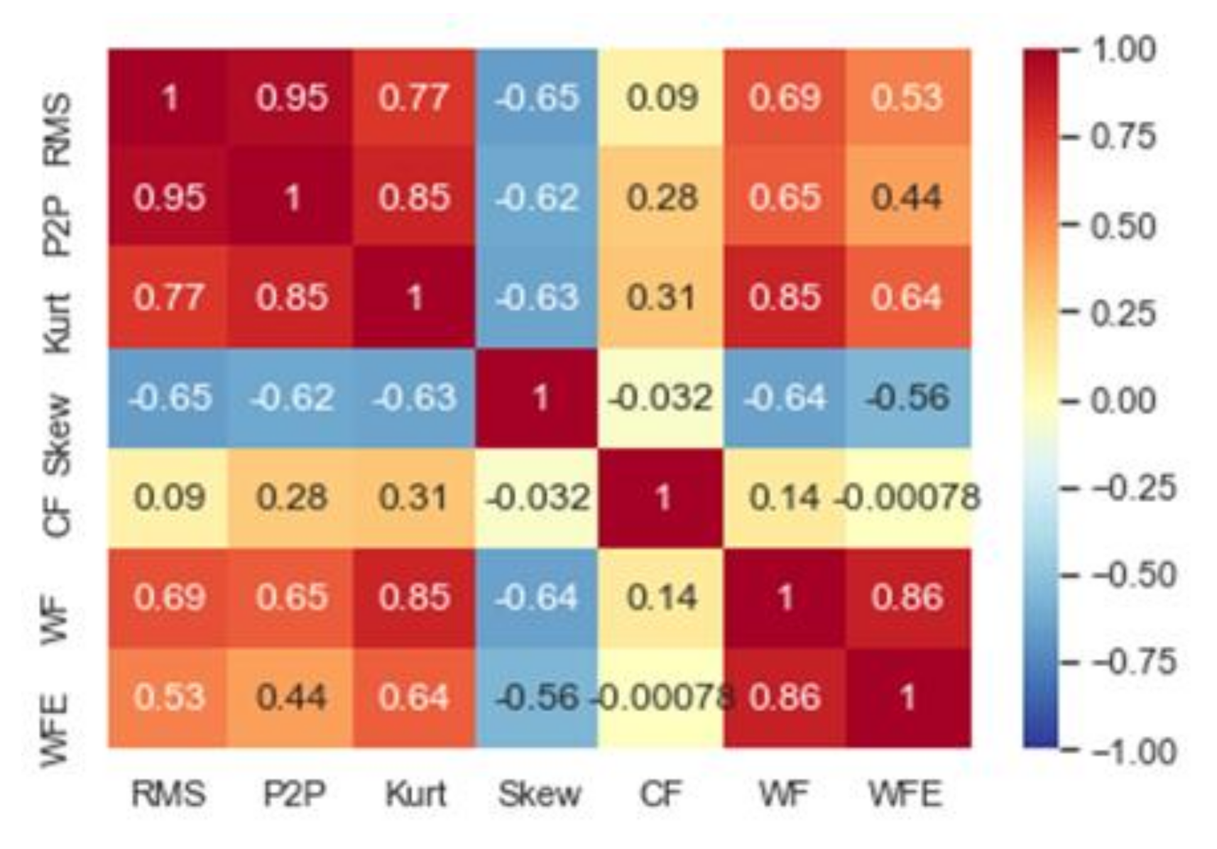
3.2.1. Filtering with Correlation Analysis

In general, various features, such as root mean square (RMS), kurtosis, and skewness, can be used for HIs, representing the state of machinery. However, some of them might have a strong correlation, which means that the effect of one feature can be explained through that of another feature. Due to this characteristic, using features with a strong correlation together may cause overfitting and redundant computation for the derivation of HIs. This so-called multicollinearity is an important issue in various machine learning algorithms, which holds back the performance of the algorithm [34]. Thus, as the first step for selecting significant features, we perform correlation analysis to filter features with a strong correlation. This means that we consider only one of them among strongly correlated features.

For example, if correlation coefficients of features are given as in Figure 4, we can observe that there is a strong correlation between Feature 1 and 2 due to the large value of the correlation coefficient (0.8971). In this case, we can select Feature 1 or Feature 2 as a representative one among those two features. However, we need to consider all possible combinations of features in order to select significant features depending on some performance criteria, such as accuracy.

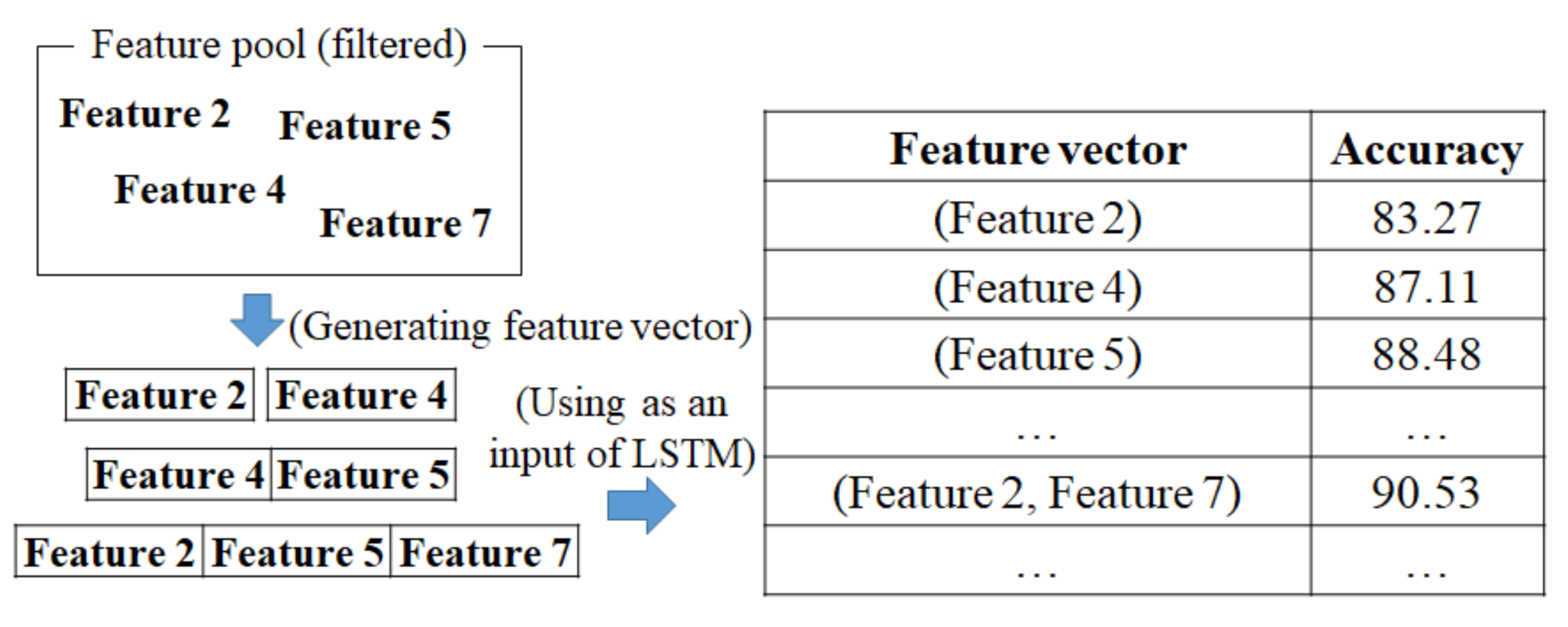
3.2.2. Choosing the Fittest Feature Vector

After filtering significant features by using correlation analysis, we begin considering all possible combinations of remaining features as follows. First, we define feature vectors containing one or more features, which are candidates for HIs. Then, we train a benchmark LSTM model by using the features included in each feature vector as an input to calculate the accuracy of trained LSTM, while setting hyperparameters to specific values. We compare the resulting accuracy values obtained by using feature vectors, and the feature vector with the largest accuracy is selected as the HI. This procedure is described in Figure 5. In this example, Features 2 and 7 are selected as the fittest feature vector. In general, screening is not suitable for feature selection, due to its exhaustive nature. If there exist $m$ features, computational complexity to select the fittest set of features is $O\left(2^m\right)$, which is exponentially proportional to the number of features. However, we carry out correlation analysis to remove surplus features and restrict the maximum length of feature vector to $n$ to avoid the excessive search for feature space. As a result, we can devise a small number of features $m_{small}$ and visit only ${{\displaystyle \sum }}_{i=1}^n{ }_m{C}_i$ feature vectors. This procedure is valid for datasets containing a small number of features or many related features.

3.3. Design of GA for Exploring Optimal Hyperparameters of LSTM

Since hyperparameters related to the structure of LSTM are decided in an integer range, tuning them can be another combinatorial optimization problem. However, there is no efficient pre-processing method, such as correlation analysis performed in Section 3.2.1, which makes hyperparameter tuning more difficult. Additionally, the optimal hyperparameter for a certain dataset cannot guarantee optimality in other datasets. In this work, due to the time step, the number of LSTM layers and hidden neurons in each layer moves in ranges [1, i], [1, j], [1, k], and computation effort is immoderate $O\left(i*j*k\right)$. In addition to identifying a good HI that can be used as a desirable input of LSTM, therefore, we suggest an efficient GA to explore hyperparameters of LSTM that are crucial for the performance of LSTM. The detailed design of the GA is explained in the following subsections.

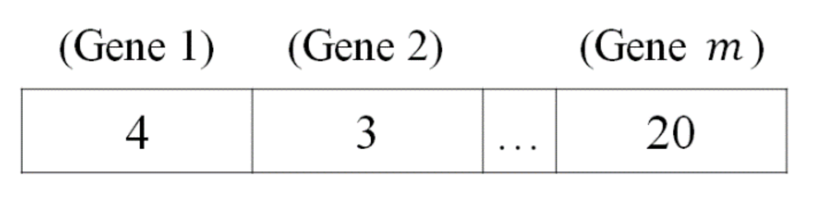
3.3.1. Chromosome Structure and Initial Population

The first step for designing the GA is to devise the representation scheme of the chromosome. Since the objective is to find a set of hyperparameters maximizing the accuracy of trained LSTM, we define a chromosome structure as a vector with integer-valued encoding, where each gene expresses the value of a hyperparameter for trained LSTM. If there exist m hyperparameters to be considered, the length of the chromosome is set to m and the whole structure of the chromosome can be depicted as in Figure 6, where each gene corresponds to each hyperparameter of trained LSTM. For example, in Figure 6, the number 3 in the second gene can represent the number of layers in LSTM. Meanwhile, the population used in the GA contains $P$ chromosomes and an initial population is randomly generated within the lower and upper bounds of hyperparameters, which are defined appropriately.

3.3.2. Fitness Function

A fitness function is used to evaluate whether the chromosome in the population is good or bad, which is important for proper design of the GA. Since we aim to optimize hyperparameters of LSTM, the fitness function should be able to evaluate chromosomes by using the accuracy of trained LSTM with hyperparameters recorded in them. Therefore, we suggest the following fitness function proportional to $Acc$, where $Acc$ means the accuracy and $c$ is a constant.

$$fitness\_function=\frac{1}{c}Acc.$$

(1)

3.3.3. Crossover Operator

The GA investigates the solution space of hyperparameters by an iterative searching process. During this procedure, crossover operator decides the direction and size of moves, which affect the effectiveness and efficiency of the GA. In general, a point crossover is a representative one that simply swaps genes of parental chromosomes according to a randomly selected crossover point. However, this approach cannot generate diverse offspring in the case of integer-valued encoding. As an alternative, we consider an arithmetic crossover operator that generates offspring via an arithmetic operation of values located in the parental chromosomes and preserves the order of genes. Specifically, two gene values, $y_r^1$ and $y_r^2$, corresponding to the $r$-th hyperparameter $\left(r=1,2,\cdots ,m\right)$ in two offspring can be obtained by using $\alpha x_r^1+\left(1-\alpha \right)x_r^2$ and $\left(1-\alpha \right)x_r^1+\alpha x_r^2$, where $x_r^1$ and $x_r^2$ are the $r$-th gene values recorded in the parental chromosomes, and $\alpha$ is a random number generated from [−0.5, 1.5]. However, since these values are real values, we need to modify the equations in order to make them integers by applying a flooring function after adding +0.5 to each of them, as in Equation (2).

$$\begin{gathered} y_r^1=\lfloor \left(\alpha x_r^1+\left(1-\alpha \right)x_r^2\right)+0.5\rfloor \\ {y}_r^2=\lfloor \left(\left(1-\alpha \right)x_r^1+\alpha x_r^2\right)+0.5\rfloor \end{gathered}$$

(2)

3.3.4. Mutation Operator

Similar to mutation occurring in nature, which means the emergence of a feature not observed in the parents, the mutation operator generates a solution containing new features different from those of the parental chromosomes. It prevents the algorithm from converging to a local optimal solution and guarantees the diversity of solutions. We use the Makinen, Periaux, and Toivanen mutation (MPTM) operator that enables a robust search of the solution space specialized in real-valued encoding [35]. If $h{p}_r$ is an original $r$-th hyperparameter, $h{p}_r^{\prime }$ affected by the MPTM operator can be calculated by using the steps depicted in Figure 7, where $U{B}_r$ and $L{B}_r$ are upper and lower bounds that are the same as the ones used in generating the initial population. This operation is performed on the $r$-th gene with the probability of mutation $p_m$.

3.3.5. Updating Population and Termination Criteria of GA

Since there are $P$ chromosomes in the original population and $P$ offspring are generated by crossover and mutation operators, there are a total of $2P$ chromosomes. We choose only $P$ chromosomes with high fitness values in order to maintain the size of the population. Specifically, we apply a roulette wheel selection, which assigns each chromosome with a probability to be chosen as a parental chromosome proportional to its fitness value. Furthermore, we define the termination criteria of the GA by using the number of iterations without improvement. This means that we stop the iteration if no enhancement of the solution is observed after a pre-determined number of iterations. This termination condition can prevent inefficient iterations from providing little improvement of the solution while causing a waste of computational resources [36].

4. A Numerical Experiment

4.1. An Experimental Design

We designed a numerical experiment to evaluate the performance of the solution procedure suggested in this paper as follows. We used a dataset gathered from a repository hosted by NASA. Specifically, we considered the IMS bearing dataset containing vibration sensor data obtained from a performance degradation experiment of four different bearing components of machinery [37]. The bearing is an essential element of machinery which has simple dynamics for analysis and reasonable lifetime for assessment. Each IMS bearing dataset consists of three sets recorded during different timelines with 10 min intervals, which is summarized in

Table 2. Description of three sets belonging to IMS bearing dataset.

Set	Recording Duration	Number of Files	Failure Occurs In
No. 1	10/22/2003 12:06:24 to 11/25/2003 23:39:56	2156	Bearing 3, 4
No. 2	02/12/2004 10:32:39 to 02/19/2004 06:22:39	984	Bearing 1
No. 3	03/04/2004 09:27:46 to 04/04/2004 19:01:57	4448	Bearing 3

. Among them, we utilized the information of Bearing 1 belonging to Set No. 2 to formulate a predictive maintenance model based on LSTM. It contains 984 files generated at each time point recorded over about 7 days.

Each file in the dataset stores 20,480 sensor measurements recorded at one time point. Then, the feature value of a time point was acquired by processing all 984 sensor measurements using a specific equation for calculating the feature value. Figure 8 illustrates an example of the pre-processing of vibration data to calculate the RMS value at all time points, where vibration data recorded at each time point were transformed into the RMS value at that time point. As a result, 984 RMS values were calculated from 984 files included in dataset No. 2.

Including the RMS tackled in the above example, we considered a total of 7 features for processing vibration data at a certain time point as a candidate for the HI [38,39]. Descriptions and equations for calculating each feature are described in

Table 3. Description and equation for calculating features.

Features	Descriptions	Equations for Calculating Features
Root Mean Square (RMS)	Square root of mean square	$RM{S}_t=\sqrt{\frac{1}{N}{{\displaystyle \sum }}_{i=1}^N{x}_i^2}$
Peak-to-Peak	Difference between positive and negative peak	$Pt{P}_t=\max \left(x_i\right)-\min \left(x_i\right)$
Kurtosis	Steepness of distribution of samples	$Kurtosi{s}_t=\frac{\frac{1}{N}{{\displaystyle \sum }}_{i=1}^N{\left(x_i-\overline{x}\right)}^4}{{\left(\frac{1}{N}{{\displaystyle \sum }}_{i=1}^N{\left(x_i-\overline{x}\right)}^2\right)}^2}-3$
Skewness	Asymmetry of distribution of samples	$Skewnes{s}_t=\frac{\frac{1}{N}{{\displaystyle \sum }}_{i=1}^N{\left(x_i-\overline{x}\right)}^3}{{\left(\frac{1}{N}{{\displaystyle \sum }}_{i=1}^N{\left(x_i-\overline{x}\right)}^2\right)}^{3/2}}$
Crest Factor (CF)	Extremeness of positive peak compared to other samples	$C{F}_t=\frac{\max \left(x_i\right)}{\sqrt{\frac{1}{N}{{\displaystyle \sum }}_{i=1}^N{x}_i^2}}$
Waveform Factor (WF)	Coefficient affecting shape of vibration or wave	$W{F}_t=\frac{\sqrt{\frac{1}{N}{{\displaystyle \sum }}_{i=1}^N{x}_i^2}}{\frac{1}{N}{{\displaystyle \sum }}_{i=1}^N\left|x_i\right|}$
Waveform Factor Entropy (WFE)	Entropy of WF to acquire robust values	$WF{E}_t=\frac{1}{M}{\displaystyle {\displaystyle \sum }_{i=0}^{M-1}}W{F}_{t-i}*\log \left(W{F}_{t-i}\right)$

, where $x_i$ is the $i$-th measurement and $\overline{x}$ is the mean of all measurements. Similar to the RMS, each feature was calculated for 984 time slots based on vibration data of 984 files.

The definitions of normal and fault classes used to train the LSTM for detecting fault occurrence were sequences recorded in the time period (300, 450] and (700, 900], respectively, which was the same as the reference model used in [3]. To train the LSTM for monitoring, 70% of sequences belonging to each class were used as a training set, while the rest were used as a test set for validation of the result. Additionally, we committed 100 epochs of training for both LSTMs for prediction and monitoring, with 10 epochs of patience as an early stopping condition, which means that the training procedure may be terminated before 100 epochs if there is no improvement of the performance metric in 10 epochs. Since a desirable input value for neural network is between 0 and 1, we applied 0–1 normalization defined in Equation (3), where $x^{\prime }$ means a normalized value and $x_{min}$ and $x_{max}$ are the minimum and maximum values of the features to be normalized, respectively. The predictive maintenance model was evaluated by the validation accuracy of LSTM for monitoring. All numerical experiments were implemented with Python 3.7 and Spyder IDE.

$$x^{\prime }=\frac{x-x_{min}}{x_{max}-x_{min}}$$

(3)

4.2. Experimental Results

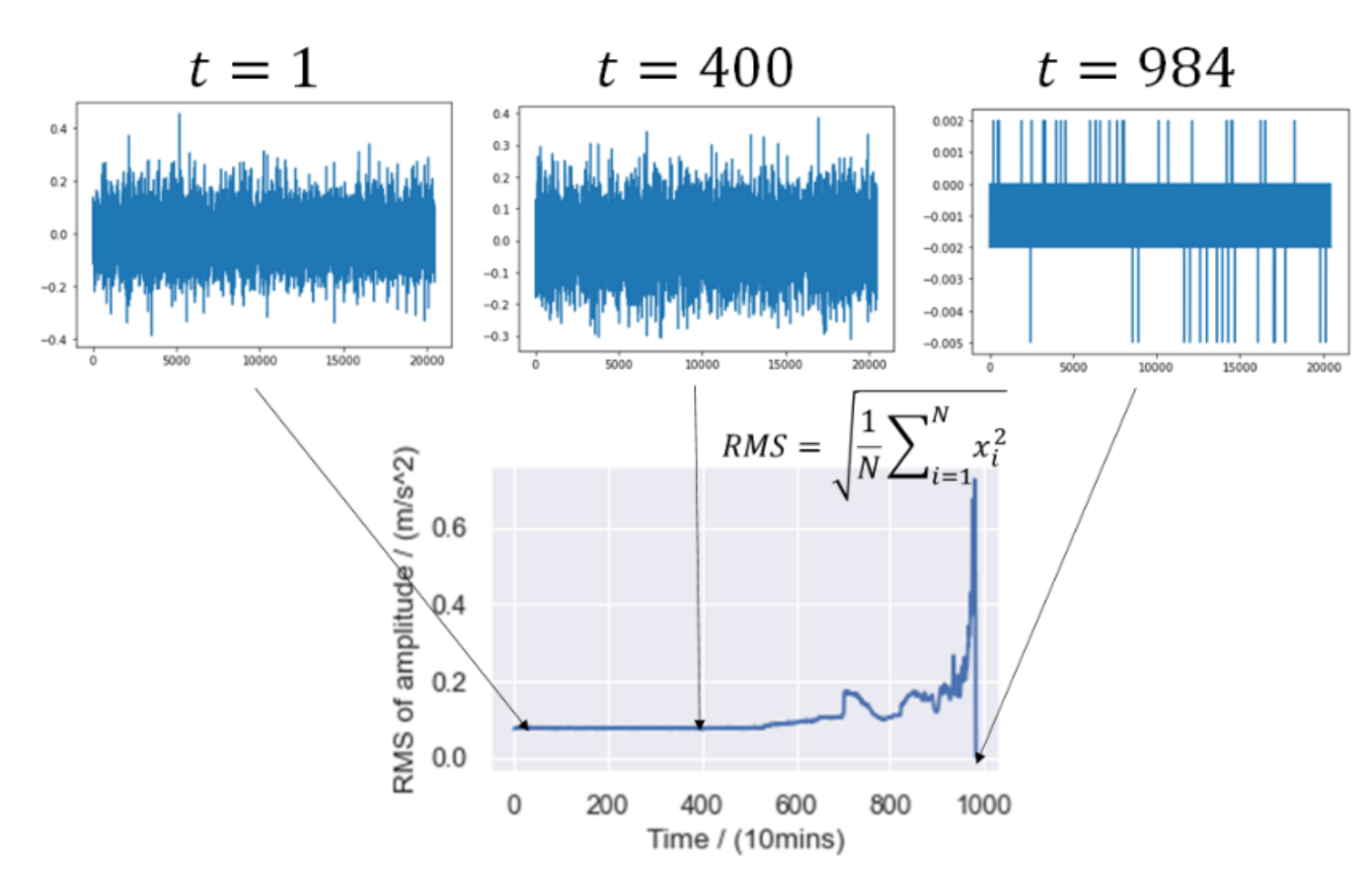
4.2.1. Feature Selection for Defining HI

A correlation matrix of features was computed as in Figure 9. Then, we could apply a filtering operation to select features with strong correlations as follows. We could observe that WF and WFE had a strong correlation coefficient of 0.86 and WF had a strong correlation coefficient of 0.85 with kurtosis. Therefore, we decided to select WFE and kurtosis as representative ones. Furthermore, since RMS, peak-to-peak (P2P) and kurtosis had high correlation coefficients larger than 0.75 and they had similar correlation coefficients with others, we could only consider kurtosis by filtering RMS and peak-to-peak (P2P) out. As a result, we finally selected kurtosis, skewness, crest factor, and waveform entropy as candidates for the HI.

Then, we defined feature vectors containing filtered features and trained the benchmark LSTM using them, where the benchmark LSTM used hyperparameter settings including the number of timesteps = 4, the number of LSTM layers = 3, the number of neurons = 30. The limit of the maximum length of the feature vector was set to 3 for efficient training. We performed 20 repetitions and recorded both the mean and standard deviation of training and validation accuracy calculated from the trained LSTM, which are summarized in

Table 4. Accuracy of trained LSTM by using feature vectors.

Feature Vector	Training Accuracy	Validation Accuracy
	Mean (std. dev.)	Mean (std. dev.)
(Kurtosis)	0.8043 (0.0079)	0.7946 (0.0084)
(Skewness)	0.8188 (0.0078)	0.7950 (0.0098)
(CF)	0.7432 (0.0194)	0.7113 (0.0188)
(WFE)	0.8341 (0.0125)	0.8296 (0.0137)
(Kurtosis, Skewness)	0.8703 (0.0114)	0.8678 (0.0107)
(Kurtosis, CF)	0.8654 (0.0123)	0.8642 (0.0147)
(Kurtosis, WFE)	0.8987 (0.0149)	0.8413 (0.0188)
(Skewness, CF)	0.8422 (0.0144)	0.8063 (0.0164)
(Skewness, WFE)	0.9011 (0.0129)	0.8710 (0.0135)
(CF, WFE)	0.9237 (0.0138)	0.8823 (0.0156)
(Kurtosis, Skewness, CF)	0.9568 (0.0124)	0.9234 (0.0121)
(Kurtosis, Skewness, WFE)	0.9612 (0.0110)	0.9175 (0.0099)
(Kurtosis, CF, WFE)	0.9301 (0.0105)	0.8958 (0.0129)
(Skewness, CF, WFE)	0.8939 (0.0149)	0.8813 (0.0156)

.

We could derive some insights from the experiment as follows. Although WFE showed the best performance among features when they were used alone, a different result appeared when feature vectors containing it were used to train LSTM. Specifically, we could observe that the feature vector with the largest validation accuracy did not include WFE, while the vector contained CF with the lowest validation accuracy among features. A similar tendency appeared in the result of the feature vector with length 3, where feature vectors including kurtosis dominated those including WFE in terms of validation accuracy. Feature vectors with a longer length showed better accuracy in most cases. However, feature vectors with many features brought about additional computation. As a result, we chose the feature vector including kurtosis, skewness, and CF as the HI, which showed the highest validation accuracy.

4.2.2. Exploring Optimal Hyperparameters of LSTM

Using the feature vector obtained in Section 4.2.1, we performed numerical experiments to find the optimal hyperparameter configuration of LSTM by using the GA. A pre-experiment was conducted to set the parameters of the GA, which determined a population size $P=20$ and a probability of mutation $p_m=0.01$. Furthermore, the ranges for time steps, number of LTSM layers, and number of neurons we considered for generating initial population of chromosomes in the GA were [2, 10], [1, 5], [10, 150], respectively. Similar to the experiment executed for feature selection, we considered 20 repetitions and recorded the mean and standard deviation.

Table 5. Comparison of validation accuracy obtained from this research and others.

Referred	Feature	Method	Validation Accuracy
(This paper)	Kurtosis, skewness, crest factor	LSTM with 8 time steps, 3 LSTM layers, 115 hidden neurons	0.9814 (0.099)
Ali et al. [40]	RMS, kurtosis, RMSEE 1	SFAM 2 (3 layers, 6 hidden neurons)	0.7420
Zhang et al. [3]	Kurtosis, waveform factor	LSTM with 8 time steps, 3 LSTM layers, 150 hidden neurons	0.7846
	Kurtosis, waveform factor, waveform entropy	LSTM with 8 time steps, 3 LSTM layers, 150 hidden neurons	0.9312
		Back propagation (BP) network with 3 hidden layers containing 150 hidden neurons	0.7841
		Stacked autoencoder (SAE) with 3 hidden layers containing 150, 100, 50 hidden neurons each	0.8677
		Convolutional neural network (CNN) with 2 convolutional layers (5 × 5 × 32, 5 × 5 × 16) and 2 pooling layers	0.9203
Zhou et al. [41]	RMS, kurtosis, skewness, RMSEE 1, 8 frequency-based features (total 12 features used)	CNN with 5 convolutional layers, 3 pooling layers, and 3 additional fully connected layers except for one before output layer	0.9858
Yu [42]	Seven time-based features (including RMS, kurtosis, skewness, etc.) and 4 frequency and wavelet features (total 11 features)	k-NN with original features	0.9167
		k-NN with features resulting from PCA	0.9167
		k-NN with features resulting from LNPP 3	0.9444
		k-NN with features resulting from LDA 4	0.9722
		k-NN with features resulting from SLNPP 5	0.9722
Roy et al. [43]	Five features (max. value, centroid, abs. centroid, kurtosis, and simple sign integral) among 36 features	Autocorrelation-aided random forest with feature selection and pre-processing including binary classification	0.9790
	Five features (abs. centroid, RMS, impulse factor, 75th percentile, and approximate entropy) among 36 features		0.9824

¹ RMSEE: RMS entropy estimator $\left(\frac{1}{n}{{\displaystyle \sum }}_{i=1}^n-RM{S}_i*log\left(RM{S}_i\right)\right)$. ² SFAM: simplified fuzzy adaptive resonance theory map. ³ LNPP: local and non-local preserving projection-based feature extraction. ⁴ LDA: linear discriminant analysis. ⁵ SLNPP: supervised learning-based LNPP.

displays the experimental results. We included the results of previous research using the same IMS bearing dataset to compare with our work [3,40,41]. Furthermore, we addressed the information of hyperparameters used for each method in order to compare the performance.

Firstly, validation accuracy obtained from this paper had the third highest value among all approaches. The accuracy of LSTM-based approaches dominated other deep learning-based ones such as BP, SAE, and CNN in most cases. This showed the superiority of LSTM for processing vibration data of bearings, which stems from the advantage of LSTM in dealing with time series data. Exceptionally, the CNN considered in [41] slightly outperformed the result of this paper by devising an extremely deep network with a complex trained structure with many features, four times more than those used in this paper. Additionally, they used different proportions of training and test sets, namely 0.8 and 0.2, respectively. Contrary to their work, we defined the compact feature vector used as the HI, maintaining the competitive performance level. Other techniques used for predictive maintenance were also examined to demonstrate the efficiency of our work. For instance, k-nearest neighbor (k-NN) is easy to implement and has a computational advantage. Yu [42] designed elaborate feature selection techniques to improve validation accuracy about 6% from original features. Still, however, our work offers slightly better classification performance represented by validation accuracy. Random forest, a representative machine learning approach, was also considered for predictive maintenance. Roy et al. [43] applied their random forest-based method using two different feature sets, which showed validation accuracy of 0.9790 and 0.9824, respectively. Although the latter shows a slightly more accurate result than our work, it has limitations such that complicated pre-processing is required, and high complexity brings about a lack of scalability which stems from the nature of the decision tree.

Compared to [3], we could observe the following matters. The combination of kurtosis and waveform factor (0.7841) is not desirable, which is worse than using kurtosis alone (0.7946 in Table 4). This tendency might result from multicollinearity between kurtosis and waveform factor, which showed a high correlation coefficient of 0.85 in a previous feature selection experiment. Furthermore, from the comparison of results obtained by feature vectors with the same length, the validation accuracy obtained in this study is higher than that obtained in [3]. In terms of the structure of LSTM, in addition, the number of hidden neurons in each LSTM layer used in this study is smaller than that of [3], which supports that features used as HIs in this paper can express the state of bearing components more elaborately. As a result, desirable levels of hyperparameters could be reached by the GA, based on efficient and effective HI derivation.

5. Conclusions

This paper tackled a predictive maintenance model based on LSTM and its optimization, which is specialized for bearing components of the machinery. Specifically, we (i) established both effective and efficient HIs used to describe the state of bearing components and (ii) devised a GA to explore optimal hyperparameters which determine the internal structure and affect the performance of LSTM. Derivation of the HIs was conducted by correlation analysis to exclude redundant features bringing about multicollinearity and a stepwise comparison of feature vectors including independent features. In addition, we designed a GA to explore optimal hyperparameter configuration of LSTM, which was trained by using HI, kurtosis, skewness, and crest factor, obtained by feature selection. This work can be considered for the following applications. Most of all, useful features for describing the state of machinery can be drawn from raw measurement data and the resulting features can be refined by utilizing the feature selection framework. Additionally, hyperparameter tuning with a GA can be applied to establish general deep learning models as well as those other than LSTM models used for predictive maintenance.

In addition, we suggest the following topics for further research work to be considered. We intend to apply our work to more datasets used for predictive maintenance other than bearing performance data. For instance, a dataset consisting of many features, such as an aerospace turbine engine dataset [44], can benefit from the feature selection scheme of this paper. Additional pre-processing, such as signal processing, which is suitable for predictive maintenance data recorded as raw sensor measurement data, might be another research field. Moreover, we plan to modify internal components of the model by replacing LSTM or the GA with other promising and state-of-the-art network structure or metaheuristic methods.

References

1. GE Oil & Gas. The Impact of Digital on Unplanned Downtime—An Offshore Oil and Gas Perspective. 2016. Available online: https://www.gemeasurement.com/sites/gemc.dev/files/ge_the_impact_of_digital_on_unplanned_downtime_0.pdf (accessed on 14 July 2017).
2. Lei, Y.; Li, N.; Guo, L.; Li, N.; Yan, T.; Lin, J. Machinery health prognostics: A systematic review from data acquisition to RUL prediction. Mech. Syst. Signal Process. 2018, 104, 799–834. [Google Scholar] [CrossRef]
3. Zhang, B.; Zhang, S.; Li, W. Bearing performance degradation assessment using long short-term memory recurrent net-work. Comput. Ind. 2019, 106, 14–29. [Google Scholar] [CrossRef]
4. Baraldi, P.; Mangili, F.; Zio, E. A Kalman Filter-Based Ensemble Approach with Application to Turbine Creep Prognostics. IEEE Trans. Reliab. 2012, 61, 966–977. [Google Scholar] [CrossRef]
5. Paris, P.; Erdogan, F. A Critical Analysis of Crack Propagation Laws. J. Basic Eng. 1963, 85, 528–533. [Google Scholar] [CrossRef]
6. Brighenti, R.; Carpinteri, A.; Corbari, N. Damage mechanics and Paris regime in fatigue life assessment of metals. Int. J. Press. Vessel. Pip. 2013, 104, 57–68. [Google Scholar] [CrossRef]
7. Pais, M.J.; Kim, N.H. Predicting fatigue crack growth under variable amplitude loadings with usage monitoring data. Adv. Mech. Eng. 2015, 7, 1687814015619135. [Google Scholar] [CrossRef]
8. Qian, Y.; Yan, R.; Hu, S. Bearing Degradation Evaluation Using Recurrence Quantification Analysis and Kalman Filter. IEEE Trans. Instrum. Meas. 2014, 63, 2599–2610. [Google Scholar] [CrossRef]
9. Wang, L.; Zhang, L.; Wang, X. Reliability estimation and remaining useful lifetime prediction for bearing based on proportional hazard model. J. Cent. South Univ. 2015, 22, 4625–4633. [Google Scholar] [CrossRef]
10. Nielsen, J.S.; Sørensen, J.D. Bayesian Estimation of Remaining Useful Life for Wind Turbine Blades. Energies 2017, 10, 664. [Google Scholar] [CrossRef] [Green Version]
11. Pei, H.; Hu, C.; Si, X.; Zheng, J.; Zhang, Q.; Zhang, Z.; Pang, Z. Remaining Useful Life Prediction for Nonlinear Degraded Equipment with Bivariate Time Scales. IEEE Access 2019, 7, 165166–165180. [Google Scholar] [CrossRef]
12. Liu, J.; Zio, E. System dynamic reliability assessment and failure prognostics. Reliab. Eng. Syst. Saf. 2017, 160, 21–36. [Google Scholar] [CrossRef] [Green Version]
13. Zhai, Q.; Ye, Z.-S. RUL Prediction of Deteriorating Products Using an Adaptive Wiener Process Model. IEEE Trans. Ind. Inform. 2017, 13, 2911–2921. [Google Scholar] [CrossRef]
14. Loutas, T.; Eleftheroglou, N.; Zarouchas, D. A data-driven probabilistic framework towards the in-situ prognostics of fatigue life of composites based on acoustic emission data. Compos. Struct. 2017, 161, 522–529. [Google Scholar] [CrossRef]
15. Lei, Y.; Li, N.; Gontarz, S.; Lin, J.; Radkowski, S.; Dybała, J. A Model-Based Method for Remaining Useful Life Prediction of Machinery. IEEE Trans. Reliab. 2016, 65, 1314–1326. [Google Scholar] [CrossRef]
16. Marra, D.; Sorrentino, M.; Pianese, C.; Iwanschitz, B. A neural network estimator of Solid Oxide Fuel Cell performance for on-field diagnostics and prognostics applications. J. Power Sources 2013, 241, 320–329. [Google Scholar] [CrossRef]
17. Bossio, J.M.; De Angelo, C.H.; Bossio, G.R. Self-organizing map approach for classification of mechanical and rotor faults on induction motors. Neural Comput. Appl. 2012, 23, 41–51. [Google Scholar] [CrossRef]
18. Ren, L.; Cui, J.; Sun, Y.; Cheng, X. Multi-bearing remaining useful life collaborative prediction: A deep learning approach. J. Manuf. Syst. 2017, 43, 248–256. [Google Scholar] [CrossRef]
19. Zhu, J.; Chen, N.; Peng, W. Estimation of Bearing Remaining Useful Life Based on Multiscale Convolutional Neural Network. IEEE Trans. Ind. Electron. 2019, 66, 3208–3216. [Google Scholar] [CrossRef]
20. Guo, L.; Li, N.; Jia, F.; Lei, Y.; Lin, J. A recurrent neural network based health indicator for remaining useful life prediction of bearings. Neurocomputing 2017, 240, 98–109. [Google Scholar] [CrossRef]
21. Widodo, A.; Yang, B.-S. Machine health prognostics using survival probability and support vector machine. Expert Syst. Appl. 2011, 38, 8430–8437. [Google Scholar] [CrossRef]
22. Khelif, R.; Chebel-Morello, B.; Malinowski, S.; Laajili, E.; Fnaiech, F.; Zerhouni, N. Direct Remaining Useful Life Estimation Based on Support Vector Regression. IEEE Trans. Ind. Electron. 2017, 64, 2276–2285. [Google Scholar] [CrossRef]
23. Chen, C.; Liu, Y.; Wang, S.; Sun, X.; Di Cairano-Gilfedder, C.; Titmus, S.; Syntetos, A.A. Predictive maintenance using cox proportional hazard deep learning. Adv. Eng. Inform. 2020, 44, 101054. [Google Scholar] [CrossRef]
24. Nguyen, T.P.K.; Medjaher, K. A new dynamic predictive maintenance framework using deep learning for failure prognostics. Reliab. Eng. Syst. Saf. 2019, 188, 251–262. [Google Scholar] [CrossRef] [Green Version]
25. Bampoula, X.; Siaterlis, G.; Nikolakis, N.; Alexopoulos, K. A Deep Learning Model for Predictive Maintenance in Cyber-Physical Production Systems Using LSTM Autoencoders. Sensors 2021, 21, 972. [Google Scholar] [CrossRef] [PubMed]
26. Larochelle, H.; Erhan, D.; Courville, A.; Bergstra, J.; Bengio, Y. An Empirical Evaluation of Deep Architectures on Problems with Many Factors of Variation. In Proceedings of the 24th International Conference on Machine Learning, Association for Computing Machinery, New York, NY, USA, 20 June 2007; pp. 473–480. [Google Scholar]
27. Bergstra, J.; Bengio, Y. Random Search for Hyper-Parameter Optimization. J. Mach. Learn. Res. 2012, 13, 281–305. [Google Scholar]
28. Wu, J.; Chen, X.-Y.; Zhang, H.; Xiong, L.-D.; Lei, H.; Deng, S.-H. Hyperparameter Optimization for Machine Learning Models Based on Bayesian Optimizationb. J. Electron. Sci. Technol. 2019, 17, 26–40. [Google Scholar] [CrossRef]
29. Bergstra, J.; Bardenet, R.; Bengio, Y.; Kégl, B. Algorithms for Hyper-Parameter Optimization. In Proceedings of the 24th International Conference on Neural Information Processing Systems, Red Hook, NY, USA, 12 December 2011; Curran Associates Inc.: New York, NY, USA, 2011; pp. 2546–2554. [Google Scholar]
30. Mattioli, F.; Caetano, D.; Cardoso, A.; Naves, E.; Lamounier, E. An Experiment on the Use of Genetic Algorithms for Topology Selection in Deep Learning. J. Electr. Comput. Eng. 2019, 2019, 1–12. [Google Scholar] [CrossRef]
31. Camero, A.; Toutouh, J.; Alba, E. Random error sampling-based recurrent neural network architecture optimization. Eng. Appl. Artif. Intell. 2020, 96, 103946. [Google Scholar] [CrossRef]
32. Yi, H.; Bui, K.-H.N. An Automated Hyperparameter Search-Based Deep Learning Model for Highway Traffic Prediction. IEEE Trans. Intell. Transp. Syst. 2020, 1–10. [Google Scholar] [CrossRef]
33. Victoria, A.H.; Maragatham, G. Automatic tuning of hyperparameters using Bayesian optimization. Evol. Syst. 2021, 12, 217–223. [Google Scholar] [CrossRef]
34. Haitovsky, Y. Multicollinearity in Regression Analysis: Comment. Rev. Econ. Stat. 1969, 51, 486. [Google Scholar] [CrossRef]
35. Mäkinen, R.A.E.; Periaux, J.; Toivanen, J. Multidisciplinary Shape Optimization in Aerodynamics and Electromagnetics Us-ing Genetic Algorithms. Int. J. Numer. Methods Fluids 1999, 30, 149–159. [Google Scholar] [CrossRef]
36. Sivanandam, S.N.; Deepa, S.N. Genetic Algorithm Optimization Problems. In Introduction to Genetic Algorithms; Sivanandam, S.N., Deepa, S.N., Eds.; Springer: Berlin/Heidelberg, Germany, 2008; pp. 165–209. ISBN 978-3-540-73190-0. [Google Scholar]
37. Qiu, H.; Lee, J.; Lin, J.; Yu, G. Wavelet filter-based weak signature detection method and its application on rolling element bearing prognostics. J. Sound Vib. 2006, 289, 1066–1090. [Google Scholar] [CrossRef]
38. Caesarendra, W.; Tjahjowidodo, T. A Review of Feature Extraction Methods in Vibration-Based Condition Monitoring and Its Application for Degradation Trend Estimation of Low-Speed Slew Bearing. Machines 2017, 5, 21. [Google Scholar] [CrossRef]
39. Yiakopoulos, C.; Gryllias, K.; Antoniadis, I. Rolling element bearing fault detection in industrial environments based on a K-means clustering approach. Expert Syst. Appl. 2011, 38, 2888–2911. [Google Scholar] [CrossRef]
40. Ben Ali, J.; Chebel-Morello, B.; Saidi, L.; Malinowski, S.; Fnaiech, F. Accurate bearing remaining useful life prediction based on Weibull distribution and artificial neural network. Mech. Syst. Signal Process. 2015, 56–57, 150–172. [Google Scholar] [CrossRef]
41. Zhou, Q.; Shen, H.; Zhao, J.; Liu, X.; Xiong, X. Degradation State Recognition of Rolling Bearing Based on K-Means and CNN Algorithm. Shock. Vib. 2019, 2019, 1–9. [Google Scholar] [CrossRef]
42. Yu, J. Local and Nonlocal Preserving Projection for Bearing Defect Classification and Performance Assessment. IEEE Trans. Ind. Electron. 2012, 59, 2363–2376. [Google Scholar] [CrossRef]
43. Roy, S.S.; Dey, S.; Chatterjee, S. Autocorrelation Aided Random Forest Classifier-Based Bearing Fault Detection Framework. IEEE Sens. J. 2020, 20, 10792–10800. [Google Scholar] [CrossRef]
44. Saxena, A.; Goebel, K.; Simon, D.; Eklund, N. Damage propagation modeling for aircraft engine run-to-failure simulation. In Proceedings of the 2008 International Conference on Prognostics and Health Management, Denver, CO, USA, 6–9 October 2008. [Google Scholar]
Figure 1. Costs and loss of productivity according to maintenance approaches.
Applsci 11 06450 g001
Figure 2. Used degradation model for HS.
Applsci 11 06450 g002
Figure 3. Suggested procedure for optimizing design parameters.
Applsci 11 06450 g003
Figure 4. An example of correlation matrix between features.
Applsci 11 06450 g004
Figure 5. The procedure for choosing the fittest feature vector.
Applsci 11 06450 g005
Figure 6. Chromosome structure using integer-valued encoding.
Applsci 11 06450 g006
Figure 7. Calculation steps in MPTM operator.
Applsci 11 06450 g007
Figure 8. Pre-processing of vibration data.
Applsci 11 06450 g008
Figure 9. Correlation matrix of features for HI.
Applsci 11 06450 g009