
On the Reliability Assessment of Artificial Neural Networks Running on AI-Oriented MPSoCs


Abstract
:1. Introduction
- We present a methodology to identify the most critical neurons of a neural network by assigning resilience values to each of them. The method bases on two levels of analysis: first, the neuron is viewed as an element of each output class (class-oriented analysis); second, the same is interpreted as belonging to the entire neural network (network-oriented analysis). The method can be efficiently applied to neural networks with any layers and any typologies. The methodology is validated by means of software fault injection (FI) campaigns, using three different convolutional neural networks (CNNs) trained on three different data sets: MNIST, SVHN, and CIFAR-10.
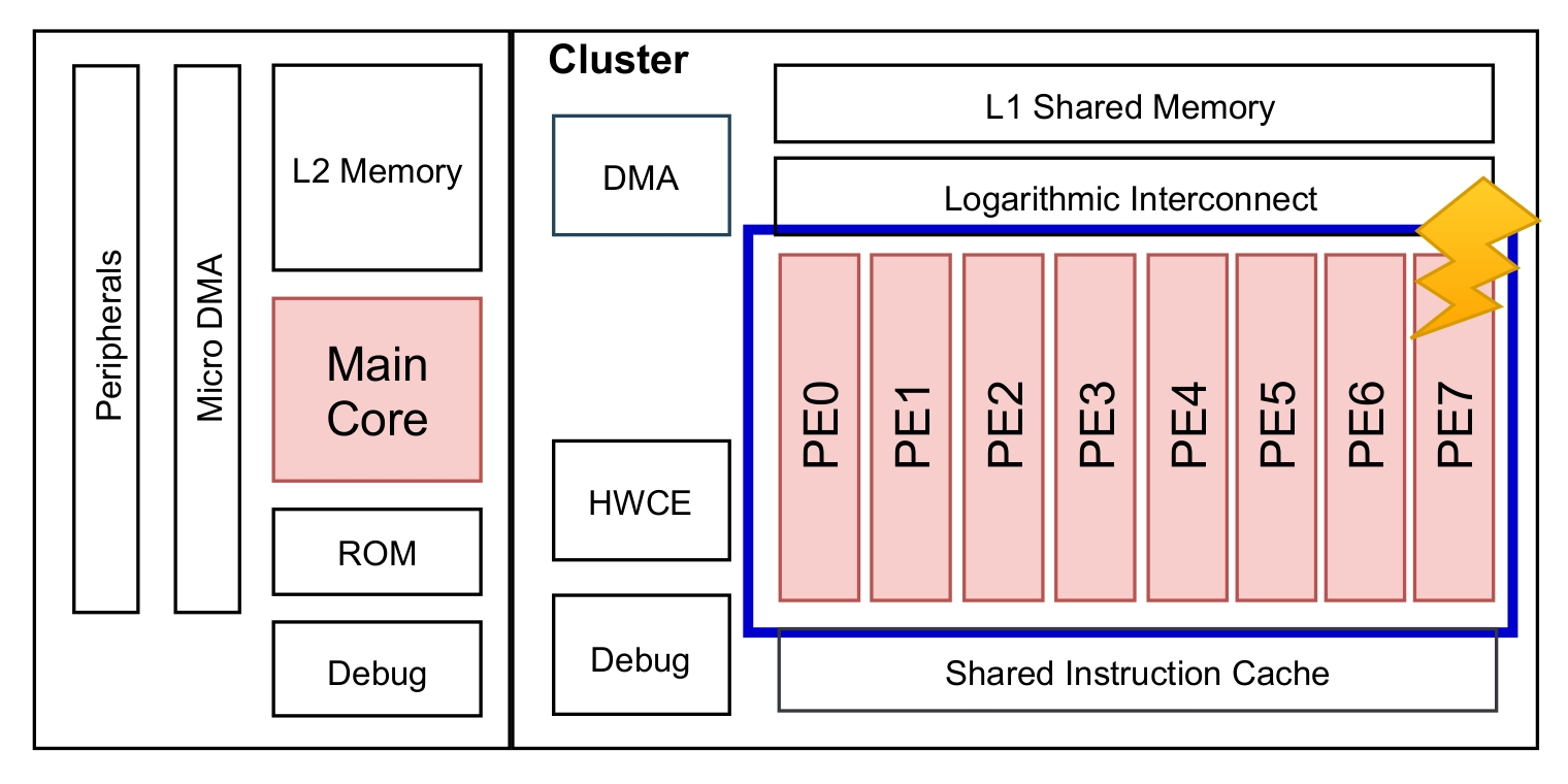
- Based on the above criticality analysis, we describe an approach to evenly distribute critical neurons among the available PEs of the MPSoC to improve the reliability of the NCS. It exploits integer linear programming (ILP) to find the optimal and deterministic solution to map ANNs elaborations onto the target hardware architecture. To prove the effectiveness of this reliability-oriented approach, we carried out FI campaigns at the register transfer level (RTL) on an open-source RISC-V MPSoC for AI at the edge, i.e., the GAP-8 architecture [16]. Specifically, to understand the vulnerability of the MPSoC-based NCS to random hardware faults, permanent faults are addressed in this work. Recent works have highlighted that permanent faults in DNN accelerators have a major impact on DNN accuracy with respect to, for instance, temporary faults (soft errors) [18].
2. Background
2.1. Neural Computing Systems (NCS)
- Behavioral level: It includes the technology independent artificial neural network software model.
- Architectural level: It refers to the hardware exploited for running the ANN model. Examples are graphics processing units (GPUs), field programmable gate arrays (FPGAs), ASICs, and dedicated neurochips.
2.2. Fault Models
- Fault: A fault is an anomalous physical condition or a defect in the system that might occur at the architectural level of a NCS. In order to better study the impact of physical faults in a given device, it is necessary to model them in an accurate way; in the literature, different fault models have been proposed mimicking the fault behavior through a simulable model. Considering their temporal characteristics, physical faults can be mainly classified as permanent or transient. A permanent fault is an unrecoverable defect in the system, such as wires assuming fixed logic values at 0 (stuck-at-0) or 1 (stuck-at-1). Being non-reversible, the fault is stable and fixed over time and affects all the system computations. A transient fault is a defect in the system that is present for a short period of time. It is also known as an intermittent fault or soft error, and it may be due to external perturbations, radiations or disturbances. It is fair to say that today, these two fault models are not able to cover the newer fault mechanisms of the deep-submicrometer technologies: new fault models are needed to deal with delays, stuck-opens, open-lines, bridgings, and transient pulses. A detailed overview is provided in [29]. However, despite the category and the specific fault model, a physical fault may or may not be activated, depending on several factors, such as the input conditions, and thus, may or may not lead to malfunctioning in the application. In the literature, many reliability investigations and studies have been made by exploiting both permanent [30,31] and transient fault models [32,33,34].
- Error: An error, also referred to as behavioral error for exhibiting at the behavioral level, is an unexpected system behavior, for instance, due to the activation of a physical fault. In the neural network field, each neuron is considered a single entity that can fail independently of the failure of any other [5]. Neural networks are viewed as distributed systems consisting of two components: neurons and synapses, i.e., the communication channels connecting the neurons. As for neurons, the error of a synapse is also independent of that of other synapses or neurons. Therefore, we can distinguish between two typologies of errors at the behavioral level:
- Crash: Neurons or synapses completely stop their activity. A crashed synapse can be modeled as a synapse weighted by value 0. Contrarily, to model a crashed neuron, the dropout fault model is exploited, where the output of the neuron is purposely set to 0.
- Byzantine: Neurons or synapses keep their activity but send arbitrary values, within their bounded transmission capacity [35].
An error affecting a single neuron or synapses may not lead to a failure. This is not only related to the intrinsic definition of an error, but also to the ANN property of being over-provisioned. - Failure: A NCS failure occurs when the network, due to the manifestation of errors, wrongly predicts the output. Clearly, it must be underlined that ANNs are usually not 100% accurate: they might wrongly predict the output, even without the occurrence of errors.
2.3. Related Works
3. Proposed Approach
- Ranking of the criticality of single neurons: Resilience scores are assigned to individual neurons of the ANN.
- Mapping and variance assignment: Based on the previous phase and on the available PEs of the target AI-oriented MPSoC, a value is given to each chunk of neurons assigned to a single PE. We adopt a mathematical metric as a decision-making parameter—the variance. This value indicates the criticality of the chunk; in other words, the amount of critical neurons in that chunk that are assigned to a PE.
- ILP-based optimal scheduling: By leveraging on the chunks variance, an ILP solver is set up to obtain the optimal reliability-oriented scheduling for mapping ANN inferences on a specific hardware device.
3.1. Ranking of the Criticality of Single Neurons
- Class-oriented analysis (CoA): For each single output class, the most important neurons are extracted with Algorithm 1 and sorted in descending order based on their criticality. This sorting is saved on a final list, named the score map, which is created for each output class.
- Network-oriented analysis (NoA): The process is repeated for the entire neural network (without distinguishing between output classes), and a single score map is obtained.
- Final network-oriented score-map: The network-oriented score map is updated based on the outcomes of the class-oriented analysis.
| Algorithm 1: Assignment of resilience scores to individual neurons |
 |
3.2. Mapping and Variance Assignment
3.3. ILP-Based Optimal Scheduling
- Each chunk k must be assigned to a single processing element p, multiple assignments of sections of the same layer to a certain machine are not allowed:
- Each processing element p must compute the same amount of chunks k equal to the total amount of layers L:
- Each processing element p in each layer l has to process a single chunk k:
- The cumulative variance elaborated by every PE must be close to the average one:
- The cumulative variance of each layer must stay the same:
4. Case Study
5. Experimental Results
5.1. Ranking of the Criticality of Single Neurons
5.1.1. Class-Oriented Analysis (CoA)
5.1.2. Network-Oriented Analysis (NoA)
5.1.3. Final Network-Oriented Score Map
5.2. Mapping and Optimal Scheduling
- Traditional static scheduling: It is the traditional method where the same range of neurons are assigned always to the same PE, as depicted in Figure 3.
- Proposed ILP and variance-based scheduling: It is the proposed approach described in Section 3.3. It assigns portions of neurons to PEs depending on their criticality.
- SDC-1: A silent data corruption (SDC) failure is a deviation of the network output from the golden network result, leading to a misprediction. Hence, the fault causes the image to be wrongly classified.
- Masked with MSE > 0: The network correctly predicts the result, but the MSE of the faulty output vector is different from zero. It means that the top score is correct but the fault causes a variation in the outputs compared to the fault-free execution.
- Hang: The fault causes the system to hang and the HDL simulation never finishes.
6. Conclusions
Author Contributions
Funding
Institutional Review Board Statement
Informed Consent Statement
Data Availability Statement
Conflicts of Interest
Abbreviations
| AI | Artificial Intelligence |
| ANN | Artificial Neural Network |
| DNN | Deep Neural Network |
| CNN | Convolutional Neural Network |
| ILP | Integer Linear Programming |
| SoC | System-on-a-chip |
| MPSoC | Multiprocessor System-on-a-chip |
| ASIC | Application Specific Integrated Circuit |
| SIMD | Single Instruction Multiple Data |
References
- McCulloch, W.S.; Pitts, W. A logical calculus of the ideas immanent in nervous activity. Bull. Math. Biophys. 1943, 5, 115–133. [Google Scholar] [CrossRef]
- Sejnowski, T.; Delbruck, T. The Language of the Brain; Scientific American Volume 307; Howard Hughes Medical Institute United States: Stevenson Ranch, CA, USA, 2012; pp. 54–59. [Google Scholar] [CrossRef]
- He, K.; Zhang, X.; Ren, S.; Sun, J. Delving Deep into Rectifiers: Surpassing Human-Level Performance on ImageNet Classification. arXiv 2015, arXiv:1502.01852. [Google Scholar]
- Lawrence, S.; Giles, C.; Tsoi, A. What Size Neural Network Gives Optimal Generalization? Convergence Properties of Backpropagation. 2001. Available online: https://drum.lib.umd.edu/handle/1903/809 (accessed on 12 July 2021).
- El Mhamdi, E.M.; Guerraoui, R. When Neurons Fail. In Proceedings of the 2017 IEEE International Parallel and Distributed Processing Symposium (IPDPS), Orlando, FL, USA, 29 May–2 June 2017; pp. 1028–1037. [Google Scholar]
- Kung, H.T.; Leiserson, C.E. Systolic Arrays for (VLSI); Technical Report; Carnegie-Mellon University Pittsburgh Pa Department of Computer Science: Pittsburgh, PA, USA, 1978. [Google Scholar]
- Misra, J.; Saha, I. Artificial neural networks in hardware: A survey of two decades of progress. Neurocomputing 2010, 74, 239–255. [Google Scholar] [CrossRef]
- Palossi, D.; Conti, F.; Benini, L. An Open Source and Open Hardware Deep Learning-Powered Visual Navigation Engine for Autonomous Nano-UAVs. In Proceedings of the 2019 15th International Conference on Distributed Computing in Sensor Systems (DCOSS), Santorini Island, Greece, 29–31 May 2019; pp. 604–611. [Google Scholar] [CrossRef] [Green Version]
- Barkallah, E.; Freulard, J.; Otis, M.J.D.; Ngomo, S.; Ayena, J.C.; Desrosiers, C. Wearable Devices for Classification of Inadequate Posture at Work Using Neural Networks. Sensors 2017, 17, 2003. [Google Scholar] [CrossRef] [PubMed] [Green Version]
- Peluso, V.; Cipolletta, A.; Calimera, A.; Poggi, M.; Tosi, F.; Aleotti, F.; Mattoccia, S. Monocular Depth Perception on Microcontrollers for Edge Applications. IEEE Trans. Circuits Syst. Video Technol. 2021. [Google Scholar] [CrossRef]
- Ottavi, G.; Garofalo, A.; Tagliavini, G.; Conti, F.; Benini, L.; Rossi, D. A Mixed-Precision RISC-V Processor for Extreme-Edge DNN Inference. In Proceedings of the 2020 IEEE Computer Society Annual Symposium on VLSI (ISVLSI), Limassol, Cyprus, 6–8 July 2020; pp. 512–517. [Google Scholar] [CrossRef]
- Wolf, W.; Jerraya, A.A.; Martin, G. Multiprocessor System-on-Chip (MPSoC) Technology. IEEE Trans. Comput. Aided Des. Integr. Circuits Syst. 2008, 27, 1701–1713. [Google Scholar] [CrossRef]
- Ma, Y.; Zhou, J.; Chantem, T.; Dick, R.P.; Wang, S.; Hu, X.S. Online Resource Management for Improving Reliability of Real-Time Systems on “Big–Little” Type MPSoCs. IEEE Trans. Comput. Aided Des. Integr. Circuits Syst. 2020, 39, 88–100. [Google Scholar] [CrossRef]
- Desoli, G.; Chawla, N.; Boesch, T.; Singh, S.P.; Guidetti, E.; De Ambroggi, F.; Majo, T.; Zambotti, P.; Ayodhyawasi, M.; Singh, H.; et al. 14.1 A 2.9TOPS/W Deep Convolutional Neural Network SoC in FD-SOI 28 nm for Intelligent Embedded Systems. In Proceedings of the 2017 IEEE International Solid-State Circuits Conference (ISSCC), San Francisco, CA, USA, 5–9 February 2017; pp. 238–239. [Google Scholar] [CrossRef]
- Sim, J.; Park, J.; Kim, M.; Bae, D.; Choi, Y.; Kim, L. 14.6 A 1.42TOPS/W Deep Convolutional Neural Network Recognition Processor for Intelligent IoE Systems. In Proceedings of the 2016 IEEE International Solid-State Circuits Conference (ISSCC), San Francisco, CA, USA, 31 January–4 February 2016; pp. 264–265. [Google Scholar] [CrossRef]
- Flamand, E.; Rossi, D.; Conti, F.; Loi, I.; Pullini, A.; Rotenberg, F.; Benini, L. GAP-8: A RISC-V SoC for AI at the Edge of the IoT. In Proceedings of the 2018 IEEE 29th International Conference on Application-Specific Systems, Architectures and Processors (ASAP), Milan, Italy, 10–12 July 2018; pp. 1–4. [Google Scholar] [CrossRef]
- Venkataramani, S.; Ranjan, A.; Roy, K.; Raghunathan, A. AxNN: Energy-Efficient Neuromorphic Systems Using Approximate Computing. In Proceedings of the 2014 IEEE/ACM International Symposium on Low Power Electronics and Design (ISLPED), La Jolla, CA, USA, 11–13 August 2014; pp. 27–32. [Google Scholar] [CrossRef]
- Zhang, J.J.; Gu, T.; Basu, K.; Garg, S. Analyzing and Mitigating the Impact of Permanent Faults on a Systolic Array Based Neural Network Accelerator. In Proceedings of the 2018 IEEE 36th VLSI Test Symposium (VTS), San Francisco, CA, USA, 22–25 April 2018; pp. 1–6. [Google Scholar] [CrossRef] [Green Version]
- Bosio, A. Emerging Computing Devices: Challenges and Opportunities for Test and Reliability. In Proceedings of the 26th IEEE European Test Symposium (ETS), Bruges, Belgium, 24–28 May 2021; pp. 1–10. [Google Scholar] [CrossRef]
- Ramacher, U.; Beichter, J.; Bruls, N.; Sicheneder, E. Architecture and VLSI Design of a VLSI Neural Signal Processor. In Proceedings of the 1993 IEEE International Symposium on Circuits and Systems, Chicago, IL, USA, 3–6 May 1993; Volume 3, pp. 1975–1978. [Google Scholar] [CrossRef]
- Cappellone, D.; Di Mascio, S.; Furano, G.; Menicucci, A.; Ottavi, M. On-Board Satellite Telemetry Forecasting with RNN on RISC-V Based Multicore Processor. In Proceedings of the 2020 IEEE International Symposium on Defect and Fault Tolerance in VLSI and Nanotechnology Systems (DFT), Frascati, Italy, 19–21 October 2020; pp. 1–6. [Google Scholar] [CrossRef]
- Cerutti, G.; Andri, R.; Cavigelli, L.; Farella, E.; Magno, M.; Benini, L. Sound Event Detection with Binary Neural Networks on Tightly Power-Constrained IoT Devices. In Proceedings of the ACM/IEEE International Symposium on Low Power Electronics and Design; Association for Computing Machinery: New York, NY, USA, 2020; pp. 19–24. [Google Scholar] [CrossRef]
- Means, R.W.; Lisenbee, L. Extensible Linear Floating Point SIMD Neurocomputer Array Processor. In Proceedings of the IJCNN-91-Seattle International Joint Conference on Neural Networks, Seattle, WA, USA, 8–12 July 1991; Volume 1, pp. 587–592. [Google Scholar] [CrossRef]
- Dai, X.; Yin, H.; Jha, N.K. NeST: A Neural Network Synthesis Tool Based on a Grow-and-Prune Paradigm. IEEE Trans. Comput. 2019, 68, 1487–1497. [Google Scholar] [CrossRef] [Green Version]
- Sung, W.; Shin, S.; Hwang, K. Resiliency of Deep Neural Networks under Quantization. arXiv 2015, arXiv:1511.06488. [Google Scholar]
- Reagen, B.; Gupta, U.; Pentecost, L.; Whatmough, P.; Lee, S.K.; Mulholland, N.; Brooks, D.; Wei, G.Y. Ares: A Framework for Quantifying the Resilience of Deep Neural Networks. In Proceedings of the 55th Annual Design Automation Conference, San Francisco, CA, USA, 24–29 June 2018; Association for Computing Machinery: San Francisco, CA, USA, 2018; pp. 1–6. [Google Scholar] [CrossRef]
- Ruospo, A.; Bosio, A.; Ianne, A.; Sanchez, E. Evaluating Convolutional Neural Networks Reliability depending on their Data Representation. In Proceedings of the 2020 23rd Euromicro Conference on Digital System Design (DSD), Kranj, Slovenia, 26–28 August 2020; pp. 672–679. [Google Scholar] [CrossRef]
- Bushnell, M.; Agrawal, V. Essentials of Electronic Testing for Digital, Memory and Mixed-Signal VLSI Circuits; Springer Publishing Company, Incorporated: Berlin/Heidelberg, Germany, 2013. [Google Scholar]
- Torres-Huitzil, C.; Girau, B. Fault and Error Tolerance in Neural Networks: A Review. IEEE Access 2017, 5, 17322–17341. [Google Scholar] [CrossRef]
- Temam, O. A Defect-Tolerant Accelerator for Emerging High-Performance Applications. In Proceedings of the 2012 39th Annual International Symposium on Computer Architecture (ISCA), Portland, OR, USA, 9–13 June 2012; pp. 356–367. [Google Scholar] [CrossRef]
- Lotfi, A.; Hukerikar, S.; Balasubramanian, K.; Racunas, P.; Saxena, N.; Bramley, R.; Huang, Y. Resiliency of Automotive Object Detection Networks on GPU Architectures. In Proceedings of the 2019 IEEE International Test Conference (ITC), Washington, DC, USA, 9–15 November 2019; pp. 1–9. [Google Scholar] [CrossRef]
- Zhao, B.; Aydin, H.; Zhu, D. Generalized Reliability-Oriented Energy Management for Real-Time Embedded Applications. In Proceedings of the 2011 48th ACM/EDAC/IEEE Design Automation Conference (DAC), San Diego, CA, USA, 5–10 June 2011; pp. 381–386. [Google Scholar]
- Du, B.; Condia, J.E.R.; Reorda, M.S. An Extended Model to Support Detailed GPGPU Reliability Analysis. In Proceedings of the 2019 14th International Conference on Design Technology of Integrated Systems in Nanoscale Era (DTIS), Mykonos, Greece, 16–18 April 2019; pp. 1–6. [Google Scholar] [CrossRef]
- Li, G.; Hari, S.K.S.; Sullivan, M.; Tsai, T.; Pattabiraman, K.; Emer, J.; Keckler, S.W. Understanding Error Propagation in Deep Learning Neural Network (DNN) Accelerators and Applications. In Proceedings of the International Conference for High Performance Computing, Networking, Storage and Analysis; Association for Computing Machinery: New York, NY, USA, 2017. [Google Scholar] [CrossRef]
- Allen, C.; Stevens, C.F. An evaluation of causes for unreliability of synaptic transmission. Proc. Natl. Acad. Sci. USA 1994, 91, 10380–10383. Available online: https://www.pnas.org/content/91/22/10380.full.pdf (accessed on 12 July 2021). [CrossRef] [PubMed] [Green Version]
- He, Y.; Balaprakash, P.; Li, Y. FIdelity: Efficient Resilience Analysis Framework for Deep Learning Accelerators. In Proceedings of the 2020 53rd Annual IEEE/ACM International Symposium on Microarchitecture (MICRO), Athens, Greece, 17–21 October 2020; pp. 270–281. [Google Scholar] [CrossRef]
- dos Santos, F.; Draghetti, L.; Weigel, L.; Carro, L.; Navaux, P.; Rech, P. Evaluation and Mitigation of Soft-Errors in Neural Network-Based Object Detection in Three GPU Architectures. In Proceedings of the 2017 47th Annual IEEE/IFIP International Conference on Dependable Systems and Networks Workshops (DSN-W), Denver, CO, USA, 26–29 June 2017; pp. 169–176. [Google Scholar]
- Luza, L.M.; Söderström, D.; Tsiligiannis, G.; Puchner, H.; Cazzaniga, C.; Sanchez, E.; Bosio, A.; Dilillo, L. Investigating the Impact of Radiation-Induced Soft Errors on the Reliability of Approximate Computing Systems. In Proceedings of the 2020 IEEE International Symposium on Defect and Fault Tolerance in VLSI and Nanotechnology Systems (DFT), Frascati, Italy, 19–21 October 2020; pp. 1–6. [Google Scholar] [CrossRef]
- Bosio, A.; Bernardi, P.; Ruospo, A.; Sanchez, E. A Reliability Analysis of a Deep Neural Network. In Proceedings of the 2019 IEEE Latin American Test Symposium (LATS), Santiago, Chile, 11–13 March 2019; pp. 1–6. [Google Scholar] [CrossRef]
- Neggaz, M.A.; Alouani, I.; Lorenzo, P.R.; Niar, S. A Reliability Study on CNNs for Critical Embedded Systems. In Proceedings of the 2018 IEEE 36th International Conference on Computer Design (ICCD), Orlando, FL, USA, 7–10 October 2018; pp. 476–479. [Google Scholar] [CrossRef]
- Mahmoud, A.; Aggarwal, N.; Nobbe, A.; Vicarte, J.R.S.; Adve, S.V.; Fletcher, C.W.; Frosio, I.; Hari, S.K.S. PyTorchFI: A Runtime Perturbation Tool for DNNs. In Proceedings of the 2020 50th Annual IEEE/IFIP International Conference on Dependable Systems and Networks Workshops (DSN-W), Valencia, Spain, 29 June–2 July 2020; pp. 25–31. [Google Scholar] [CrossRef]
- Ruospo, A.; Balaara, A.; Bosio, A.; Sanchez, E. A Pipelined Multi-Level Fault Injector for Deep Neural Networks. In Proceedings of the 2020 IEEE International Symposium on Defect and Fault Tolerance in VLSI and Nanotechnology Systems (DFT), Frascati, Italy, 19–21 October 2020; pp. 1–6. [Google Scholar] [CrossRef]
- Cun, Y.L.; Denker, J.S.; Solla, S.A. Optimal Brain Damage. In Advances in Neural Information Processing Systems 2; Morgan Kaufmann Publishers Inc.: San Francisco, CA, USA, 1990; pp. 598–605. [Google Scholar]
- Han, S.; Pool, J.; Tran, J.; Dally, W.J. Learning Both Weights and Connections for Efficient Neural Networks. In Proceedings of the 28th International Conference on Neural Information Processing Systems; MIT Press: Cambridge, MA, USA, 2015; Volume 1, pp. 1135–1143. [Google Scholar]
- Wang, J.; Liu, L.; Pan, X. Pruning Algorithm of Convolutional Neural Network Based on Optimal Threshold. In Proceedings of the 2020 5th International Conference on Mathematics and Artificial Intelligence, Chengdu, China, 10–13 April 2020; pp. 50–54. [Google Scholar] [CrossRef]
- Lee, K.; Kim, H.; Lee, H.; Shin, D. Flexible Group-Level Pruning of Deep Neural Networks for On-Device Machine Learning. In Proceedings of the 2020 Design, Automation Test in Europe Conference Exhibition (DATE), Grenoble, France, 9–13 March 2020; pp. 79–84. [Google Scholar] [CrossRef]
- Liu, S.; Wang, X.; Wang, J.; Fu, X.; Zhang, X.; Gao, L.; Zhang, W.; Li, T. Enabling Energy-Efficient and Reliable Neural Network via Neuron-Level Voltage Scaling. In Proceedings of the 2019 IEEE 25th International Conference on Parallel and Distributed Systems (ICPADS), Tianjin, China, 4–6 December 2019; pp. 410–413. [Google Scholar] [CrossRef]
- Schorn, C.; Guntoro, A.; Ascheid, G. Accurate Neuron Resilience Prediction for a Flexible Reliability Management in Neural Network Accelerators. In Proceedings of the 2018 Design, Automation Test in Europe Conference Exhibition (DATE), Dresden, Germany, 19–23 March 2018; pp. 979–984. [Google Scholar] [CrossRef]
- Montavon, G.; Lapuschkin, S.; Binder, A.; Samek, W.; Müller, K.R. Explaining nonlinear classification decisions with deep Taylor decomposition. Pattern Recognit. 2017, 65, 211–222. [Google Scholar] [CrossRef]
- Hanif, M.; Shafique, M. SalvageDNN: Salvaging deep neural network accelerators with permanent faults through saliency-driven fault-aware mapping. Philos. Trans. R. Soc. Math. Phys. Eng. Sci. 2020, 378, 20190164. [Google Scholar] [CrossRef] [Green Version]
- Squire, L.R. Memory systems of the brain: A brief history and current perspective. Neurobiol. Learn. Mem. 2004, 82, 171–177. [Google Scholar] [CrossRef] [PubMed]
- Bosman, T.; Frascaria, D.; Olver, N.; Sitters, R.; Stougie, L. Fixed-Order Scheduling on Parallel Machines. In Integer Programming and Combinatorial Optimization; Lecture Notes in Computer Science (Including Subseries Lecture Notes in Artificial Intelligence and Lecture Notes in Bioinformatics); Nagarajan, V., Lodi, A., Eds.; Springer: Berlin, Germany, 2019; pp. 88–100. [Google Scholar] [CrossRef] [Green Version]
- Shmoys, D.B.; Wein, J.; Williamson, D.P. Scheduling Parallel Machines On-Line. In Proceedings of the 1991 Proceedings 32nd Annual Symposium of Foundations of Computer Science, San Juan, PR, USA, 1–4 October 1991; pp. 131–140. [Google Scholar] [CrossRef]
- Lee, J.H.; Jang, H. Uniform Parallel Machine Scheduling with Dedicated Machines, Job Splitting and Setup Resources. Sustainability 2019, 11, 7137. [Google Scholar] [CrossRef] [Green Version]
- Lecun, Y.; Bottou, L.; Bengio, Y.; Haffner, P. Gradient-based learning applied to document recognition. Proc. IEEE 1998, 86, 2278–2324. [Google Scholar] [CrossRef] [Green Version]
- Netzer, Y.; Wang, T.; Coates, A.; Bissacco, A.; Wu, B.; Ng, A.Y. Reading Digits in Natural Images with Unsupervised Feature Learning. In Proceedings of the NIPS Workshop on Deep Learning and Unsupervised Feature Learning; Curran Associates: Red Hook, NY, USA, 2011. [Google Scholar]
- Krizhevsky, A. Learning Multiple Layers of Features from Tiny Images. Technical Report. 2009. Available online: https://www.cs.toronto.edu/~kriz/learning-features-2009-TR.pdf (accessed on 12 July 2021).
- Paszke, A.; Gross, S.; Massa, F.; Lerer, A.; Bradbury, J.; Chanan, G.; Killeen, T.; Lin, Z.; Gimelshein, N.; Antiga, L.; et al. PyTorch: An Imperative Style, High-Performance Deep Learning Library. In Advances in Neural Information Processing Systems 32; Wallach, H., Larochelle, H., Beygelzimer, A., d’Alché-Buc, F., Fox, E., Garnett, R., Eds.; Curran Associates, Inc.: Red Hook, NY, USA, 2019; pp. 8024–8035. [Google Scholar]
- Sermanet, P.; Chintala, S.; LeCun, Y. Convolutional Neural Networks Applied to House Numbers Digit Classification. In Proceedings of the 21st International Conference on Pattern Recognition (ICPR2012), Tsukuba, Japan, 11–15 November 2012; pp. 3288–3291. [Google Scholar]
- Springenberg, J.T.; Dosovitskiy, A.; Brox, T.; Riedmiller, M. Striving for Simplicity: The All Convolutional Net. arXiv 2015, arXiv:1412.6806. [Google Scholar]
- Garofalo, A.; Rusci, M.; Conti, F.; Rossi, D.; Benini, L. PULP-NN: A Computing Library for Quantized Neural Network inference at the edge on RISC-V Based Parallel Ultra Low Power Clusters. In Proceedings of the 2019 26th IEEE International Conference on Electronics, Circuits and Systems (ICECS), Genoa, Italy, 27–29 November 2019; pp. 33–36. [Google Scholar] [CrossRef]
- Condia, J.E.R.; Reorda, M.S. Testing permanent faults in pipeline registers of GPGPUs: A multi-kernel approach. In Proceedings of the 2019 IEEE 25th International Symposium on On-Line Testing and Robust System Design (IOLTS), Rhodes, Greece, 1–3 July 2019; pp. 97–102. [Google Scholar] [CrossRef]
- Chandra, P.; Singh, Y. Fault Tolerance of Feedforward Artificial Neural Networks-A Framework of Study. In Proceedings of the International Joint Conference on Neural Networks, Portland, OR, USA, 20–24 July 2003; Volume 1, pp. 489–494. [Google Scholar] [CrossRef]
- Org, W.; Mason, A.; Dunning, I. OpenSolver: Open Source Optimisation for Excel. In Proceedings of the Annual Conference of the Operations Research Society of New Zealand, Auckland, New Zealand, 29–30 November 2010. [Google Scholar]


| CNN Model | Data Set | Application | Accuracy | Total Neurons |
|---|---|---|---|---|
| Custom LeNet-5 | MNIST | Image Classification | 99.31 | 48,650 |
| ConvNet | SVHN | Object Recognition | 92.01 | 185,374 |
| All-CNN | CIFAR-10 | Object Recognition | 90.57 | 361,046 |
| Chunks Variance-Static Scheduling | |||||||||
|---|---|---|---|---|---|---|---|---|---|
| Layer | Neurons | PE0 | PE1 | PE2 | PE3 | PE4 | PE5 | PE6 | PE7 |
| L0 | 32,768 | 12 | 10 | 8 | 6 | 5 | 5 | 6 | 4 |
| L1 | 8192 | 31 | 11 | 12 | 11 | 21 | 10 | 18 | 5 |
| L2 | 4096 | 18 | 15 | 17 | 9 | 13 | 8 | 11 | 9 |
| L3 | 1024 | 19 | 7 | 3 | 2 | 5 | 6 | 2 | 3 |
| L4 | 2048 | 1 | 3 | 3 | 4 | 4 | 4 | 4 | 4 |
| L5 | 512 | 1 | 1 | 2 | 2 | 1 | 1 | 2 | 2 |
| L6 | 10 | 1 | 1 | 1 | 1 | 1 | 1 | 1 | 1 |
| Total | 48,650 | 83 | 48 | 46 | 35 | 50 | 35 | 44 | 28 |
| Chunks Variance-Proposed Optimal Scheduling | |||||||||
|---|---|---|---|---|---|---|---|---|---|
| Layer | Neurons | PE0 | PE1 | PE2 | PE3 | PE4 | PE5 | PE6 | PE7 |
| L0 | 32,768 | 8 | 6 | 6 | 4 | 5 | 5 | 12 | 10 |
| L1 | 8192 | 21 | 5 | 10 | 31 | 18 | 12 | 11 | 11 |
| L2 | 4096 | 9 | 9 | 15 | 8 | 13 | 17 | 11 | 18 |
| L3 | 1024 | 3 | 19 | 7 | 2 | 5 | 6 | 3 | 2 |
| L4 | 2048 | 4 | 4 | 3 | 1 | 3 | 4 | 4 | 4 |
| L5 | 512 | 1 | 2 | 1 | 1 | 1 | 2 | 2 | 2 |
| L6 | 10 | 1 | 1 | 1 | 1 | 1 | 1 | 1 | 1 |
| Total | 48,650 | 47 | 46 | 43 | 48 | 46 | 47 | 44 | 48 |
| Fault Injection Results | Static Scheduling | Proposed Scheduling | [%] Variation | ||
|---|---|---|---|---|---|
| Images | [%] | Images | [%] | ||
| SDC-1 | 1338 | 1.63 | 1007 | 1.23 | −24.74 |
| Hang | 71,840 | 87.61 | 65,040 | 79.32 | −9.47 |
| Masked, MSE > 0 | 4910 | 5.99 | 9712 | 11.84 | +97.80 |
| Masked, MSE = 0 | 3912 | 4.77 | 6241 | 7.61 | +59.53 |
| Total | 82,000 | 100 | 82,000 | 100 | |
Publisher’s Note: MDPI stays neutral with regard to jurisdictional claims in published maps and institutional affiliations. |
© 2021 by the authors. Licensee MDPI, Basel, Switzerland. This article is an open access article distributed under the terms and conditions of the Creative Commons Attribution (CC BY) license (https://creativecommons.org/licenses/by/4.0/).
Share and Cite
Ruospo, A.; Sanchez, E. On the Reliability Assessment of Artificial Neural Networks Running on AI-Oriented MPSoCs. Appl. Sci. 2021, 11, 6455. https://doi.org/10.3390/app11146455
Ruospo A, Sanchez E. On the Reliability Assessment of Artificial Neural Networks Running on AI-Oriented MPSoCs. Applied Sciences. 2021; 11(14):6455. https://doi.org/10.3390/app11146455
Chicago/Turabian StyleRuospo, Annachiara, and Ernesto Sanchez. 2021. "On the Reliability Assessment of Artificial Neural Networks Running on AI-Oriented MPSoCs" Applied Sciences 11, no. 14: 6455. https://doi.org/10.3390/app11146455
APA StyleRuospo, A., & Sanchez, E. (2021). On the Reliability Assessment of Artificial Neural Networks Running on AI-Oriented MPSoCs. Applied Sciences, 11(14), 6455. https://doi.org/10.3390/app11146455