Article

On the Reliability Assessment of Artificial Neural Networks Running on AI-Oriented MPSoCs

Dipartimento di Automatica e Informatica (DAUIN), Politecnico di Torino, 10129 Turin, Italy
*
Author to whom correspondence should be addressed.
Appl. Sci. 2021, 11(14), 6455; https://doi.org/10.3390/app11146455
Submission received: 11 June 2021 / Revised: 8 July 2021 / Accepted: 9 July 2021 / Published: 13 July 2021

Abstract

:
Nowadays, the usage of electronic devices running artificial neural networks (ANNs)-based applications is spreading in our everyday life. Due to their outstanding computational capabilities, ANNs have become appealing solutions for safety-critical systems as well. Frequently, they are considered intrinsically robust and fault tolerant for being brain-inspired and redundant computing models. However, when ANNs are deployed on resource-constrained hardware devices, single physical faults may compromise the activity of multiple neurons. Therefore, it is crucial to assess the reliability of the entire neural computing system, including both the software and the hardware components. This article systematically addresses reliability concerns for ANNs running on multiprocessor system-on-a-chips (MPSoCs). It presents a methodology to assign resilience scores to individual neurons and, based on that, schedule the workload of an ANN on the target MPSoC so that critical neurons are neatly distributed among the available processing elements. This reliability-oriented methodology exploits an integer linear programming solver to find the optimal solution. Experimental results are given for three different convolutional neural networks trained on MNIST, SVHN, and CIFAR-10. We carried out a comprehensive assessment on an open-source artificial intelligence-based RISC-V MPSoC. The results show the reliability improvements of the proposed methodology against the traditional scheduling.

1. Introduction

In recent years, to face the growing complexity of emerging computing systems and algorithms, artificial intelligence (AI)-based solutions and, specifically, brain-inspired computing models have gained large interest in both industry and academia. Particularly, researchers have developed artificial models named artificial neural networks (ANNs) by imitating biological neurons and their functioning in the human brain. Since their origin [1], a huge number of studies have made progress in improving the theory behind brain-inspired computations to build highly complex artificial models, such as deep neural networks (DNNs). The human brain is a complex and fascinating system able to bear synapse or neuron faults and still keep working properly, thanks to its plastic ability to remodel, repair, and reorganize its neural functions [2]. Today, ANNs are considered attractive solutions, for example, in tasks such as image classification performed in safety-critical applications, such as self-driving cars, radars, flight control, robots, and space applications, due to their outstanding computational capabilities as well as their proven human-level performance [3].
However, to use them safely in human contexts, there is a compelling need for assessing their reliability and tolerance to faults.
Frequently, ANNs are considered inherently fault tolerant and tightly robust, brain-inspired models. This is motivated by two principal reasons: the first is related to their distributed and parallel structure; the second to the redundancy introduced because of over-provisioning [4]. As a matter of fact, ANNs are furnished with a quantity of neurons higher that the minimal number required to perform a computation. It means that they can bear a bounded number of errors thanks to the excessive neuron budget: once this number is exceeded, the precision degrades gracefully as the number of errors increases [5].
Nevertheless, we advocate that the theory claiming the intrinsic ANNs fault tolerance may hold true only in two cases: if neural networks are merely viewed as a software and a mathematical abstraction; if there is a one-to-one correspondence between the neurons and the hardware processing elements (PEs) on which the ANN model runs. This mapping is typical for systolic array structures, the first examples of digital architectures devised for ANNs dating back to 1978 [6]. Although most of the existing ANN applications are developed as software, there are specific models that demand real-time and parallel processing capabilities. Dedicated ANN hardware implementations offer benefits in terms of speed, power, and cost. However, not all hardware architectures are based on systolic array structures, tearing down the theory claiming the ANNs’ inherent reliability. Since their inception, several silicon implementations of neural networks have been proposed in the literature [7]. Particularly worthy of note is the emerging trend toward the development of custom hardware implementations of neural networks, which are extremely fast and ultra-low-power, optimized for solving specific tasks. Examples are ANNs deployed on resource-constrained application-specific integrated circuits (ASICs), such as miniaturized robots (e.g., drones) [8], or even on pervasive embedded systems, such as wearable devices and medical decision-making instruments [9]. Moreover, to face data confidentiality issues and bandwidth limitations, a recent trend is to push deep learning computations from the cloud into the edge [10,11], such as Internet-of-Things (IoTs) devices running deep learning applications. Clearly, this requires the adoption of embedded devices, which are low-power and low-cost on the one side, and powered for computationally intensive calculations on the other. To meet all these requirements, multiprocessor systems-on-a-chip (MPSoCs) currently represent the best option for running AI-based applications [12,13]. They are heterogeneous SoCs made of multiple CPUs and/or multiple PEs along with other hardware subsystems, such as specific hardware accelerators [14,15,16].
The combination of the hardware architecture with the ANN software model in this work is referred to as a Neural Computing System (NCS). From the reliability point of view, it must be said that, due to the size and the resultant complexity of current ANNs, a single PE is not connected to a single neuronal computation (as for systolic architectures) in the state-of-the-art architectures. It would be unfeasible to develop a system with thousands or millions of PEs. It also means that a single physical fault affecting a PE might compromise the activity of multiple neurons.
Therefore, if neural networks can withstand a limited number of killed neurons without compromising their performance [5], understanding the connections between the neurons and the available hardware PEs is essential to trace a comprehensive reliability assessment of the NCS. With respect to the limited number of killed neurons that an ANN can withstand, it is worth underlying that individual network parts differ in their error resilience [17]. Particularly, neurons exhibit different fault tolerance and resilience levels. Some of them strongly contribute to the output classification of the neural network, and their failures have a greater influence on the degradation of the final predictions. All of these considerations justify the claim that neural networks running on hardware designs cannot be considered inherently fault tolerant without investigating the entire system’s reliability.
Motivated by the above-mentioned considerations, the intent of the article is many-fold. The first goal is to tackle the reliability aspect of neural networks with the aim of demonstrating that they are not generally intrinsically resilient; their reliability must be evaluated with respect to the intended hardware implementation. In this regard, the second goal of the article is to propose a methodology to improve the reliability of NCSs based on resource-constrained MPSoCs. The main contributions of this paper are listed in the following:
  • We present a methodology to identify the most critical neurons of a neural network by assigning resilience values to each of them. The method bases on two levels of analysis: first, the neuron is viewed as an element of each output class (class-oriented analysis); second, the same is interpreted as belonging to the entire neural network (network-oriented analysis). The method can be efficiently applied to neural networks with any layers and any typologies. The methodology is validated by means of software fault injection (FI) campaigns, using three different convolutional neural networks (CNNs) trained on three different data sets: MNIST, SVHN, and CIFAR-10.
  • Based on the above criticality analysis, we describe an approach to evenly distribute critical neurons among the available PEs of the MPSoC to improve the reliability of the NCS. It exploits integer linear programming (ILP) to find the optimal and deterministic solution to map ANNs elaborations onto the target hardware architecture. To prove the effectiveness of this reliability-oriented approach, we carried out FI campaigns at the register transfer level (RTL) on an open-source RISC-V MPSoC for AI at the edge, i.e., the GAP-8 architecture [16]. Specifically, to understand the vulnerability of the MPSoC-based NCS to random hardware faults, permanent faults are addressed in this work. Recent works have highlighted that permanent faults in DNN accelerators have a major impact on DNN accuracy with respect to, for instance, temporary faults (soft errors) [18].
In this paper, it will be experimentally proven that, without recurring to retraining or redundancy techniques, it is possible to mitigate the effects of hardware faults by redistributing the neural computations. Indeed, conventional mitigation techniques that are based on redundancy do not fit well with the compute-intensive nature of neural networks, introducing huge overheads [19].
The rest of the paper is organized as follows. Section 2 provides the reader with background knowledge on neural computing systems with a relevant focus on MPSoC-based ones. In the same section, fault models and some of the most relevant works in the literature are presented. Section 3 describes the proposed approach, and Section 4 outlines the case study. Next, Section 5 reports on the experimental results. Finally, Section 6 draws some conclusions and future directions.

2. Background

This section introduces background knowledge on the topics dealt with throughout the article. Initially, Section 2.1 presents the concept of neural computing systems with a special emphasis on AI-oriented MPSoCs. Then, to assist the reliability analysis, the most-used fault models for NCS reliability analysis are described in Section 2.2. Finally, Section 2.3 gives an overview on the related works in the literature.

2.1. Neural Computing Systems (NCS)

A neural computing system is a system that includes the neural network software together with the target architectural implementation. It can be considered a unique block comprising two non-independent levels:
  • Behavioral level: It includes the technology independent artificial neural network software model.
  • Architectural level: It refers to the hardware exploited for running the ANN model. Examples are graphics processing units (GPUs), field programmable gate arrays (FPGAs), ASICs, and dedicated neurochips.
As stated before, the choice of the architectural implementation plays a crucial role in the assessment of the NCS reliability. A survey on all major design approaches and models is proposed in [7], where the main architectural solutions for NCSs are described, including digital, analog, hybrid, FPGA-based, RAM-based, and neuromorphic implementations. Systolic array structures are the first examples of digital architectures devised for ANNs [20]. Their design is suited to express the recurrence and parallelism associated with neural networks. Considering multilayered back-propagation networks, the singular processing element implements the function of an associated neuron, while the weights are stored in a circular memory. It means that a fault in a neuron can be mapped to a single physical fault, e.g., stuck-at fault or transient fault. In this particular scenario, a single physical fault corresponds to a single error in the neuron.
Traditionally, ANNs are executed on programmable high-performance GPUs. However, despite their excellent achievements, they are unsuitable for applications requiring low-cost and, particularly, low-power devices, due to the excessive power consumption for an inference task. For this class of applications, ASICs are gaining growing interest. A growing number of NCSs, especially those intended for the IoT field and for the edge computing paradigms, are built on ASIC design implementations [21,22]. One essential reason is attributed to their flexibility, which makes them suitable for a wide range of applications requiring low-power and low-cost embedded devices. Additionally, modern architectures of digital devices, especially those destined for the AI world, require the parallelization of many computational units, due to the high computational demand. Hence, they mostly exploit the data parallelism with the single-instruction multiple-data (SIMD) computing paradigm, where the parallelism is achieved by applying a single instruction to multiple data items. This means that each PE elaborates the same instructions simultaneously but on different data [23]. In this regard, a PE may correspond either to a processor core [16] or a sub-unit including only the multiplier, the accumulator and an on-chip memory for weights storage. It is worth saying that one of the main issues regarding ASIC-based NCSs is the limited storage capacity. Their on-board memories are suited to host network parameters, i.e., weights, biases. However, being resource-constrained devices, they can hold a limited amount of data, approximately from a few kilobytes [16] up to, in the best case, megabytes [14]. This restriction implies that only bounded-sized ANNs can run inferences on top of resource-constrained embedded devices. In this light, compression algorithms are proposed, such as in [24], where a synthesis tool is presented to compact ANNs architectures during training. Furthermore, researchers have introduced novel quantization models to face this issue [25]. It has been experimentally demonstrated that, moving from a full precision representation (i.e., floating-point) to optimized models exploiting reduced bit-width data types (i.e., fixed-point), the accuracy loss is negligible and the memory footprint can be reduced [26,27]. In this work, we refer to AI-oriented MPSoC to define a class of ASIC digital devices sharing all these features and conceived for running ANNs [14,15,16].

2.2. Fault Models

In the literature, a well established cause–effect relationship exists between three aspects: faults–errors–failures [28]. Depending on the abstraction level and on the fault location, the following classification is drawn:
  • Fault: A fault is an anomalous physical condition or a defect in the system that might occur at the architectural level of a NCS. In order to better study the impact of physical faults in a given device, it is necessary to model them in an accurate way; in the literature, different fault models have been proposed mimicking the fault behavior through a simulable model. Considering their temporal characteristics, physical faults can be mainly classified as permanent or transient. A permanent fault is an unrecoverable defect in the system, such as wires assuming fixed logic values at 0 (stuck-at-0) or 1 (stuck-at-1). Being non-reversible, the fault is stable and fixed over time and affects all the system computations. A transient fault is a defect in the system that is present for a short period of time. It is also known as an intermittent fault or soft error, and it may be due to external perturbations, radiations or disturbances. It is fair to say that today, these two fault models are not able to cover the newer fault mechanisms of the deep-submicrometer technologies: new fault models are needed to deal with delays, stuck-opens, open-lines, bridgings, and transient pulses. A detailed overview is provided in [29]. However, despite the category and the specific fault model, a physical fault may or may not be activated, depending on several factors, such as the input conditions, and thus, may or may not lead to malfunctioning in the application. In the literature, many reliability investigations and studies have been made by exploiting both permanent [30,31] and transient fault models [32,33,34].
  • Error: An error, also referred to as behavioral error for exhibiting at the behavioral level, is an unexpected system behavior, for instance, due to the activation of a physical fault. In the neural network field, each neuron is considered a single entity that can fail independently of the failure of any other [5]. Neural networks are viewed as distributed systems consisting of two components: neurons and synapses, i.e., the communication channels connecting the neurons. As for neurons, the error of a synapse is also independent of that of other synapses or neurons. Therefore, we can distinguish between two typologies of errors at the behavioral level:
    • Crash: Neurons or synapses completely stop their activity. A crashed synapse can be modeled as a synapse weighted by value 0. Contrarily, to model a crashed neuron, the dropout fault model is exploited, where the output of the neuron is purposely set to 0.
    • Byzantine: Neurons or synapses keep their activity but send arbitrary values, within their bounded transmission capacity [35].
    An error affecting a single neuron or synapses may not lead to a failure. This is not only related to the intrinsic definition of an error, but also to the ANN property of being over-provisioned.
  • Failure: A NCS failure occurs when the network, due to the manifestation of errors, wrongly predicts the output. Clearly, it must be underlined that ANNs are usually not 100% accurate: they might wrongly predict the output, even without the occurrence of errors.
It is worth pointing out that understanding the direct connections between single physical faults and crashed/byzantine neurons is an open challenge today. An attempt was recently made by He et al. in [36], where a framework was developed to study the behavior of hardware transient errors in deep learning accelerators. The framework, named Fidelity, is able to model transient faults in software with high fidelity, only leveraging on high-level design information obtained from architectural descriptions. By relying on these hardware-level faults derived from the architectural analysis, they injected random bit-flips at specific input values, weights, and output neurons of the neural network under assessment.
To sum up, the fault models explored in this work are permanent faults at the architectural level, crash errors (precisely, dropout) at the behavioral level, and failures at the application output.

2.3. Related Works

Recent studies have demonstrated that hardware faults induced by an external perturbation or due to silicon wearout and aging effects can significantly impact the DNN inference, leading to prediction failures [29,37,38]. Many attempts have been made in recent years to understand the reliability and the fault tolerance of ANNs [27,34,39,40]. Among the existing techniques, fault injections have been intensively used to assess the dependability of the systems under test: the procedure consists of introducing faults/errors into the system and checking its behavior in response to them. Moreover, to perform fault injection campaigns, many frameworks have been proposed at different abstraction levels and by following specific injection procedures (e.g., [26,41,42]).
Among the existing topics, understanding the importance of individual neurons took on great relevance when the problem of complex ANN models running on limited computing and memory resources emerged. To tackle such problems, many researchers provided network pruning techniques to remove either redundant neurons or connections from over-parameterized neural models. The first pruning algorithm was proposed by LeCun in the 1990s [43], causing many researchers to spend a lot of effort in the network compression field. In [44], a three-step method is described to cut redundant connections by learning the important ones and retraining the remaining sparse network. Without any loss of accuracy, they can reduce the number of connections by 9 to 13 times. A second paper provides an algorithm to remove neurons whose importance is below an optimal threshold [45]. To understand if neurons or connections can be removed, it is a common approach to use tuned thresholds or explore machine learning approaches [46], albeit rarer. Although our problem may seem to be a pruning related one, it departs from it. Our scope is not to compress the network by removing unimportant neurons or connections. Rather, our scope is to find where the most important neurons are and to profile the application criticality. This will drive the subsequent ILP optimal scheduling. Most importantly, contrary to pruning approaches, the methodology presented in this work does not require additional learning steps or the adoption of a threshold, which are computationally expensive.
The importance of neurons in a neural network is also addressed by Venkataramani et al. [17] to design energy-efficient hardware implementations of large-scale neural networks. To characterize the importance and the resilience of each neuron, the backpropagation of error gradients is used to discover those neurons that impact output quality the least. Neurons that contribute the least to the global error are more resilient and can be approximated with energy-efficient neurons. The process implies that, for each input in the training set, the error at the output is computed using forward propagation. Then, the errors are backpropagated to the outputs of individual neurons to get their average error contribution over all inputs in the training set. Finally, the errors are ordered based on the magnitude of their average error contribution. On this base, the same methodology is exploited by Liu et al. in [47] to determine the fault tolerance capability of each neuron, albeit for a different scope. This measure, named δ i , for the i-th neuron is computed as the derivative of the cost function E with respect to the output node yi. A low δ i corresponds to a more resilient neuron, and vice-versa.
δ i = E y i
We see two principal problems with the two above-mentioned techniques ([17,47]). The first one is related to computational costs: to compute the average error contribution (the neuron measure of resilience), it is required to perform both the forward propagation and backpropagation for each instance of the training set. In the proposed approach, only forward propagation is applied for each instance of the training set. Second, the derivative of the cost function implies that the golden output must be available; in other words, the training set must be labeled. This means that the method can be used only with supervised learning neural networks.
A further contribution in this direction is given by Schorn et al. in [48], where the authors propose a methodology to assign resilience values to individual neurons. It is based on the deep Taylor decomposition of neural networks described in [49], which computes the contribution of each neuron to the output function value of a neural network. For each input image, the Taylor decomposition and layerwise relevance propagation (LRP) algorithm computes the value Ri,j for each neuron j belonging to the layer i, as described in [48]. This rule is used with the intent of calculating the average contribution of each neuron (with a score between 0 and 1) over a set of M training images. In more details, based on the training set, the resilience score r of each neuron yi,j is computed as follows:
r i , j = M m = 1 M 1 R i , j ( y 0 , m , t m )
where t is the output label vector related to the input image y0. Similar to [17,47], this methodology requires the output labels to be available, and thus, it restricts the applicability of the technique to neural networks that are trained with a supervised learning procedure. Additionally concerning the computational cost, the backpropagation phase must be repeated twice: first to compute the contribution of each neuron to the output function value with the Taylor decomposition and LRP (Ri,j); next, to compute the contribution of each neuron to the output function value ri,j.
Although the above-mentioned problems can be considered to be of relative importance, it is possible to highlight that all these approaches can be classified as network-oriented: they do not consider the importance of neurons as entities linked to the single output classes. As described in the following, in Section 3, neurons that are critical for individual output classes may take a low resilience score in network-oriented approaches. In this work, we propose to strengthen the network-oriented analysis with a class-oriented one to improve the accuracy of the process that must provide an order set of important neurons, helping, in this way, to improve the reliability level of the system under assessment. To the best of our knowledge, this is the first time that the importance of neurons as related to the single output class is taken into account. However, since this stands in close relation to our research and they pursue a very analogous objective to ours, we compare our approach with a similar method ([48]) later in Section 5.
Finally, as for the proposed reliability-oriented ILP-based methodology, a similar work was recently proposed by Hanif et al. in [50]. The authors described SalvageDNN, a fault-aware mapping methodology that permutes neurons and weights in a DNN such that the least critical weights are mapped to faulty PEs. In this way, they are bypassed by fault aware pruning (FAP) without impacting the accuracy of the DNN. Despite the interesting results, we differ from [50] in the way we assign criticality scores. While Hanif et al. considered only the static parameters (i.e., weights, bias, filters), in our work, we consider also the contribution of the inputs (dynamic approach).
The above analyses have mostly motivated the following proposed methodology.

3. Proposed Approach

The proposed methodology is based on the identification of the most critical neurons inside the ANN to then determine the best scheduling of the ANN application workload in the targeted MPSoC. We assume that the ANN is ready to be deployed on the intended hardware architecture and any modifications of the ANN application are not required. Indeed, only the pretrained ANN application and the available hardware resources are considered. As experimentally demonstrated, the proposed technique is capable of increasing the reliability of the NCS. In this work, we present a methodology that is built on the following three steps:
  • Ranking of the criticality of single neurons: Resilience scores are assigned to individual neurons of the ANN.
  • Mapping and variance assignment: Based on the previous phase and on the available PEs of the target AI-oriented MPSoC, a value is given to each chunk of neurons assigned to a single PE. We adopt a mathematical metric as a decision-making parameter—the variance. This value indicates the criticality of the chunk; in other words, the amount of critical neurons in that chunk that are assigned to a PE.
  • ILP-based optimal scheduling: By leveraging on the chunks variance, an ILP solver is set up to obtain the optimal reliability-oriented scheduling for mapping ANN inferences on a specific hardware device.
These three phases are shown in Figure 1 and detailed in the following.

3.1. Ranking of the Criticality of Single Neurons

If a neuron contributes more to the final prediction, it is considered critical or important; otherwise, it is considered resilient or redundant. An error in critical neurons may significantly compromise the accuracy of the final neural network prediction. From another perspective, determining the most critical neurons of a neural network means identifying all those neurons carrying more information than others. The investigation of ANNs as mathematical models induced us to reflect that a neuron’s output is nothing but the result of a summation. Based on the above insight, we demonstrate that critical neurons are those producing at their output the highest absolute values during the inferences. Moreover, our theoretical-based criticality analysis is founded on a further key observation. According to behavioral theories in neuroscience [51], brain memories occur when specific groups of neurons are reactivated. Based on precise stimuli, neurons become active in a particular pattern of neuronal activity. It means that if our brain thinks of a sky or a meadow, different ensembles of neurons become active. By transferring this concept to the world of artificial neural networks, in a multi-output neural network, the contribution of a single neuron can be seen in two ways. One is meant for guaranteeing the correct prediction of the single output class, and the other is meant for guaranteeing the correct predictions of the entire multi-output neural network. In other words, imagine you have a two-output neural network classifying apples and pears pictures; there will be neurons that are more significant for the class apple and others for the class pear. At the same time, all the neurons guarantee overall correct predictions. To this end, we propose a methodology to assign resilience scores to individual neurons. It is built in three steps:
  • Class-oriented analysis (CoA): For each single output class, the most important neurons are extracted with Algorithm 1 and sorted in descending order based on their criticality. This sorting is saved on a final list, named the score map, which is created for each output class.
  • Network-oriented analysis (NoA): The process is repeated for the entire neural network (without distinguishing between output classes), and a single score map is obtained.
  • Final network-oriented score-map: The network-oriented score map is updated based on the outcomes of the class-oriented analysis.
These three phases are carefully described in the following.
In the first class-oriented analysis, we consider the importance of a neuron related to each single output class. In particular, it is worth specifying that we refer to the neuron as the following: each pixel in the output feature maps of a convolutional layer, each node in the pooling (min, max, average) or fully connected layers. Typically, batch normalization and activation functions (e.g., rectified linear unit, sigmoid, Gaussian) are not considered independent layers, and thus, they do not come with additional neurons. In Algorithm 1, scores are assigned to neurons considering both static and dynamic parameters of the ANN: by catching the neuron’s output (y), both the weights (static parameters) and the inputs (dynamic parameters) are taken. At the beginning, an initial score equal to zero is assigned to each neuron (line 6). Therefore, for each output class of the neural network (line 7), a new score map is created (line 8). For each instance in the training data set related to the specific output class, a forward propagation cycle is performed (line 10). In the meantime, a score is given to each neuron (lines 13–15), by averaging the absolute output values produced during all the inferences (line 20). The score is updated at every inference iteration. At the end of the process, each class keeps its own score map, where every neuron holds a score value (line 22). The highest absolute scores are relative to the most critical neurons for that given class. In more detail, the score map is represented as a list sorting the neurons from the highest to the lowest value. It is worth noting that the output is sampled for every neuron after the eventual batch normalization or activation function.
Algorithm 1: Assignment of resilience scores to individual neurons
Applsci 11 06455 i001
Starting from the classes’ score maps, it is possible to extract a subset (t) of critical neurons in the form className_critical_t. The subset parameter (t) determines the amount of neurons that are considered critical and it is not a fixed value. Defining that number means tuning the reliability of a NCS: in other words, the larger the size, the larger the set of neurons that are considered critical.
Next, in the network-oriented analysis (NoA) phase, we build a final score map where neurons are sorted based on the magnitude of their average contribution over the training set, without differentiating between the output classes. It is worth pointing out that both the score maps resulting from the NoA and the one from the CoA contain all the neurons of the neural network: only their values change, and consequently the ordering. To this end, Algorithm 1 is run again: line 7 is removed and line 9 is modified so that the inputs are picked up from the entire training data set. Then, since it might happen that the neurons that were found to be critical for individual classes take on a low value in the NoA, the outcome of this score map is updated considering the score maps resulting from the CoA. All neurons assuming a higher value in the class-oriented score map (given a subset parameter t) are overwritten. The set of critical neurons to take into account for the final network-oriented score map is computed by executing the union without repetitions of all the classes’ score maps (C), as follows:
c r i t i c a l _ t i = 1 C c i _ c r i t i c a l _ t
As an example, the whole process is illustrated in Figure 2 for a generic neural network trained on MNIST. First, a percentage of critical neurons is selected (t) from the class-oriented score maps. Among these neurons, all those with a lower value in the network-oriented score map are overwritten with the highest value in the classes, i.e., the red squares, whereas neurons, such as Neuron 27 in Class 0, having a value lower in the t % of the CoA, are not updated in the final score map. Interestingly, Neuron 653 in Class 9 assumes the lowest value in the network-oriented score map and, being part of the t%, is updated. In the end, as depicted in the right side of Figure 2, the final updated network-oriented score map is produced, where the per-class criticality is considered with a t factor. The larger t is, the more neurons are considered critical and therefore, strengthened in the final network-oriented score map.
In Section 2.3, similar approaches developed to identify the network’s critical neurons are described. As stated before, they are based only on a network-oriented analysis [17,47,48]. In this paper, we demonstrate that our methodology obtains a stronger analysis in terms of reliability. Although this approach is applied on an ANN performing image classification, it can also be extended to other tasks.

3.2. Mapping and Variance Assignment

In state-of-the-art architectures, a DNN inference task is scheduled, using the one-to-many paradigm (one PE elaborates many neuronal computations). To optimize the memory accesses and to ease the inference process, a typical approach is to assign each PE always the same range of neurons throughout the network inference. Such an approach, named static scheduling, doubtlessly leads to gains in terms of performance and latency, but turns out to be disadvantageous from the reliability point of view. Indeed, a single physical fault affecting a PE insists always on the same range of neurons, no matter their importance.
Traditionally, to improve parallelism, AI-oriented MPSoCs distribute the ANN workload, exploiting the SIMD paradigm. As shown in Figure 3, the neurons N = {0, ..., n} are neatly distributed among all the P = {0, ..., p} PEs, and it is known exactly which neurons that a PE handles when launching the inference of a L-layer neural network, where L = {0, ..., l}. Thus, it is possible to split the total amount of neurons in well-defined chunks, consisting of fixed groups of neurons assigned, at each layer l, to a specific PE p. Nevertheless, the amount of critical neurons belonging to each chunkl,p is not equally distributed among the P computing resources. From the reliability point of view, this might open serious concerns. According to the motivation of the work, a physical fault affecting the architectural level may negatively affect the computation of many neurons at the behavioral level. In addition, most interestingly, what happens if a physical fault hits the PE that processes the greatest number of critical neurons? The hypothesis is that it will emphasize even more the errors, leading to a significant drop in accuracy.
In this work, we provide a way of balancing the assignment of the chunksl,p to the P processing elements, thereby reducing the likelihood that a physical fault on a PE may jeopardize the correct functionality of a large number of critical neurons. In more detail, this study proposes a scheduling mechanism to allocate the chunks of neurons to the available PEs. Since we are not considering any retraining of the ANN, the trend of neurons cannot change. The only way is to redistribute their allocation to the available PEs so that the computation of the most critical neurons is not assigned to just one PE, or a subset of them.
To measure the criticality of a group of neurons (also referred to as chunk), we use the variance parameter. Seeing that it measures how far a data set is spread out, the variance of a chunk of neurons can provide a measure of the number of critical ones contained in that chunk. Mathematically, it is defined as the average of the squared differences from the mean μ . In the beginning, the variance figure for each chunk is computed, with the aim of evaluating their criticality. Given subset of neurons xi,i∈[1,N] assigned to a PEp,p∈[1,P], the variance of the chunkl,p can be computed as described in (4). N represents the total number of neurons in the chunk. A large variance figure suggests that a significant number of critical neurons are enclosed in that chunk. In contrast, a small variance value indicates that the chunk holds a small number of critical neurons.
σ 2 l , p = i = 1 N ( x i μ ) 2 N

3.3. ILP-Based Optimal Scheduling

We propose an ILP and variance-based scheduling with the aim of mitigating the ANN criticality by redistributing chunks of neurons over the existing PEs. An ILP model is built to feed a solver in charge of finding the optimal solution. The final optimized scheduling is deterministic and it is wholly decided at compile-time. Therefore, no choices are made at run-time during the network inference.
The following method takes inspiration from the existing scheduling on parallel machines [52,53,54], where a set of identical machines M = {1, ..., m} has to process in parallel a set of jobs J = {1, ..., j}. Jobs can be split into multiple sections that can be processed on several machines simultaneously, and each job jJ has weight wj and processing time ptj. In line with this, we may consider the machines mM as the processing elements pP of our NCS and the jobs jJ as the layers lL of our ANN. From this point on, the terms machines and processing elements as well as jobs and layers are equivalent, i.e., m = p and j = l. Hence, the problem looks very similar but we change the criterion adopted to find the optimal solution. Indeed, depending on the criteria defining the problem, an optimal scheduling solution can be provided by exploiting, for example, integer linear programming. For instance, if the goal is to to minimize the maximum completion time of machines, scheduling provides a solution for that purpose by assigning those jobs jJ to the machines mM. Although our problem is approaching very closely, our purpose is not to minimize the maximum completion time of machines; rather, it is to equalize the amount of critical neurons that each PE has to elaborate. Therefore, instead of considering the weights wj or the processing time ptj, the criterion on which our scheduling is built is the variance σ 2 j , m of the job’s sections (i.e., the chunks), that measures their criticality (4). In other words, the objective of the proposed method is to uniform the variance of the jobs over the machines.
An optimal and deterministic solution for this problem can be obtained by resorting to optimization solvers. More formally, our approach formulates the problem as an ILP problem, which can be expressed through mathematical formulas. We built an ILP model by defining the decision variables, the objective function, and the constraints, all compliant with the following formulas. The optimal solution is the one that is able to minimize the distance between the machines’ cumulative variance and the average one.
Let us make the following definitions, assuming that 1 ≤ lL and 1 ≤ pP, where L is the total number of layers and P is the total number of available PEs. Then, we need to introduce a third index 1 ≤ kK that refers to the order of the chunks. Such a parameter indicates also how many chunks can be obtained by distributing the workload of layer l over the available PEs (if P is equal to 8, then K will correspond to 8). In static scheduling, the index k is always equal to p: for instance, the chunk1 is always assigned to PE1. With the proposed ILP and variance-based mapping, we change this order and so we need to differentiate between p and k.
As decision variables, integer variables x(l,p)k are used to indicate whether the chunk k of the layer l is assigned to the processing element p or not.
Specifically, x(l,p)k is a binary variable and is equal to the following:
x ( l , p ) k = 1 if   chunk   k   of   layer   l   is   assigned   to   processing   element   p ; 0 otherwise .
The variance of the chunk k of the layer l is fixed ( σ 2 ( l , p ) k ), regardless of the PE to which it is associated. Hence, we can avoid the index p and only refer to σ 2 ( l , k ) .
The objective function of our ILP problem is the following:
Minimize k = 1 K l = 1 L p = 1 P σ 2 ( l , k ) x ( l , p ) k
This is subject to the following constraints:
  • Each chunk k must be assigned to a single processing element p, multiple assignments of sections of the same layer to a certain machine are not allowed:
    p = 1 P ( x ( l , p ) k ) = 1 , l L , k K
  • Each processing element p must compute the same amount of chunks k equal to the total amount of layers L:
    l = 1 L k = 1 K ( x ( l , p ) k ) = L , p P
  • Each processing element p in each layer l has to process a single chunk k:
    k = 1 K ( x ( l , p ) k ) = 1 , l L , p P
  • The cumulative variance elaborated by every PE must be close to the average one:
    k = 1 K l = 1 L ( σ 2 ( l , k ) x ( l , p ) k ) p = 1 P σ 2 p ( T O T ) P , l L
  • The cumulative variance of each layer must stay the same:
    k = 1 K p = 1 P ( σ 2 ( l , k ) x ( l , p ) k ) = σ 2 l ( T O T ) , l L

4. Case Study

To prove the effectiveness of the proposed methodology, we used three different convolutional neural networks (CNNs) trained on three representative and popular data sets: MNIST [55], SVHN [56], and CIFAR-10 [57]. The MNIST data set is used to recognize handwritten digits and consists of a training set of 60,000 28 × 28 gray-scale images, and a test set of 10,000 examples. The street view house numbers (SVHN) data set is a real-world image data set obtained from house numbers in Google Street View images. It contains more than 600,000 digit images: 73,257 digits are used for training, 26,032 digits for testing, and additional ones as extra training data. SVHN comes in two formats: the original and 32 × 32 cropped. We used the latter. The CIFAR-10 data set is an object recognition data set made of 60,000 32 × 32 color images comprising 50,000 training images and 10,000 test images [57].
We implemented three CNNs, using PyTorch [58] on a Linux server equipped with a dual Intel Xeon CPU E5-2680 v3 and 256 GB of RAM. PyTorch is a fast and flexible framework widely used by both industry and academia for deep learning and machine learning based applications. The first neural network is a custom version of LeNet-5 and is composed of 7 layers (i.e., 3 convolutional, each one followed by max pooling and the last fully connected) with an input size of 28 × 28 × 1. After each convolutional layer, the rectified linear (ReLU) activation function was used. It was trained and tested on the MNIST data set reaching a 99.31% of accuracy over the MNIST test set. Next, we implemented a second neural network following the ConvNet [59] model. It was trained and tested over SVHN dataset, classifying correctly the 92.01% of test images. It consists of 2 convolutional layers, each one followed by LP-pooling and normalization layers (also known as 2-stages or multistage features). They were fed to a 2-layer classifier (fully connected layers). The last CNN was built with the all-CNN configuration [60], an architecture that consists solely of convolutional layers ([60] demonstrates that max-pooling can simply be replaced by a convolutional layer with increased stride without loss in accuracy). The architecture is made of 9 convolutional layers. We exploited the CIFAR-10 data set for this last CNN. The final accuracy was equal to 90.57% over the test set. Further details, such as the total amount of neurons, are provided in Table 1.
Furthermore, to demonstrate the effectiveness of the proposed ILP-based scheduling, we carried out fault injections at RTL on a NCS, comprising the custom LeNet CNN (Table 1), running on an open-source AI-oriented RISC-V MPSoC. This ASIC platform is the PULP cluster of RISC-V based processors, named GAP-8 [16]. It comprises two separate domains. The principal one consists of an advanced microcontroller unit, called the fabric controller. It is built around a main RISC-V core, which is intended to handle the SoC principal functionalities. This is aided by a second domain, i.e., a cluster of eight RISC-V cores used by the main core for offloading highly computational-intensive SIMD operations. Hereinafter, the 8 RISC-V cores are named PEs and represent our target hardware elements. Regarding the cluster, the eight cores are identical and are allowed to run the same binary code on different data (SIMD paradigm). The MPSoC hosts in the fabric controller a 512 kB of L2 memory and a ROM storing the primary boot code. In the cluster, each core can access a shared L1 memory. The DMA unit is in charge of handling the transfers between the L2 and the L1 memories. Specifically, a complete CNN inference cycle (a single prediction) takes 276,529 clock cycles (15,772 ms at 18 MHz). Initially, the network parameters (weights, biases) are stored in the 512 KB L2 memory; before each layer computation, the DMA is in charge of transferring the current layer parameters from L2 memory to the cluster’s shared 128 KB L1 memory. Further architectural details are provided in [16]. Moreover, the RISC-V cores of GAP-8 do not have a hardware floating-point unit, and all computations are executed in fixed-point arithmetic. Therefore, the targeted LeNet CNN was quantized to comply with the PULP-NN library requirements [61] and to fit into PULP memories. Unfortunately, due to memory constraints, full-precision neural networks cannot be easily ported into resource-constrained devices, as stated in Section 2. Then, the CNN parameters were quantized to 8-bit signed integers. Specifically, the full-precision PyTorch model’s parameters (weights and biases) were quantized, and then a new model running on the multiprocessor SoC was created in the C programming language by exploiting the kernel functions of PULP-NN. The accuracy of the new quantized network was computed by running the MNIST test set, and it slightly decreased by 1.1%. The reader should note that the final network-oriented score map did not change after the quantization step.

5. Experimental Results

In this section, the experimental analysis and corresponding results are provided along with accurate discussions. First, we performed the analysis of critical neurons for the three CNNs described as case study (Section 5.1). Then, to demonstrate the effectiveness of the proposed scheduling, we executed FI campaigns at the architectural level on the RTL design of the open-source PULP platform running the custom LeNet CNN. All the experiments were performed on a Linux server equipped with a dual Intel Xeon CPU E5-2680 v3 and 256 GB of RAM. The experimental results are provided in Section 5.2.

5.1. Ranking of the Criticality of Single Neurons

To profile the criticality of the three CNNs, Algorithm 1 was executed to assign resilience scores to individual neurons. As stated before, the MNIST, SVHN, and CIFAR-10 training data sets were used to assign resilience scores. In contrast, their test data sets were used for the fault injections experiments (both at the software and RTL level).

5.1.1. Class-Oriented Analysis (CoA)

Initially, each training data set was divided into subclasses, i.e., the number of outputs. More specifically, in our case study, we had ten outputs for all CNNs, but the same reasoning applies to a different number of output classes. Each sub-class contained only the images representing the selected output class. Hence, the proposed algorithm was executed to obtain the ten final score maps for each CNN. Each of them ordered the total neurons from the one activated with the highest average value to the one with the lowest (from the most critical to the least one) for that particular output class.
Next, we performed software FI campaigns (i) to shed light on the importance of the class-oriented analysis, and (ii) to show that individual output classes hold different robustness levels with respect to errors. This certainly depends on the training phase and the structure of the data set that is used to train the network (typically, in the training set, training images are not evenly distributed among the output classes). We exploited the dropout probability fault model (p-dropout) in which a fraction of the neurons outputs is set to zero, and thus, their contribution is canceled. The same fixed amount of neuron outputs (p) was set to zero in two scenarios and, after the injection, the resulting accuracy of each CNN was measured by running the total test set of images (which was different from the training set used to gather the resilience scores). For each output class, in the first scenario (Random), neurons were randomly chosen from the class score map. In the second (Critical), the same number of neurons was neatly selected always starting from the top of the class score map, i.e., from the most critical neurons. As for the Random scenario, since we relied on a random choice of neurons to kill, the experiments were repeated 1000 times (every time picking up different p random neurons); we report in Figure 4, Figure 5 and Figure 6 the average percentage obtained through the experiments. The experiments were conducted for each output class of the targeted CNNs and, particularly, they were replicated for growing p-percentages: p equal to 0.1% (Figure 4a, Figure 5a and Figure 6a); p equal to 0.5% (Figure 4b, Figure 5b and Figure 6b); p equal to 1% (Figure 4c, Figure 5c and Figure 6c); p equal to 1.5% (Figure 4d, Figure 5d and Figure 6d).
The experimental results for the three FI campaigns are reported in Figure 4, Figure 5 and Figure 6. The scenario Fault-free is the golden accuracy of the class and, as for the Random and Critical scenarios, it was computed by running only the inferences of the images belonging to the given output class. As shown, it is evident that random injections do not affect, or only to a negligible extent (when p gets bigger), the behavior of the neural network. Indeed, in all cases, the accuracy fluctuates around the Fault-free one, apart from the third and fourth cases (p = 1% and p = 1.5%) where it slightly decreases. This confirms the theory under which neural networks are equipped with more neurons than they need [4]. In fact, up to a certain point, they can obtain enough of some neurons and still work correctly. On the other hand, this is not confirmed in the Critical scenario. The accuracy of the output classes considerably drops when killing the p highest neurons.
Concerning MNIST LeNet, for p = 0.1% (Figure 4a), the maximum percentage variation from the Fault-free accuracy to scenario Critical is equal to 6.13% and corresponds to the last class (digit 9). Then, when killing p = 0.5% critical neurons (Figure 4b), the highest percentage variation drastically increases, reaching 44.33% for the second class (digit 1), where the CNN accuracy drops from Fault-free 99.33% to 54.54%.
The situation worsens with p = 1% for all the classes, except for digits 5 and 7, where the accuracy keeps close to 60% (Figure 4c). In the last scenario, when dropping p = 1.5% critical neurons from the classes, the correct predictions become zero or close to it. As illustrated in Figure 4d, it turns out that for LeNet trained on MNIST data set, the most robust class corresponds to digit 5, while the least robust is digit 4.
The outcome of the software fault injection for the SVHN network (ConvNet) is shown in Figure 5. When crashing p = 0.1% Critical neurons, the CNN accuracy decreases until reaching a maximum percentage variation equal to 7.3% for digit 9 (Figure 5a). With the increase in the dropped critical neurons p = 0.5%, we observe a considerable drop in accuracy, with a maximum of 61.9% of variation percentage still for digit 9 (Figure 5b). The correct functionality of the neural network worsens considerably for p = 1% until it reaches zero in almost all classes for p = 1.5% (Figure 5c,d). Overall, the most robust class turns out to be the third one, i.e., digit 2. In fact, despite the dropped neurons, it is able to keep an accuracy close to 80% with the highest neurons dropped of 927 (p = 0.5%). On the other hand, the least resilient class is the last one (digit 9). In fact, it is significantly sensitive to removed neurons (starting from p = 0.1%).
With respect to LeNet (MNIST) and ConvNet (SVHN), All-CNN (CIFAR-10) demonstrates greater sensitivity. As shown in Figure 6a, we can observe a greater reduction in accuracy from p = 0.1% (the maximum drop in accuracy is for Class “Horse” and corresponds to 16.2% from the Fault-free value). In addition, for p = 0.5%, all the classes’ accuracy stays under 60%, with the maximum variation percentage from the golden accuracy equal to 69.82% for the class “Horse” (Figure 6b). When the dropped neurons become p = 1% from each class (meaning about 1854 neurons over the total 185,374), the accuracy of the classes drops below 20%, except for the class “Car” with 21.4% (Figure 6c). The experimental results indicate that the most robust class is the class “Car”, while the least resilient one is class “Horse” (Figure 6d).
Overall, data from Figure 4, Figure 5 and Figure 6 suggest similar conclusions, and the different per-class resilience is confirmed in the three targeted CNNs. It is clear that the p-percentage refers to different CNNs of different sizes: the CIFAR-10 network contains almost 7.54× and 4× the number of neurons than the MNIST and SVHN networks, respectively. It means that the former starts misbehaving with about 361 neurons crashed (p = 0.1%), while the other two (with the same percentage) with about 49 and 185, respectively. Finally, these outcomes experimentally demonstrate the initial assumption stating that there are neurons playing a key role, and therefore, are defined critical for the output classes.
To avoid confusion, we used the p parameter to indicate the amount of neurons dropped from the individual classes, and the t parameter to represent the set of critical neurons in the network-oriented score map. They are both percentages working on the score maps, but the first is used in the class-oriented analysis and is used to drop neurons, while the second in used in the network-oriented analysis and serves as a parameter to indicate the reliability level of the system.

5.1.2. Network-Oriented Analysis (NoA)

So far, we have performed software FI campaigns to demonstrate that each output class owns a set of neurons that are more important than others for correctly predicting their images. If this is considered when ranking the network’s neurons based on their criticality, we experimentally demonstrate that the reliability analysis becomes more accurate. In this phase, we computed the neurons’ resilience scores without differentiating among the output classes. Hence, the entire MNIST, SVHN, and CIFAR-10 training data sets were used to collect the neurons’ scores. We obtained a network-oriented score map for each CNN (LeNet, ConvNet, All-CNN). For the sake of clarity, these lists do not consider the contribution of the classes yet.

5.1.3. Final Network-Oriented Score Map

After the CoA and NoA, a final network-oriented score map was obtained based on the analysis of the class-oriented approach and given the t parameter. This t value represents the amount of neurons taken from the classes score maps (always starting from the top positions). By applying (3), i.e., the union (without repetition) operation, we removed duplicate neurons by keeping the highest values assumed among the classes rankings. Therefore, with each t value, we computed the percentage of neurons with the Equation (3) in the CoA: their value will be compared with that obtained in the initial NoA. Then, for each neuron in the set (3), if its value was higher than that in the NoA, its value was updated in the final score map; otherwise, the highest from the NoA was kept.
Next, to study the influence of the CoA on the NoA with a growing t percentage, we performed a further study on the three CNNs. The first experiment is shown in Figure 7a and targets LeNet (MNIST). The x-axis represents the increasing t percentage, whereas the y-axis shows the corresponding percentage of neurons over the total. The red line outlines the percentage of critical neurons calculated with (3) after the CoA, for the corresponding t value. The blue line illustrates the percentage of neurons that are updated in the final network-oriented score map due to their higher criticality value. As it turns out, the lower the t percentage, the higher the percentage of neurons in the set (3), whose value is updated in the final network-oriented score map. For example, when t = 5% in LeNet (MNIST), the union without repetition (3) includes 6291 critical neurons (red point), meaning the 12% of the total 48,650 neurons. A total of 6212 neurons (blue point) over 6291 (red point) are overwritten with the values obtained from the CoA (3). In other words, 98.74% of neurons has a different level of criticality when moving from the class-oriented to the network-oriented methodology. For higher t values, this percentage reduces, reaching 45% for t = 80%.
Furthermore, as illustrated in Figure 7b,c, the same analysis was reproduced for ConvNet (SVHN) and All-CNN (CIFAR-10). Similar to what was discussed for LeNet, the lower the set of critical neurons in (3) (determined by the t percentage and showed as a red line), the higher the percentage of neurons in this set that will be updated in the final network-oriented score map (blue line). Overall, we can say that even with the highest t = 80%, the number of neurons with a criticality higher in the CoA is approximately half of the total neurons and, as experimentally demonstrated, it depends also on the size of the neural network. Specifically, when t = 80%, we updated 45.57%, 55.64%, 69.04% of neurons (respectively for LeNet, ConvNet, and All-CNN) in the final network-oriented score map. A further observation related also to the size of the targeted neural networks is that the initial set of critical neurons for t = 5%. The smaller the network size, the higher the probability of having replicated neurons. In other words, when t = 5%, the union without repetition yields the following figures: 12.93%, 19.18%, and 35.93% for LeNet, ConvNet, and All-CNN, respectively.
Finally, to demonstrate how the proposed profiling methodology behaves with respect to the existing methodology [48] discussed in Section 2.3, we present a further analysis. As stated, the final network-oriented score map contains the network’s neurons ordered based on their criticality, reinforced by a t percentage with the CoA.
We carried out software FI campaigns for the three CNNs. Specifically, a fixed percentage of critical neurons was set to zero in three scenarios: the proposed methodology (CoA + NoA), the proposed methodology without the CoA, and the Taylor-based [48]. Then, the accuracy of the neural network over the entire test set was computed. Specifically, we removed 2%, 5%, 10%, 20%, 50%, and 70% of critical neurons from the respective ordered network-oriented lists. For the purpose, two different network-oriented score maps were created following our proposed approach, each one with a growing set of critical neurons (t = 10%, t = 20%). The aim was to demonstrate that with a growing t, we obtained a more robust network-oriented score map. Figure 8 shows the results of our FI simulations with the dropout model for the MNIST, SVHN, and CIFAR-10 CNNs. Moreover, its effectiveness is compared against [48] (green line) and our proposed methodology without the contribution of the class-oriented analysis (red line). As it turns out, the accuracy that the CNN under assessment achieves is always lower when removing the same percentage of critical neurons from our network-oriented score map. It means that, first, the ordering of the critical neurons greatly affects the reliability of the system; second, our final score map holds (in the highest positions) neurons that are critical not only to the entire neural network, but also to individual output classes. Finally, the time required to perform the process described in [48] is 3×, 4.1×, and 4.7× larger than the proposed one for the custom LeNet-5, ConvNet, and All-CNN, respectively.

5.2. Mapping and Optimal Scheduling

To demonstrate the reliability improvements of the proposed ILP scheduling, we compared two different approaches:
  • Traditional static scheduling: It is the traditional method where the same range of neurons are assigned always to the same PE, as depicted in Figure 3.
  • Proposed ILP and variance-based scheduling: It is the proposed approach described in Section 3.3. It assigns portions of neurons to PEs depending on their criticality.
First, we computed the number of critical neurons that each PE has to elaborate in a static scheduling. As illustrated in Figure 3, in static scheduling, chunks are assigned to PEs in an orderly fashion. In other words, the first chunk of the first layer is assigned to the first PE0, the second chunk to the second PE
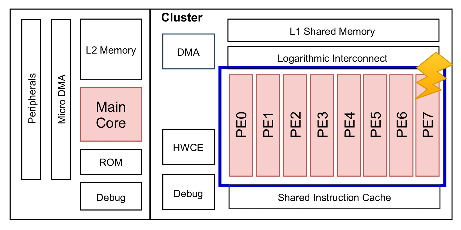
1, and so on. It is, thus, fairly straightforward to compute the number of critical neurons assigned to each PE. In our case study, the LeNet (MNIST) was scheduled on an AI-oriented multiprocessor SoC with 8 identical PEs (Figure 9). Hence, the workload of each layer was split into 8 chunks of neurons and statically assigned to the 8 PEs of the cluster. To determine the criticality of each chunk in a static scheduling, we relied on the final network-oriented score map and assigned a value to each chunk of neurons by computing the variance metric, i.e., Equation (4) described in Section 3.2. Figures are provided in Table 2. It should be noted that the numbers are converted into integers for complying with the next ILP-based methodology. The second column provides the total amount of neurons for each layer: each chunk is composed of that number divided by the available PEs. This reasoning cannot be applied for the last fully connected layer since there is not a precise division during the inference: having the neurons all connected between them, every PE elaborates all neurons. From the third to the last columns, the variance numbers are provided for each chunk of the layer. In the main, data in Table 2 suggest that the PE elaborating the highest quantity of critical neurons is PE0: the sum of the variances is equal to 83, the highest. On the contrary, PE7 is the one with least critical load: the sum of the variances is the lowest among the PEs and is equal to 28.
To prove the efficacy of the proposed scheduling as well as the reliability improvements of the targeted NCS (i.e., LeNet CNN running on GAP-8), a FI campaign was executed at the architectural level (RTL). We injected permanent faults (stuck-at-0 or stuck-at-1) into the RTL design of the PULP platform running the LeNet CNN.
A specific FI framework was built relying on a commercial simulator: Modelsim from Mentor Graphics. The reader should note that simulation-based FIs at RTL are computationally intensive and extremely time consuming. A single LeNet inference cycle at RTL took, on average, 25 min (the faults were placed in the GAP-8 RTL design so we could not take advantage of higher level FI frameworks). For this reason, massive injection campaigns were out of our computational scope. However, to speed up the RTL simulations, we exploited the pipelined fault injector proposed in [42]. It uses the pipeline concept to parallelize the inference cycles and introduces a high-level controller in Python language for moving the fault location and advancing the inferences. In the end, we were able to obtain an inference result about every 10 min. Despite the non-negligible FI time, the real advantage of simulation-based FIs at RTL is that they allow for the possibility of evaluating the NCS reliability before the fabrication process. In this way, the designer can coshape the software application with the target architecture to pursue a wished reliability level by carrying out precise injections on definite locations of the RTL architecture.
The choice of the faulty location was an arduous task. Indeed, when working at RTL, the injection locations are limited to some data path units, microarchitectural units such as registers [62] or memories. We bounded our analysis to the stuck-at faults on the inputs and outputs of the Flip-Flops composing the registers. In more detail, permanent faults were injected, one at a time, into the 8 RISC-V cores belonging to the cluster domain of the GAP architecture (as illustrated in Figure 9). To remark, the inference process was completely executed by the cluster’s cores (PEs) in a SIMD configuration. The main core sitting in the fabric controller area was only in charge of turning on the cluster, so assessing its reliability is out of the scope of this paper.
Faults were classified depending on their effect and in line with the ranking proposed in [34]. However, to cover the NCS in both the application and architectural level, we introduced a component-level metric, which is typically more connected to the hardware but, as suggested in [63], can be interestingly applied to classification problems: the mean squared error (MSE) of the output vector. Therefore, a fault was detected when one of the following situations occurred:
  • SDC-1: A silent data corruption (SDC) failure is a deviation of the network output from the golden network result, leading to a misprediction. Hence, the fault causes the image to be wrongly classified.
  • Masked with MSE > 0: The network correctly predicts the result, but the MSE of the faulty output vector is different from zero. It means that the top score is correct but the fault causes a variation in the outputs compared to the fault-free execution.
  • Hang: The fault causes the system to hang and the HDL simulation never finishes.
In the remaining cases, the fault was said to be masked with MSE = 0.
In particular, we propose an ILP and variance-based methodology to schedule portions of neural network layers on the available computing resources, to avoid critical portions of a network all being assigned to a single PE. The approach is described in Section 3.3 and takes as input the results shown in Table 2. It should be remarked that the variance figure for each chunk is fixed, regardless of the PE it is assigned to. Therefore, to obtain an optimal scheduling solution able to unify the “critical” load of the PEs, an ILP model was created by following (5)–(11), detailed in Section 3.3. Going into more detail, the constants were tuned to our target NCS, thus, P = 8 and L = 6. The reader should note that, as anticipated, the chunk assignment for fully connected layers does not make sense for topological reasons. Hence, in Table 2 the row L6 was excluded from the ILP formulation. Once all the formulas were created in a form suitable for the solver, they were passed to the ILP engine. The tool used was Opensolver [64], an open-source optimizer, and the specific optimization engine was CBC (COIN-OR Branch-and-Cut) solver. Apart from Table 2, the solver also takes the compilation constraints and the objective function as input. The outcome of the optimizer was the optimal scheduling shown in Table 3. As illustrated, the optimizer sorts the chunks so that the cumulative variance assigned to each PE during the whole inference cycle is uniformly distributed. Better solutions are not consistent with the integer constraints, which are crucial to comply with (7) and (9). Hence, the kernel of the PULP-NN library was changed to match the optimal scheduling order provided by the ILP solver. As discussed before, the chunks assignments to different PEs do not affect at all the final classification results.
The same set of permanent faults was injected in two scenarios: first, when the LeNet CNN application was compiled by following a static scheduling; then, when it was compiled with the proposed optimal scheduling.
A total of 164,000 RTL injections were performed. The same set of 2050 stuck-at-faults were injected in the cluster domain of the GAP-8 RTL design (as shown in Figure 9). Specifically, the injection targeted the register file of the cluster’s PEs. The injection procedure was the following. A set of 40 images was randomly selected from the MNIST test set. Then, a stuck-at-fault was injected into one of the PEs and the inference of the selected 40 images was performed by compiling the kernel functions of the CNN application with a static scheduling (a total of 82,000 inferences). Then, by keeping the same stuck-at-fault, the inferences of the same set of images was executed by compiling the kernel functions of the CNN application with the proposed scheduling (a total of 82,000 inferences).
As mentioned before, the pipelined framework was used for running the injections. By running 10 parallel processes, the 164,000 injections took about 41 days. The reader should note that for faults producing a simulation hang (i.e., 71,840 and 65,040 images in Table 4), the pipelined FI framework used a timer for avoiding the inferences of the full set of images.
The data illustrated in Table 4 show the capability of the proposed ILP and variance-based scheduling in improving the reliability of the NCS. For each row, the number of images that produce the corresponding effect in the static or proposed scheduling is reported along with the related percentage. It is necessary to underline that the new ILP scheduling leads to a 0.6% increase in memory occupation and an increase in simulation times of 3.2% at run-time for a single inference cycle. Nevertheless, the proposed ILP-based scheduling is able to reduce by 24.74% the neural network wrong predictions (SDC-1%). Moreover, as expected, the amount of correct predictions with MSE greater than zero (Masked, MSE > 0) increased by 97.80%. In other words, the new scheduling is able to reduce the risk of wrong predictions, producing, again, evidence of faults in the output vector (MSE > 0) but keeping the prediction correct. A third good point concerns the last row of the table (Masked, MSE = 0): the proposed scheduling is able to improve the masking ability of the neural network by 59.53%.

6. Conclusions

This paper provides a methodology to improve the reliability of a neural computing system running in a multi-core device. Through the paper, it was shown that it is possible to identify the most critical neurons of a neural network and, based upon this, determine an optimal scheduling for an AI-oriented MPSoC. Following the proposed methodology, it was experimentally demonstrated that not all ANN neurons play the same role in the final task. It is fair to say that neural networks are equipped with more neurons than needed, but which neurons to remove is the focus of the class-oriented analysis. On the heels of this study, we presented a technique to identify the ANN’s most critical neurons and sorted them according to their criticality. The experimental results show that our final sorting is more effective than those based only on a network-oriented analysis since we also consider the criticality of neurons with respect to the output classes. Relying on this analysis, the paper introduced an integer linear programming based mechanism, which takes into account the variance metric of portions of neurons. The aim was to uniformly distribute critical neurons to the available processing elements. The results of a further injection campaign at RTL provide evidence that the proposed scheduling can mask the effects of more faults and predict fewer wrong predictions. A reduction of 24.74% of wrong predictions and an improvement of 97.80% and 59.53% of masked faults was obtained. It is worth saying that, without resorting to any redundancy-based technique (either software or hardware), the reliability of a NCS and its tolerance to faults can be improved.
Future work will extend this analysis to deeper ANNs and different data sets. The reader should note that the adoption of the MNIST, SVHN, and CIFAR-10 data sets was consistent with the considered low-power and resource-constrained ASIC world. In the future, we will exploit deeper ANNs and more complex data sets, moving the target to GPUs and high-performance architectures or ad hoc hardware neural network chips. Clearly, with more complex neural networks, we need to study the feasibility of the uniform distribution and, if this cannot be satisfied, we will evaluate and propose different strategies that are well suited to deal with the complexity of the application. To conclude, in the future, we will address also other fault models, such as transient errors.

Author Contributions

Conceptualization, A.R. and E.S.; methodology, A.R. and E.S.; software, A.R.; validation, A.R. and E.S.; formal analysis, A.R.; investigation, A.R.; resources, E.S.; data curation, A.R.; writing—original draft preparation, A.R.; writing—review and editing, A.R. and E.S.; visualization, A.R. and E.S.; supervision, E.S.; project administration, A.R. and E.S.; funding acquisition, E.S. Both authors have read and agreed to the published version of the manuscript.

Funding

This research received no external funding.

Institutional Review Board Statement

Not applicable.

Informed Consent Statement

Not applicable.

Data Availability Statement

The data presented in this study are available on request from the corresponding author.

Conflicts of Interest

The authors declare no conflict of interest.

Abbreviations

The following abbreviations are used in this manuscript:
AIArtificial Intelligence
ANNArtificial Neural Network
DNNDeep Neural Network
CNNConvolutional Neural Network
ILPInteger Linear Programming
SoCSystem-on-a-chip
MPSoCMultiprocessor System-on-a-chip
ASICApplication Specific Integrated Circuit
SIMDSingle Instruction Multiple Data

References

  1. McCulloch, W.S.; Pitts, W. A logical calculus of the ideas immanent in nervous activity. Bull. Math. Biophys. 1943, 5, 115–133. [Google Scholar] [CrossRef]
  2. Sejnowski, T.; Delbruck, T. The Language of the Brain; Scientific American Volume 307; Howard Hughes Medical Institute United States: Stevenson Ranch, CA, USA, 2012; pp. 54–59. [Google Scholar] [CrossRef]
  3. He, K.; Zhang, X.; Ren, S.; Sun, J. Delving Deep into Rectifiers: Surpassing Human-Level Performance on ImageNet Classification. arXiv 2015, arXiv:1502.01852. [Google Scholar]
  4. Lawrence, S.; Giles, C.; Tsoi, A. What Size Neural Network Gives Optimal Generalization? Convergence Properties of Backpropagation. 2001. Available online: https://drum.lib.umd.edu/handle/1903/809 (accessed on 12 July 2021).
  5. El Mhamdi, E.M.; Guerraoui, R. When Neurons Fail. In Proceedings of the 2017 IEEE International Parallel and Distributed Processing Symposium (IPDPS), Orlando, FL, USA, 29 May–2 June 2017; pp. 1028–1037. [Google Scholar]
  6. Kung, H.T.; Leiserson, C.E. Systolic Arrays for (VLSI); Technical Report; Carnegie-Mellon University Pittsburgh Pa Department of Computer Science: Pittsburgh, PA, USA, 1978. [Google Scholar]
  7. Misra, J.; Saha, I. Artificial neural networks in hardware: A survey of two decades of progress. Neurocomputing 2010, 74, 239–255. [Google Scholar] [CrossRef]
  8. Palossi, D.; Conti, F.; Benini, L. An Open Source and Open Hardware Deep Learning-Powered Visual Navigation Engine for Autonomous Nano-UAVs. In Proceedings of the 2019 15th International Conference on Distributed Computing in Sensor Systems (DCOSS), Santorini Island, Greece, 29–31 May 2019; pp. 604–611. [Google Scholar] [CrossRef] [Green Version]
  9. Barkallah, E.; Freulard, J.; Otis, M.J.D.; Ngomo, S.; Ayena, J.C.; Desrosiers, C. Wearable Devices for Classification of Inadequate Posture at Work Using Neural Networks. Sensors 2017, 17, 2003. [Google Scholar] [CrossRef] [PubMed] [Green Version]
  10. Peluso, V.; Cipolletta, A.; Calimera, A.; Poggi, M.; Tosi, F.; Aleotti, F.; Mattoccia, S. Monocular Depth Perception on Microcontrollers for Edge Applications. IEEE Trans. Circuits Syst. Video Technol. 2021. [Google Scholar] [CrossRef]
  11. Ottavi, G.; Garofalo, A.; Tagliavini, G.; Conti, F.; Benini, L.; Rossi, D. A Mixed-Precision RISC-V Processor for Extreme-Edge DNN Inference. In Proceedings of the 2020 IEEE Computer Society Annual Symposium on VLSI (ISVLSI), Limassol, Cyprus, 6–8 July 2020; pp. 512–517. [Google Scholar] [CrossRef]
  12. Wolf, W.; Jerraya, A.A.; Martin, G. Multiprocessor System-on-Chip (MPSoC) Technology. IEEE Trans. Comput. Aided Des. Integr. Circuits Syst. 2008, 27, 1701–1713. [Google Scholar] [CrossRef]
  13. Ma, Y.; Zhou, J.; Chantem, T.; Dick, R.P.; Wang, S.; Hu, X.S. Online Resource Management for Improving Reliability of Real-Time Systems on “Big–Little” Type MPSoCs. IEEE Trans. Comput. Aided Des. Integr. Circuits Syst. 2020, 39, 88–100. [Google Scholar] [CrossRef]
  14. Desoli, G.; Chawla, N.; Boesch, T.; Singh, S.P.; Guidetti, E.; De Ambroggi, F.; Majo, T.; Zambotti, P.; Ayodhyawasi, M.; Singh, H.; et al. 14.1 A 2.9TOPS/W Deep Convolutional Neural Network SoC in FD-SOI 28 nm for Intelligent Embedded Systems. In Proceedings of the 2017 IEEE International Solid-State Circuits Conference (ISSCC), San Francisco, CA, USA, 5–9 February 2017; pp. 238–239. [Google Scholar] [CrossRef]
  15. Sim, J.; Park, J.; Kim, M.; Bae, D.; Choi, Y.; Kim, L. 14.6 A 1.42TOPS/W Deep Convolutional Neural Network Recognition Processor for Intelligent IoE Systems. In Proceedings of the 2016 IEEE International Solid-State Circuits Conference (ISSCC), San Francisco, CA, USA, 31 January–4 February 2016; pp. 264–265. [Google Scholar] [CrossRef]
  16. Flamand, E.; Rossi, D.; Conti, F.; Loi, I.; Pullini, A.; Rotenberg, F.; Benini, L. GAP-8: A RISC-V SoC for AI at the Edge of the IoT. In Proceedings of the 2018 IEEE 29th International Conference on Application-Specific Systems, Architectures and Processors (ASAP), Milan, Italy, 10–12 July 2018; pp. 1–4. [Google Scholar] [CrossRef]
  17. Venkataramani, S.; Ranjan, A.; Roy, K.; Raghunathan, A. AxNN: Energy-Efficient Neuromorphic Systems Using Approximate Computing. In Proceedings of the 2014 IEEE/ACM International Symposium on Low Power Electronics and Design (ISLPED), La Jolla, CA, USA, 11–13 August 2014; pp. 27–32. [Google Scholar] [CrossRef]
  18. Zhang, J.J.; Gu, T.; Basu, K.; Garg, S. Analyzing and Mitigating the Impact of Permanent Faults on a Systolic Array Based Neural Network Accelerator. In Proceedings of the 2018 IEEE 36th VLSI Test Symposium (VTS), San Francisco, CA, USA, 22–25 April 2018; pp. 1–6. [Google Scholar] [CrossRef] [Green Version]
  19. Bosio, A. Emerging Computing Devices: Challenges and Opportunities for Test and Reliability. In Proceedings of the 26th IEEE European Test Symposium (ETS), Bruges, Belgium, 24–28 May 2021; pp. 1–10. [Google Scholar] [CrossRef]
  20. Ramacher, U.; Beichter, J.; Bruls, N.; Sicheneder, E. Architecture and VLSI Design of a VLSI Neural Signal Processor. In Proceedings of the 1993 IEEE International Symposium on Circuits and Systems, Chicago, IL, USA, 3–6 May 1993; Volume 3, pp. 1975–1978. [Google Scholar] [CrossRef]
  21. Cappellone, D.; Di Mascio, S.; Furano, G.; Menicucci, A.; Ottavi, M. On-Board Satellite Telemetry Forecasting with RNN on RISC-V Based Multicore Processor. In Proceedings of the 2020 IEEE International Symposium on Defect and Fault Tolerance in VLSI and Nanotechnology Systems (DFT), Frascati, Italy, 19–21 October 2020; pp. 1–6. [Google Scholar] [CrossRef]
  22. Cerutti, G.; Andri, R.; Cavigelli, L.; Farella, E.; Magno, M.; Benini, L. Sound Event Detection with Binary Neural Networks on Tightly Power-Constrained IoT Devices. In Proceedings of the ACM/IEEE International Symposium on Low Power Electronics and Design; Association for Computing Machinery: New York, NY, USA, 2020; pp. 19–24. [Google Scholar] [CrossRef]
  23. Means, R.W.; Lisenbee, L. Extensible Linear Floating Point SIMD Neurocomputer Array Processor. In Proceedings of the IJCNN-91-Seattle International Joint Conference on Neural Networks, Seattle, WA, USA, 8–12 July 1991; Volume 1, pp. 587–592. [Google Scholar] [CrossRef]
  24. Dai, X.; Yin, H.; Jha, N.K. NeST: A Neural Network Synthesis Tool Based on a Grow-and-Prune Paradigm. IEEE Trans. Comput. 2019, 68, 1487–1497. [Google Scholar] [CrossRef] [Green Version]
  25. Sung, W.; Shin, S.; Hwang, K. Resiliency of Deep Neural Networks under Quantization. arXiv 2015, arXiv:1511.06488. [Google Scholar]
  26. Reagen, B.; Gupta, U.; Pentecost, L.; Whatmough, P.; Lee, S.K.; Mulholland, N.; Brooks, D.; Wei, G.Y. Ares: A Framework for Quantifying the Resilience of Deep Neural Networks. In Proceedings of the 55th Annual Design Automation Conference, San Francisco, CA, USA, 24–29 June 2018; Association for Computing Machinery: San Francisco, CA, USA, 2018; pp. 1–6. [Google Scholar] [CrossRef]
  27. Ruospo, A.; Bosio, A.; Ianne, A.; Sanchez, E. Evaluating Convolutional Neural Networks Reliability depending on their Data Representation. In Proceedings of the 2020 23rd Euromicro Conference on Digital System Design (DSD), Kranj, Slovenia, 26–28 August 2020; pp. 672–679. [Google Scholar] [CrossRef]
  28. Bushnell, M.; Agrawal, V. Essentials of Electronic Testing for Digital, Memory and Mixed-Signal VLSI Circuits; Springer Publishing Company, Incorporated: Berlin/Heidelberg, Germany, 2013. [Google Scholar]
  29. Torres-Huitzil, C.; Girau, B. Fault and Error Tolerance in Neural Networks: A Review. IEEE Access 2017, 5, 17322–17341. [Google Scholar] [CrossRef]
  30. Temam, O. A Defect-Tolerant Accelerator for Emerging High-Performance Applications. In Proceedings of the 2012 39th Annual International Symposium on Computer Architecture (ISCA), Portland, OR, USA, 9–13 June 2012; pp. 356–367. [Google Scholar] [CrossRef]
  31. Lotfi, A.; Hukerikar, S.; Balasubramanian, K.; Racunas, P.; Saxena, N.; Bramley, R.; Huang, Y. Resiliency of Automotive Object Detection Networks on GPU Architectures. In Proceedings of the 2019 IEEE International Test Conference (ITC), Washington, DC, USA, 9–15 November 2019; pp. 1–9. [Google Scholar] [CrossRef]
  32. Zhao, B.; Aydin, H.; Zhu, D. Generalized Reliability-Oriented Energy Management for Real-Time Embedded Applications. In Proceedings of the 2011 48th ACM/EDAC/IEEE Design Automation Conference (DAC), San Diego, CA, USA, 5–10 June 2011; pp. 381–386. [Google Scholar]
  33. Du, B.; Condia, J.E.R.; Reorda, M.S. An Extended Model to Support Detailed GPGPU Reliability Analysis. In Proceedings of the 2019 14th International Conference on Design Technology of Integrated Systems in Nanoscale Era (DTIS), Mykonos, Greece, 16–18 April 2019; pp. 1–6. [Google Scholar] [CrossRef]
  34. Li, G.; Hari, S.K.S.; Sullivan, M.; Tsai, T.; Pattabiraman, K.; Emer, J.; Keckler, S.W. Understanding Error Propagation in Deep Learning Neural Network (DNN) Accelerators and Applications. In Proceedings of the International Conference for High Performance Computing, Networking, Storage and Analysis; Association for Computing Machinery: New York, NY, USA, 2017. [Google Scholar] [CrossRef]
  35. Allen, C.; Stevens, C.F. An evaluation of causes for unreliability of synaptic transmission. Proc. Natl. Acad. Sci. USA 1994, 91, 10380–10383. Available online: https://www.pnas.org/content/91/22/10380.full.pdf (accessed on 12 July 2021). [CrossRef] [PubMed] [Green Version]
  36. He, Y.; Balaprakash, P.; Li, Y. FIdelity: Efficient Resilience Analysis Framework for Deep Learning Accelerators. In Proceedings of the 2020 53rd Annual IEEE/ACM International Symposium on Microarchitecture (MICRO), Athens, Greece, 17–21 October 2020; pp. 270–281. [Google Scholar] [CrossRef]
  37. dos Santos, F.; Draghetti, L.; Weigel, L.; Carro, L.; Navaux, P.; Rech, P. Evaluation and Mitigation of Soft-Errors in Neural Network-Based Object Detection in Three GPU Architectures. In Proceedings of the 2017 47th Annual IEEE/IFIP International Conference on Dependable Systems and Networks Workshops (DSN-W), Denver, CO, USA, 26–29 June 2017; pp. 169–176. [Google Scholar]
  38. Luza, L.M.; Söderström, D.; Tsiligiannis, G.; Puchner, H.; Cazzaniga, C.; Sanchez, E.; Bosio, A.; Dilillo, L. Investigating the Impact of Radiation-Induced Soft Errors on the Reliability of Approximate Computing Systems. In Proceedings of the 2020 IEEE International Symposium on Defect and Fault Tolerance in VLSI and Nanotechnology Systems (DFT), Frascati, Italy, 19–21 October 2020; pp. 1–6. [Google Scholar] [CrossRef]
  39. Bosio, A.; Bernardi, P.; Ruospo, A.; Sanchez, E. A Reliability Analysis of a Deep Neural Network. In Proceedings of the 2019 IEEE Latin American Test Symposium (LATS), Santiago, Chile, 11–13 March 2019; pp. 1–6. [Google Scholar] [CrossRef]
  40. Neggaz, M.A.; Alouani, I.; Lorenzo, P.R.; Niar, S. A Reliability Study on CNNs for Critical Embedded Systems. In Proceedings of the 2018 IEEE 36th International Conference on Computer Design (ICCD), Orlando, FL, USA, 7–10 October 2018; pp. 476–479. [Google Scholar] [CrossRef]
  41. Mahmoud, A.; Aggarwal, N.; Nobbe, A.; Vicarte, J.R.S.; Adve, S.V.; Fletcher, C.W.; Frosio, I.; Hari, S.K.S. PyTorchFI: A Runtime Perturbation Tool for DNNs. In Proceedings of the 2020 50th Annual IEEE/IFIP International Conference on Dependable Systems and Networks Workshops (DSN-W), Valencia, Spain, 29 June–2 July 2020; pp. 25–31. [Google Scholar] [CrossRef]
  42. Ruospo, A.; Balaara, A.; Bosio, A.; Sanchez, E. A Pipelined Multi-Level Fault Injector for Deep Neural Networks. In Proceedings of the 2020 IEEE International Symposium on Defect and Fault Tolerance in VLSI and Nanotechnology Systems (DFT), Frascati, Italy, 19–21 October 2020; pp. 1–6. [Google Scholar] [CrossRef]
  43. Cun, Y.L.; Denker, J.S.; Solla, S.A. Optimal Brain Damage. In Advances in Neural Information Processing Systems 2; Morgan Kaufmann Publishers Inc.: San Francisco, CA, USA, 1990; pp. 598–605. [Google Scholar]
  44. Han, S.; Pool, J.; Tran, J.; Dally, W.J. Learning Both Weights and Connections for Efficient Neural Networks. In Proceedings of the 28th International Conference on Neural Information Processing Systems; MIT Press: Cambridge, MA, USA, 2015; Volume 1, pp. 1135–1143. [Google Scholar]
  45. Wang, J.; Liu, L.; Pan, X. Pruning Algorithm of Convolutional Neural Network Based on Optimal Threshold. In Proceedings of the 2020 5th International Conference on Mathematics and Artificial Intelligence, Chengdu, China, 10–13 April 2020; pp. 50–54. [Google Scholar] [CrossRef]
  46. Lee, K.; Kim, H.; Lee, H.; Shin, D. Flexible Group-Level Pruning of Deep Neural Networks for On-Device Machine Learning. In Proceedings of the 2020 Design, Automation Test in Europe Conference Exhibition (DATE), Grenoble, France, 9–13 March 2020; pp. 79–84. [Google Scholar] [CrossRef]
  47. Liu, S.; Wang, X.; Wang, J.; Fu, X.; Zhang, X.; Gao, L.; Zhang, W.; Li, T. Enabling Energy-Efficient and Reliable Neural Network via Neuron-Level Voltage Scaling. In Proceedings of the 2019 IEEE 25th International Conference on Parallel and Distributed Systems (ICPADS), Tianjin, China, 4–6 December 2019; pp. 410–413. [Google Scholar] [CrossRef]
  48. Schorn, C.; Guntoro, A.; Ascheid, G. Accurate Neuron Resilience Prediction for a Flexible Reliability Management in Neural Network Accelerators. In Proceedings of the 2018 Design, Automation Test in Europe Conference Exhibition (DATE), Dresden, Germany, 19–23 March 2018; pp. 979–984. [Google Scholar] [CrossRef]
  49. Montavon, G.; Lapuschkin, S.; Binder, A.; Samek, W.; Müller, K.R. Explaining nonlinear classification decisions with deep Taylor decomposition. Pattern Recognit. 2017, 65, 211–222. [Google Scholar] [CrossRef]
  50. Hanif, M.; Shafique, M. SalvageDNN: Salvaging deep neural network accelerators with permanent faults through saliency-driven fault-aware mapping. Philos. Trans. R. Soc. Math. Phys. Eng. Sci. 2020, 378, 20190164. [Google Scholar] [CrossRef] [Green Version]
  51. Squire, L.R. Memory systems of the brain: A brief history and current perspective. Neurobiol. Learn. Mem. 2004, 82, 171–177. [Google Scholar] [CrossRef] [PubMed]
  52. Bosman, T.; Frascaria, D.; Olver, N.; Sitters, R.; Stougie, L. Fixed-Order Scheduling on Parallel Machines. In Integer Programming and Combinatorial Optimization; Lecture Notes in Computer Science (Including Subseries Lecture Notes in Artificial Intelligence and Lecture Notes in Bioinformatics); Nagarajan, V., Lodi, A., Eds.; Springer: Berlin, Germany, 2019; pp. 88–100. [Google Scholar] [CrossRef] [Green Version]
  53. Shmoys, D.B.; Wein, J.; Williamson, D.P. Scheduling Parallel Machines On-Line. In Proceedings of the 1991 Proceedings 32nd Annual Symposium of Foundations of Computer Science, San Juan, PR, USA, 1–4 October 1991; pp. 131–140. [Google Scholar] [CrossRef]
  54. Lee, J.H.; Jang, H. Uniform Parallel Machine Scheduling with Dedicated Machines, Job Splitting and Setup Resources. Sustainability 2019, 11, 7137. [Google Scholar] [CrossRef] [Green Version]
  55. Lecun, Y.; Bottou, L.; Bengio, Y.; Haffner, P. Gradient-based learning applied to document recognition. Proc. IEEE 1998, 86, 2278–2324. [Google Scholar] [CrossRef] [Green Version]
  56. Netzer, Y.; Wang, T.; Coates, A.; Bissacco, A.; Wu, B.; Ng, A.Y. Reading Digits in Natural Images with Unsupervised Feature Learning. In Proceedings of the NIPS Workshop on Deep Learning and Unsupervised Feature Learning; Curran Associates: Red Hook, NY, USA, 2011. [Google Scholar]
  57. Krizhevsky, A. Learning Multiple Layers of Features from Tiny Images. Technical Report. 2009. Available online: https://www.cs.toronto.edu/~kriz/learning-features-2009-TR.pdf (accessed on 12 July 2021).
  58. Paszke, A.; Gross, S.; Massa, F.; Lerer, A.; Bradbury, J.; Chanan, G.; Killeen, T.; Lin, Z.; Gimelshein, N.; Antiga, L.; et al. PyTorch: An Imperative Style, High-Performance Deep Learning Library. In Advances in Neural Information Processing Systems 32; Wallach, H., Larochelle, H., Beygelzimer, A., d’Alché-Buc, F., Fox, E., Garnett, R., Eds.; Curran Associates, Inc.: Red Hook, NY, USA, 2019; pp. 8024–8035. [Google Scholar]
  59. Sermanet, P.; Chintala, S.; LeCun, Y. Convolutional Neural Networks Applied to House Numbers Digit Classification. In Proceedings of the 21st International Conference on Pattern Recognition (ICPR2012), Tsukuba, Japan, 11–15 November 2012; pp. 3288–3291. [Google Scholar]
  60. Springenberg, J.T.; Dosovitskiy, A.; Brox, T.; Riedmiller, M. Striving for Simplicity: The All Convolutional Net. arXiv 2015, arXiv:1412.6806. [Google Scholar]
  61. Garofalo, A.; Rusci, M.; Conti, F.; Rossi, D.; Benini, L. PULP-NN: A Computing Library for Quantized Neural Network inference at the edge on RISC-V Based Parallel Ultra Low Power Clusters. In Proceedings of the 2019 26th IEEE International Conference on Electronics, Circuits and Systems (ICECS), Genoa, Italy, 27–29 November 2019; pp. 33–36. [Google Scholar] [CrossRef]
  62. Condia, J.E.R.; Reorda, M.S. Testing permanent faults in pipeline registers of GPGPUs: A multi-kernel approach. In Proceedings of the 2019 IEEE 25th International Symposium on On-Line Testing and Robust System Design (IOLTS), Rhodes, Greece, 1–3 July 2019; pp. 97–102. [Google Scholar] [CrossRef]
  63. Chandra, P.; Singh, Y. Fault Tolerance of Feedforward Artificial Neural Networks-A Framework of Study. In Proceedings of the International Joint Conference on Neural Networks, Portland, OR, USA, 20–24 July 2003; Volume 1, pp. 489–494. [Google Scholar] [CrossRef]
  64. Org, W.; Mason, A.; Dunning, I. OpenSolver: Open Source Optimisation for Excel. In Proceedings of the Annual Conference of the Operations Research Society of New Zealand, Auckland, New Zealand, 29–30 November 2010. [Google Scholar]
Figure 1. Proposed approach to improve the reliability of a neural computing system based on a MPSoC.
Applsci 11 06455 g001
Figure 2. The critical neuron identification process: a practical example with the MNIST data set.
Applsci 11 06455 g002
Figure 3. Static scheduling: Neurons assignment in a multiprocessor SoC.
Applsci 11 06455 g003
Figure 4. MNIST LeNet: software fault injection campaigns on random and critical neurons. A fixed percentage p of neurons is dropped.
Applsci 11 06455 g004
Figure 5. SVHN ConvNet: software fault injection campaigns on random and critical neurons. A fixed percentage p of neurons is dropped.
Applsci 11 06455 g005
Figure 6. CIFAR-10 All-CNN: Software fault injection campaigns on random and critical neurons. A fixed percentage p of neurons is dropped.
Applsci 11 06455 g006
Figure 7. Network-oriented analysis with a growing t percentage of critical neurons from the class-oriented analysis (CoA). A study on the influence of the CoA on the NoA with a growing t percentage.
Applsci 11 06455 g007
Figure 8. Showing the robustness of the proposed approach based on the contribution of the CoA and the NoA (blue lines).
Applsci 11 06455 g008
Figure 9. Overview of the GAP-8 architecture and RTL fault injection location.
Applsci 11 06455 g009
Table 1. ANN benchmarks.
CNN ModelData SetApplicationAccuracyTotal Neurons
Custom LeNet-5MNISTImage Classification99.3148,650
ConvNetSVHNObject Recognition92.01185,374
All-CNNCIFAR-10Object Recognition90.57361,046
Table 2. Figures of variance when the chunks of neurons are assigned following static scheduling.
Chunks Variance-Static Scheduling
LayerNeuronsPE0PE1PE2PE3PE4PE5PE6PE7
L032,7681210865564
L18192311112112110185
L240961815179138119
L31024197325623
L4204813344444
L551211221122
L61011111111
Total48,6508348463550354428
Table 3. Figures of variance when the chunks of neurons are assigned following the proposed ILP and variance-based optimal scheduling.
Chunks Variance-Proposed Optimal Scheduling
LayerNeuronsPE0PE1PE2PE3PE4PE5PE6PE7
L032,7688664551210
L18192215103118121111
L240969915813171118
L31024319725632
L4204844313444
L551212111222
L61011111111
Total48,6504746434846474448
Table 4. RTL fault injection results: Evaluation of the effects of the same permanent faults on a CNN compiled with two different scheduling methods.
Fault Injection ResultsStatic SchedulingProposed Scheduling[%] Variation
Images[%]Images[%]
SDC-113381.6310071.23−24.74
Hang71,84087.6165,04079.32−9.47
Masked, MSE > 049105.99971211.84+97.80
Masked, MSE = 039124.7762417.61+59.53
Total82,00010082,000100
Publisher’s Note: MDPI stays neutral with regard to jurisdictional claims in published maps and institutional affiliations.

