Abstract
In a demanding and globalized market, production management plays a fundamental role in the company’s reference. Proper management of the production area allows companies to obtain productivity gains, reducing operational costs and make contributions to face the competitiveness of their competitors. When defining its strategic objectives in a productive system, it is necessary to formulate plans to manage human resources and strategies based on requirements. In this context, planning, production, and control (PPC) is an excellent ally of the organizations. The adequate development of the activities of the PPC allows companies to minimize production orders not attended, minimize stocks of raw materials, and finished products, minimize idleness of human resources by efficient allocation of work and minimize production processing times. The present work proposes a study to organize and develop a model that guides the prediction of the setup gain in the fabric dyeing process, structured by the traveling salesman problem.
1. Introduction
Globalization crosses borders, and free trade intensifies between countries. As a result, many sectors of the economy benefited from trade barriers that limited import and export quotas find themselves threatened by foreigners. In this sense, the threat of new entrants implies competition for market share, reduced margins, better performance, quality, cost, productivity, and operational efficiency. According to [1], these factors are essential for companies to be consistently inserted as new competitive dimensions.
In conjunction with coordinated and integrated operational management, an organization’s livelihood depends on its financial and economic results. Thus, resource management aimed at reducing costs without compromise the benefit to customers. These resources must be managed efficiently, minimizing waste and costs, and maximizing profits [2].
In this context, a planning area plays a fundamental role in the company’s strategy, coordinating the flow of information so that available resources are directed to serving the end customer at the lowest cost. To seek efficient use of resources, companies are increasingly using tools and methods to support decision making [3].
It is no different in the textile and clothing sector, as it has been suffering from the loss of market share for imported products and its low operational efficiency. The sector presents a high complexity in the planning process due to the vast portfolio of products needed to meet the dynamism of the fashion market. Serving this market requires a lot of flexibility in the production process that can often compromise its operational efficiency, so the quality of the preparation of the production schedule impacts productivity, intermediate stocks, quality, and billing.
According to [4], Brazil holds the most extensive integrated textile chain in the West, ranging from the production of fibres, through cotton plantations, for example, to fashion shows, going through all industrial processes such as spinning mills, weaving, finishing, clothing, and retail. Among the different types of fabrics produced, the study turns its attention to the production of denim, a kind of fabric that is the basis to produce jeans.
Nowadays, most textile industries use automated equipment for scale and quality. In the context of the fourth industrial revolution, the textile industry seeks to expand from automation to planning and scheduling tasks [5]. Until the mid-1960s, many papers published assumed that setup time (cost) was not necessary. However, this assumption simplifies the analysis and compromises the solution quality of many scheduling applications requiring appropriate treatment of setup time (cost) [6].
Setup times are significant in the textile industry and should be considered as separated. Fabrics are produced on looms with specific adjustments, and when this fabric is changed, the loom must be adjusted accordingly, consuming time that is a scarce resource [7].
Given the context presented, the following research question arises:
- How to improve the scheduling of the fabric dyeing process by optimizing setup times?
This research is positioned in the operational research (OR) in mathematical programming involving integer programming models. It aims to present a solution model for the production scheduling problem applied in a confirmed case of fabric dyeing scheduling, structured in the traveling salesman problem, to optimize the setup. The purpose of this research goes beyond the comparison between scheduling methodology, and it aims to obtain a formulation that can be replicated in companies of the same segment.
The remainder of the paper is structured as follows. Section 2 presents a literature review with the main concepts, definitions, and approaches on the Brazilian textile sector, planning production control and operational research. Moreover, Section 3 focuses on research methodology, with its characterization and structuring choose the representative features for simulation and comparison between the optimized model and empiric model. Besides, Section 4 shows the evaluation model’s structuring, containing the relationship of the result with the parameters. Finally, Section 5 concludes with results and discussions of this application, followed by a conclusion.
2. Brazilian Textile Sector
Denim is a popular fabric that no other fabric has received such a wide acceptance [8]. Today, Brazil is a world reference in beachwear, jeanswear and homeware design, with the fitness and lingerie segments has also grown. The sector is one of the largest employers in the country, accounting for about 1.5 million direct jobs, equivalent to 21% of the total workers allocated to industrial production in 2019, reinforcing the sector’s importance for the economy in general. In that same year, the textile chain produced approximately BRL186 billion, equivalent to 7% of the total production value of the Brazilian transformation industry, excluding the mineral extraction industries and civil construction activities [9].
Domestic production is practically directed to meet domestic consumption, but a relevant portion of what is consumed internally is imported. Analyzing the imports of the entire textile chain from 2015 to 2019, there was an increase of 20.7% in volume but a drop of 10.7% in value. There was an increase of 56.4% in volume and 29.9% in value in the fibre and filament segment. On the other hand, textile manufacturers advanced 4.5% in volume and retreated 8.8% in value, while in manufactured goods, there was a drop of 3.7% in volume and 25.2% in value. The behaviour of imported apparel, which fell in both types, is due to competition with domestic production in the period, which was more advantageous for purchase after the increase in imported products [9].
2.1. Manufacture
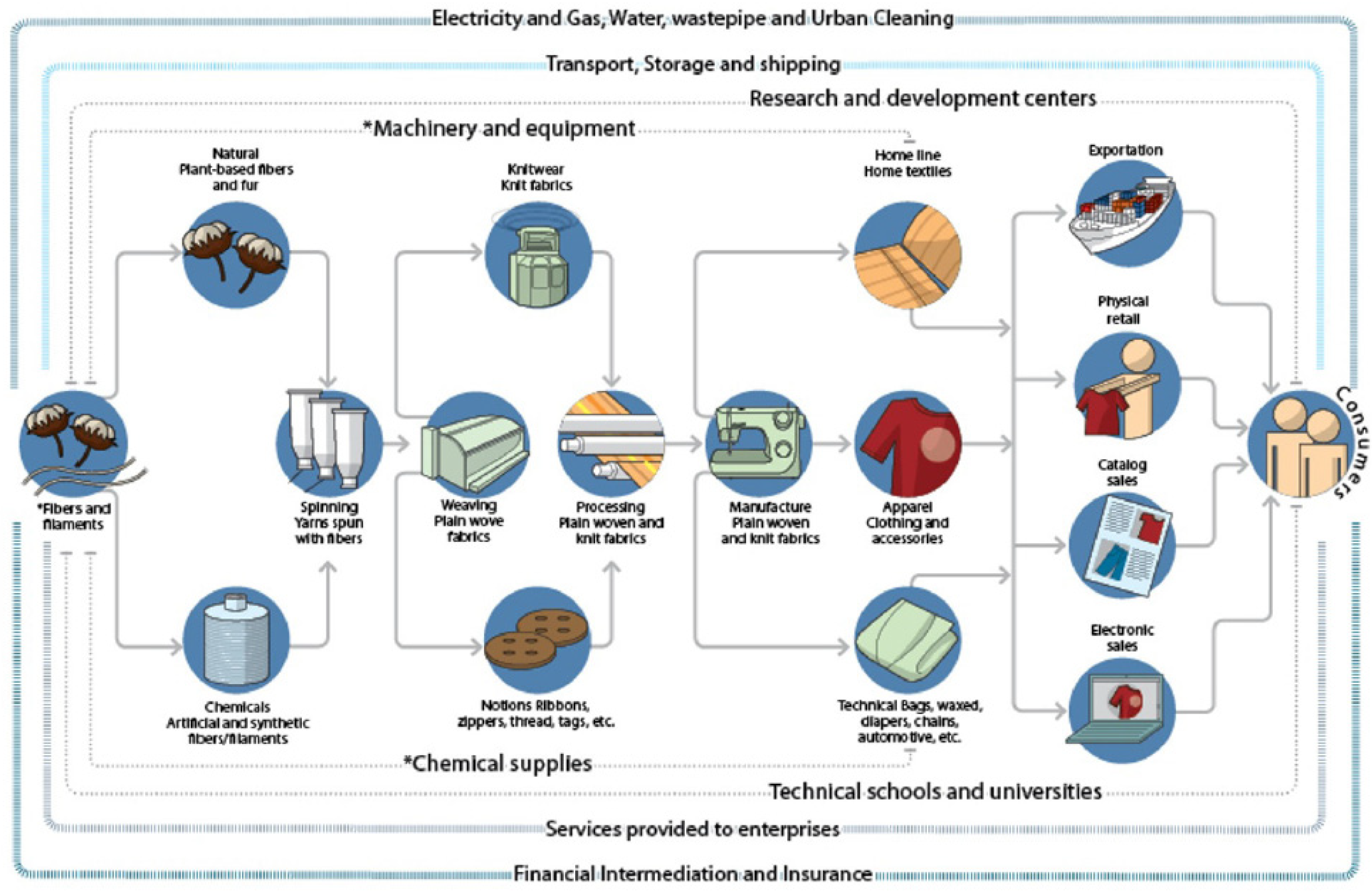
The textile chain starts transforming the raw material (natural, synthetic fibres and polymers) into yarns and filaments in the spinning mills. Then there can be two flows, first: warping, dyeing, flat weaving, finishing, and finally the clothing phase, and second: knitting, finishing, and finally the clothing and distribution phase. In Figure 1, we can see the macro flow of the chain. Thus, the result of each step constitutes the primary input of the next one. Each stage has its characteristics, with discontinuity between them, subdividing into several operations and elaborating intermediate products.

Figure 1.
Structure of the textile and apparel production and distribution chain.
The dyeing sector stands out as a critical process in operation and with many opportunities for gain. Beyond the technical aspect, there have been concerns about minimizing the negative environmental impact of the dyeing industry. For this production, scheduling has been applied [10] in many process industries for reducing pollutions emissions. Denim manufacturing faces an eco-efficiency challenge concerning sustainability. Alternatives have been studied to develop new dyeing processes that are cleaner, more efficient, faster, cheaper, and easier to apply [8].
The dyeing process of denim type fabrics (used to make jeans) is characterized by dyeing the cotton yarn before weaving [11]. In this process, the most used dye is indigo, whose method remains the same as natural indigo [12].
In the continuous indigo dyeing process, there are three technologies, which are:
- Rope dye
- Slasher dye
- Loop dye
2.2. Planning Production Control
The problem of timing and sizing production lots are frequently in several companies. These setup operations, like switching between production batches, machine adjustments, and cleansing procedures over a given planning horizon, are critical because the sequencing influences the consumption time and raises costs [8]. Sequencing establishes the order in which lots are executed within a period, accounting for the sequence-dependent setup times and costs. Integration of lot sizing and sequencing enables the creation of better production plans. Production plans can minimize the overall costs of stock holding and setups while satisfying the available capacity in each period from which the expenditure in setup times is deducted [13].
Planning production control (PPC) is responsible for coordinating a company’s productive resources to meet market demands, reconciling internal limitations (production and financial capacity) and assisting in the organization’s decision-making, such as stock policies, service level in service and cost reduction [14].
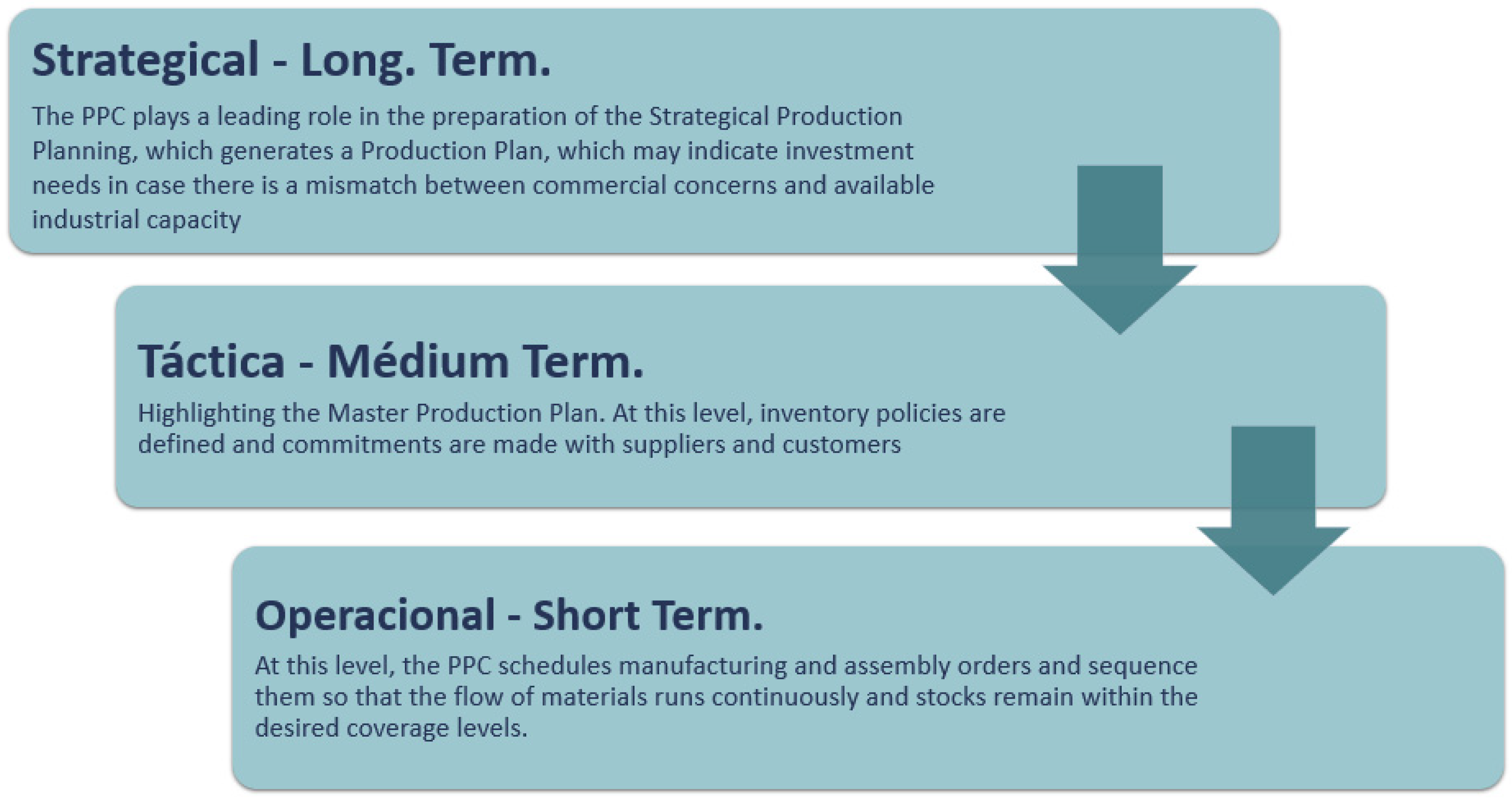
According to [15], the PPC performs activities at three different hierarchical levels. Each level varies according to the time horizon understudy, as shown in Figure 2.

Figure 2.
Hierarchical level of activities.
PPC is responsible for managing the flow of information through various production systems to meet best the plans established at the strategic, tactical, and operational levels.
2.3. Operational Research
The growth and complexity of organizations that emerged after the industrial revolution led to a division of labor and fragmentation of managerial responsibilities. Although this fragmentation of tasks has generated excellent results, in many cases, different sectors have their own goals and values, losing sight of the organization’s functioning. The organization of the operations of these large corporations made new methodologies popular. Among them, we highlight the scientific approach called operational research (OR), which aims to solve decision-making problems through typically mathematical models, whether deterministic or probabilistic [16].
According to [17], OR is characterized using scientific and quantitative methods by interdisciplinary teams to seek the best use of scarce resources and optimize and coordinate the operation of a company.
2.3.1. Integer Programming
For a problem to be classified as an integer programming (IP) problem, all decision variables in the model must be discrete. They can assume values within a finite set or a countable amount of importance derived from a count. When part of the decision variables is discrete, and the others are continuous, the model is called mixed integer programming [18].
In cases where all decision variables are binary, they can only assume values of 1 or 0. There is a Binary Programming model. Further, when part of the decision variables is binary, and the others are continuous, there is a mixed binary programming model. Furthermore, when the model has decision variables, discrete and binary, there is a binary integer programming problem [18].
Task assignment problems are examples of binary programming, including backpack problem, traveling salesman problem, vehicle routing problem, among others. As an example of IP, there is the problem of staff scheduling, and as an example of the mixed binary problem, there is the problem of the location of facilities [18].
2.3.2. Traveling Salesman Problem
The travelling salesman problem (TSP) is one of the most widely studied problems in the combinatorial optimization area [19]. TSP is interesting not only from a theoretical point of view but because of the various practical applications that can be modelled by the problem or its variations, with the need to find an efficient algorithm to solve it, among the most valuable applications known from the TSP, stand out the sequencing of the machine operations in manufacturing, optimization of hole drilling in printed circuit boards and most vehicle routing problems [20]. According to [13], it can be an essential source of ideas for developing more efficient models and scheduling problems. Similarities between TSP and the sequencing problem allow for direct manufacturing, where the city would be a job. The distance between one city and another would be the time (cost) of moving from one job to another [21].
We can describe the problem as follows: a travelling salesman has the task of visiting a set of cities, with each pair of cities i and j having an associated cost, representing the distance to travel from city i to city j. The salesman must depart from an initial town, visit all other cities once and return to the city of departure, completing a Hamiltonian Cycle at the lowest possible cost or the shortest trajectory.
There are several formulations for the TSP, and these formulations can be considered canonical because it is a classic optimization problem widely spread in the specialized literature and because they develop peculiar ways of characterizing the problem. To simulate the dye sequencing to obtain the shortest setup time, the TSP model was used, with the approach proposed by Miller–Tucker–Zemlim (MTZ) formulation, with the contribution of [22,23], for the elimination of sub-routes, because according to the latter, the MTZ formulation is vulnerable to the relaxation of constraints. This model was chosen because it works with a limited number of restrictions.
subject to:
The formulation of elimination of subtours proposed by MTZ, can be expressed by:
The formulation of elimination of sub tours proposed by MTZ can be strengthened using the elevation technique [22].
Equation (1) represents the objective function to minimize the total cost of the salesman route, where is the cost or distance of the arc i, j and is the binary variable (0 or 1) that decides whether route i, j will be included in the problem’s solution or not. Equations (2) and (3) refers to constraints that ensure that each node or vertex has only one input and only one output to the optimized graph.
Moreover, Equations (4) and (5) prevent the travelling salesman, saw more than n cities on a trip (a trip we understand, as visiting all the cities without passing through the city origin). In addition, and, are non-negative variable, which represents the number of cities visited before returning to the city of origin. However, it still does not guarantee the existence of sub tours, that is, two or more graphs disconnected from each other. Thus, adding a set of constraints like Equation (6) on the possible sub tours of the problem does not contain enough edges to make them closed loops.
3. Structuring the Problem Assessment Model
In this section, will be presented the methodological aspects necessary for the research to reach the proposed objectives are addressed. The section is divided into four parts, starting with the research characteristics and then by the three phases of study construction: informative, development and application.
On the other hand, this research is applied because it aims to develop a study to reduce setup time in a dyeing process in the textile industry, and with a qualitative–quantitative approach, as it will use statistical resources and techniques and will have interactions with experts from process and researchers to legitimize the information gathered and generate practical knowledge.
This research is characterized as a case study in the denim textile industry, and analyzes will be carried out on documents, data collection, identifying the current sequencing process of the dyeing schedule, and the impacts of the application of setup optimization cost and time availability.
Then, an optimizer processed these data that proposed an optimal fabric dyeing scheduling, whose objective function is to reduce the total setup time. Subsequently, the two situations (empirical and optimized) were compared to measure the financial impact and the factors that correlate to the outcome of the problem.
Regarding data collection, they were collected from the company’s database, parameterized from 1 February 2018 to 30 November 2018. This period was chosen because production took place uniformly throughout the year, unlike 2019 and 2020, when there was a substantial recession in the textile sector followed by the coronavirus pandemic, which would undoubtedly compromise data quality. In addition, January and December are months of return from vacations and deceleration of production for the beginning of holidays.
3.1. Informative
This research is structured in three data collection instruments: bibliographic research, electronic research, and interviews. For [24], bibliographical research is intended to put the researcher in contact with everything that has been produced on the subject.
This study began with searching for the existing theoretical framework on the subject in question, with a systematic literature review being carried out, selecting books, journal articles, doctoral theses, and master’s dissertations, which had some degree of impact on the research.
3.2. Development
The structuring phase began with electronic research through data collection in the company’s information system. The report used to obtain the data was parameterized for the period from 1 February 2018 to 30 November 2018. This report could extract the accurate dyeing scheduling, type of SKU (stock keeping unit) processed, the machine used, and the processing date. Then, interviews were conducted with experts in dyeing and PPC through brainstorming, as shown below.
- (a)
- Step 1—Interview with dyeing experts
At this stage, interviews were conducted with experts in the dyeing area to review and structure the setup time matrix.
- (b)
- Step 2—Interview with PPC and dyeing experts
At this stage, a brainstorming session was carried out between the PPC and dyeing team members to define the factors that could most influence the dyeing setup time. After brainstorming, the PPC and dyeing teams evaluated three factors as the most relevant: machine group, SKU number and programming horizon. It is believed that there is a correlation between these factors and setup time.
3.3. Application
For the study of setup time scheduling, the traveling salesman problem methodology was chosen, as it was seen the opportunity to employ a classic problem, which consists of searching for a circuit that has the shortest distance, passing through n cities, starting from any city, visiting all the others once and returning to the city of origin. In the study in question, the SKUs will represent the cities, and the setup time between pairs of SKUs will represent the distance between cities.
Considering that the analysis aims to create a model that guides the prediction of setup time gain, comparing the optimized method with the empirical method, the tests were performed within a set of configurations, parameterized by factors that are subject to change, and which may influence the result of the optimization.
The factor is:
- Machine group: despite not being input to the problem, it deserves attention because the analyzed samples were processed in two groups of machines: slasher dye, being more complex and larger machines for more elaborate dyeing, and loop dye are smaller machines with a more straightforward conception and low-cost dyeing, so the two groups must be analyzed separately.
- Number of SKU: this factor is susceptible to seasonality and can vary significantly depending on fashion trends and market demand.
- Programming horizon: the further we can see the demand, the greater the optimization opportunities, so for each composition of machine group and SKU number, tests were performed for different horizons, ranging from one to four weeks.
4. Evaluation Model
According to [25], a model represents an object, system, or idea in some form other than the entity itself and aims to understand the characteristics of the real system better.
We can consider two ways to solve the sequencing problem using TSP, the first one, considering that each SKU will be produced only once per cycle, and determining the sequence that minimizes the total setup. Furthermore, the other way is to establish a finite number of production runs for a given number of SKUs. An SKU can be programmed more than once in the cycle and then determine the runs that optimize the total setup [26].
Bringing this model to the case of fabric dyeing scheduling, the matrix VxV with elements are considered, where V represents the total of SKU number, and the setup time necessary to adjust the machine to the SKU j, from that the SKU i was produced immediately before. Given this condition, it is possible to form a cycle with the V SKUs taking their respective as for arc length [27].
4.1. Structuring Setup Time Matrix
The company studied is composed by two groups machines, slasher dye group and loop group.
The preparation of the setup time matrix was structured from the survey of the SKUs processed throughout 2018. From the knowledge of the SKUs processed in each dyeing machine, it was possible to structure a setup time matrix filled in by the area’s technical coordinator, with setup times for each likely SKU pair.
The setup time matrix was building for each machine of the company, and Supplementary Material Table S1 shows an application of a VxV matrix with 38 SKU’s for a machine from the loop dye group.
It can be observed a particularity that distinguishes it from a distance matrix between cities, according to the classic TSP, which has its principal diagonal equal to zero, since the distance to go from city i to the city i is equal to zero. In the case of the dyeing process, the dyeing batches are finite. At the end of each batch of a given SKU, it is necessary to restock the machine with a new load of yarn, prepare dye baths and calibrate the control points of the machine, even if the next batch refers to the same SKU processed previously, so the setup time between pairs of the same SKU will be greater than zero, but less than or equal to the setup time between different pairs of SKUs. Only six machines were eligible for the study from the company’s industrial park, as the others had the exact setup times. Thus, the study was based on three machines from the slasher dye group and three machines from the loop dye group.
4.2. Structuring for Test
To achieve the objectives of the research, which proposes the creation of a model that guides the prediction of reduced setup time, with the adoption of optimization tools, it is necessary to carry out a certain number of tests, in different process configurations, to generate a quantity of data that can provide a function capable of responding to most situations that may be encountered.
As mentioned before, it was evaluated those three factors are relevant to the operation, namely: machine group, SKU number and planning horizon. As the machine groups are already known (slasher dye and loop dye) and we know that the planning horizon will vary from one to four weeks, it remains to define the number of SKUs. For this, an analysis was carried out on the company’s data to identify the number of processed SKUs by the dyeing machine throughout 2018. According to Table 1, we can identify each machine, the number of dyeing batches and the SKU number processed throughout the month. A single SKU can be processed more than once throughout the month, so the number of batches is greater than the number of SKUs.

Table 1.
Number of processed SKU.
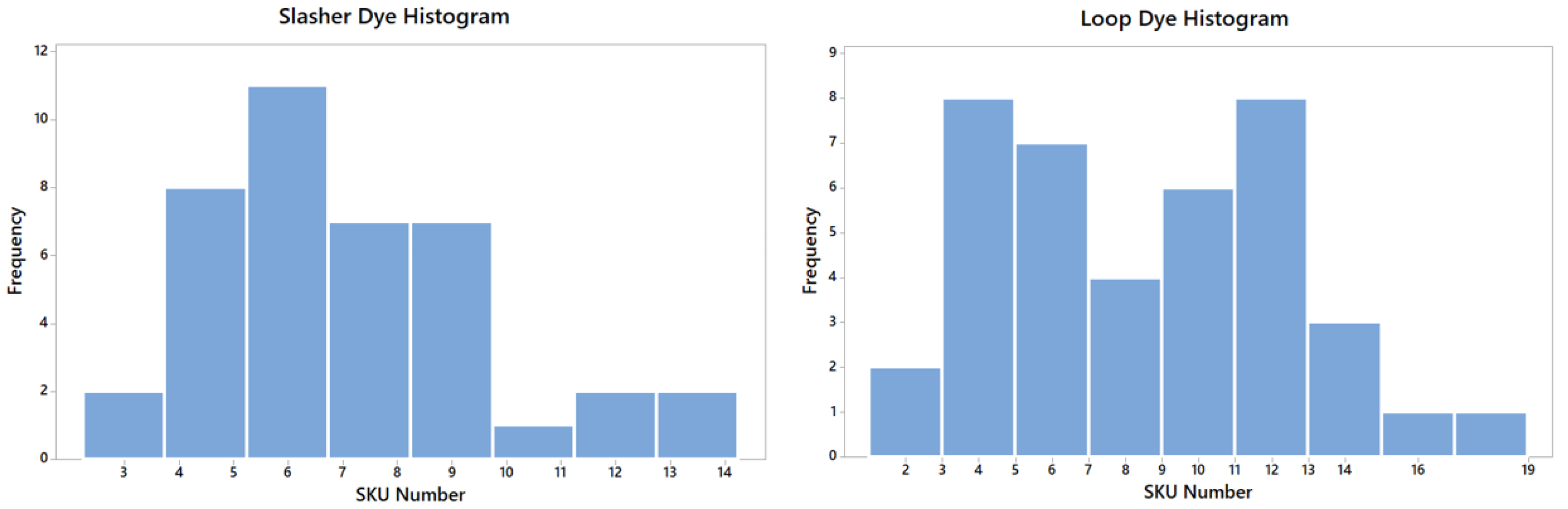
From these data, it was possible to build a histogram demonstrating the frequency of the number of processed SKU per month for the two groups of machines, as shown in Scheme 1. The importance of this parameter is due to its variability throughout the year, mainly due to market seasonality and fashion trends. Thus, a range of SKU quantities to be tested was defined, which could guarantee a good range of results.
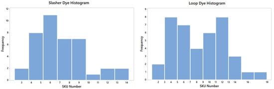
Scheme 1.
Frequency of the number of processed SKUs per month.
The histograms were thought to select many SKUs for testing to obtain a range of results, which serve as parameters for constructing a linear regression equation. This can be used in other companies with the same similar process.
Therefore, for the slasher dye group, the SKU number defined was: 4, 6, 8, 9 and 12. As for the loop dye group, the SKU number was: 5, 7, 9, 11, 12, 13 and 16. This dataset should cover the possible occurrences. Table 2 shows how the configurations of the number of SKUs per dye machine were structured.
Table 2.
SKU numbers were chosen to test.
With the definition of these configurations, it was possible to advance the measurement of setup times according to the empirical sequencing through the company’s reports. From the report, it was possible to extract, for each machine, the processing sequence throughout each month, fractionate the horizons. With the setup time matrices, it was possible to measure the setup time to go from SKU i to SKU j.
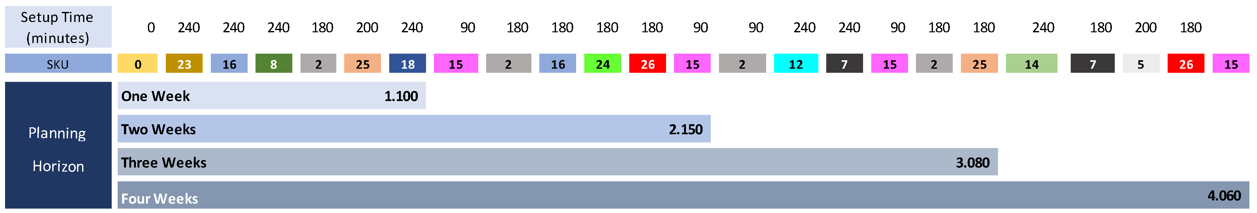
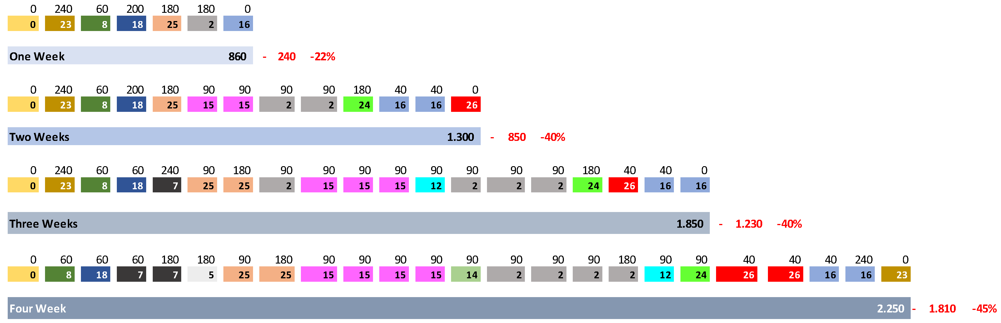
A total of 52 tests were carried out, 24 tests for the slasher dye machine group and 28 tests for the loop dye machine group. Figure 3 shows an example of setup time measurement performed on machine 7, with 13 SKU, broken down into four horizons.

Figure 3.
Measurement of setup time–machine seven from loop dye group, 13 SKU.
It is adapting the TSP model to the case study, starting from the need to produce a given amount of n dyeing batches for each SKU, which must be sequenced to obtain the shortest setup time, represented by in the Equation (1). There will be situations that, for the same SKU, the demand will be greater than one dyeing batch. Thus, for each batch to be processed, its code will be indexed to construct the setup time matrix. In this way, the same SKU can appear more than once in the matrix.
To ensure a better understanding, let’s take the situation illustrated in Figure 3, where the development of actions to optimize the sequencing of machine seven of the loop group will be presented.
For the machine in question, tests were performed for three SKU situations, as shown in Table 2. However, it is enough to describe only one situation for a good understanding, as the rationale is the same for all other cases. Therefore, the situation with 13 SKUs will be described, where the reference month was August 2018, as shown in Table 1.
The main matrix was built with all the SKUs processed on Machine 7. As shown in Supplementary Material Table S1, it was possible to build the setup time matrix for each programming horizon, according to Table 3, Table 4 and Table 5.
Table 3.
Setup time matrix for one and two weeks, Machine 7, 13 SKUs.
Table 4.
Setup time matrix for three weeks, Machine 7, 13 SKUs.
Table 5.
Setup time matrix for three weeks, Machine 7, 13 SKUs.
It can be noted that a SKU was incorporated into the setup time matrix that was called zero and that it has a setup time equal to zero to any other SKU. This device was used so that when completing a sequencing cycle, the return from the last processed SKU would go to SKU 0 because in the real situation, a new sequencing would hardly start from the SKU that was the origin of the previous sequencing.
For the simulations, LINGO software was used, version 17, licensed educational version, and the implementation was performed on a Dell branded equipment, i7 processor, 16 Gb, SSD.
After processing the data in the simulator, the results obtained can be viewed in Figure 4.
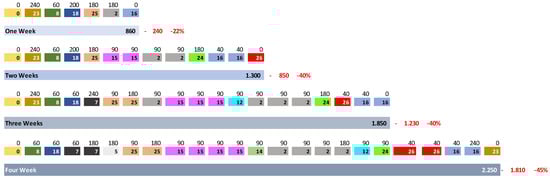
Figure 4.
Optimized result for Machine 7, from the loop dye group, 13 SKUs.
Figure 5 presented by the LINGO software [28], shows the fill-in of the matrix model composed of values in zeros and ones, varying only in the number of variables and constraints.

Figure 5.
Fill-in approach to the model matrix.
Considering that this is the application of the traveling salesman problem, there is a limitation of the problem considering that it is a large problem that may involve thousands of variables and restrictions. In this aspect, it is necessary to research the possibility of applying large scale decompositions, namely, Benders, Danzig–Wolfe or cross-decomposition decompositions, to the traveling salesman problem to obtain an exact solution. Other options are structured in hybrid methods [29].
For large models structured, considering the traveling salesman problem approach becomes necessary for other methodologies [30,31,32].
After measuring the setup times for all the suggested settings in four kind horizons, one week, two weeks, three weeks and four weeks, the SKU number referring to the whole horizon, we came to Table 6.
Table 6.
Results of slasher dye and loop dye group, accurate and optimized setup times.
The collected data made it possible to analyze the correlation between the setup time variation with the parameters, machine group, SKU number, and programming horizon. The information obtained was submitted to estimate the linear correlation coefficients (r) using the Minitab 17 software.
The linear correlation coefficient, sometimes called Pearson’s product moment correlation coefficient, is represented by the letter r and takes values from −1 to 1 and measures the degree of the linear relationship between the paired values x and y in a sample. When r = 1, it represents the perfect and positive correlation between two variables, and for r = −1, it means a perfect negative correlation between two variables. That is, while one increases, the other decreases [33].
The Pearson’s correlation coefficient is calculated according to the following formula:
where: n—represents the number of data pairs present; x, y—are the sample values you want to evaluate the correlation.
The analysis was performed separately for each machine group, and the correlation between % variation with the number of SKU and % variation with the programming horizon was evaluated. Absolute variation with SKU number and absolute variation with programming horizon.
Below in Table 7 are presented the results obtained for the two groups of machines.
Table 7.
Linear Correlation Coefficient.
It was chosen to study the correlation of both the relative variation and the absolute variation of setup times to assess possible divergences in the behaviour of the linear correlation coefficients. As it can be seen, there is a difference in the reading of information between the two situations.
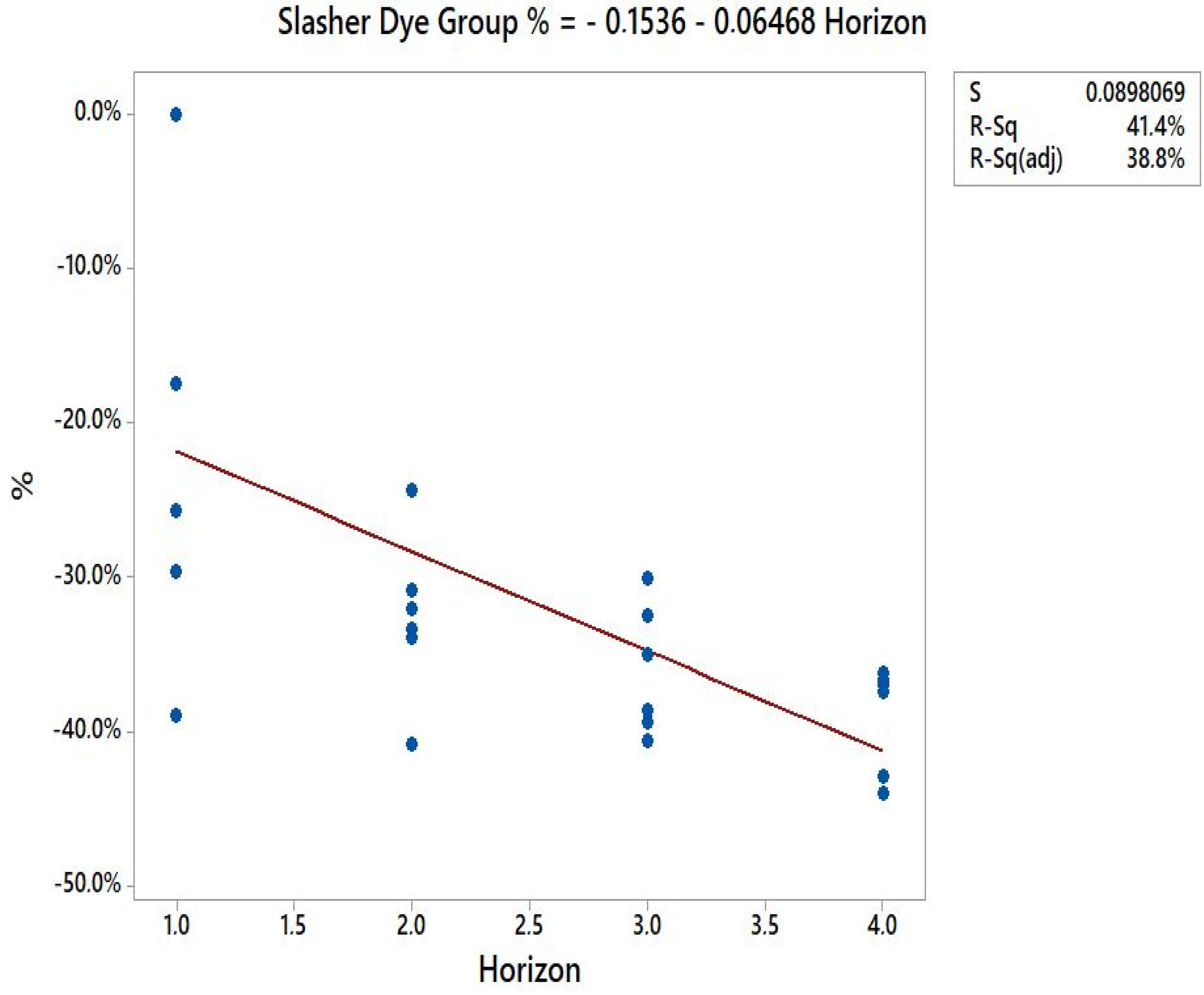
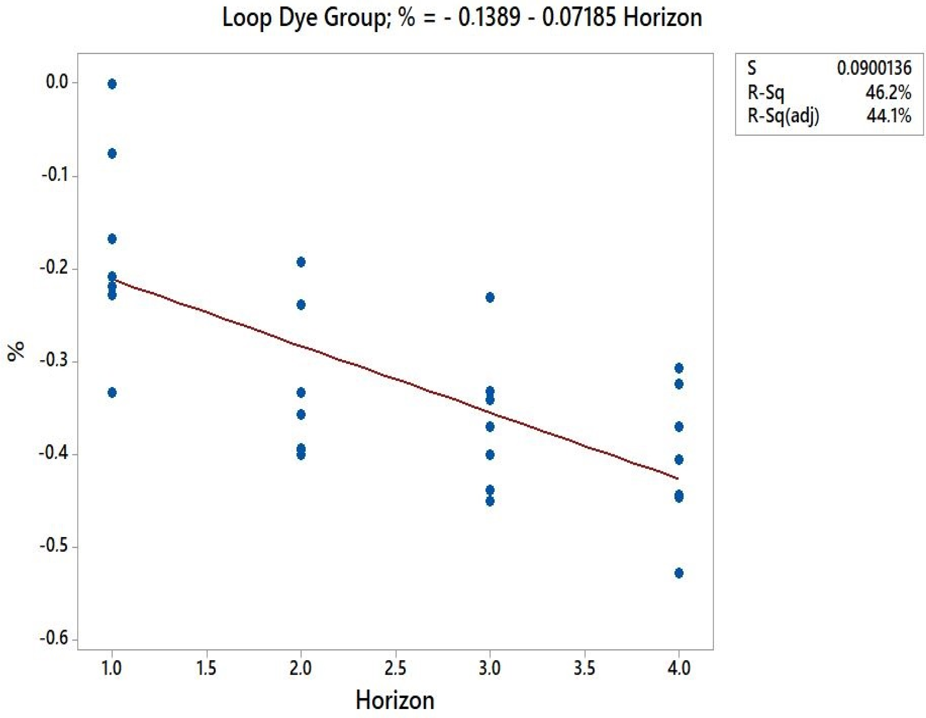
Contrary to what was expected, the correlation of the number of SKUs with variation in setup time presented practically null correlation coefficients for both machine groups. That is, there is no correlation between the number of SKUs with variation in setup time. However, the planning horizon showed a strong negative correlation with the interpretation in setup time, with the value of r for slasher dye and loop dye group for the relative variation being −0.644 and −0.679, respectively. For the absolute deviation, it was −0.928 and −0.859, respectively. That is, the absolute variation presented a more substantial relationship degree with the planning horizon. The negative correlation shows that, as the planning horizon increases, the optimization system is more efficient is in reducing setup time. In a way, this result was already expected, as not only in dyeing sequencing, as in other areas, the more you can anticipate the needs, the better the resources are used.
Based on the results presented, we can propose a model based on linear regression that can predict the variation in setup time. However, such interpretation must refer to relative deviation, despite having presented a weaker degree of relationship when compared to absolute variation. It is not advisable to propose a model that indicates the possible absolute variation in setup time. This, when replicated in another operation with a similar process, will undoubtedly face different setup times between pairs of SKUs.
Therefore, we will describe the relationship through the straight-line equation representing the relationship between the variation in setup time with the planning horizon.
Given a collection of paired sample data, the simple regression equation describes the relationship between two variables.
Further, its representation is given by Equation (8):
where: y—dependent variable or response variable; x—independent variable or predictor variable; —the y-intercept; —angular coefficient.
Applying the simple linear regression method to both machine groups, the following data are obtained, shown in Scheme 2:
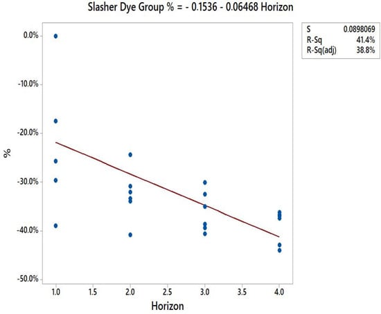
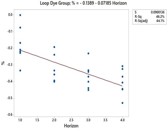
Scheme 2.
Simple Linear Regression.
Therefore, obtained the formulation can be tested in other companies.
Slasher dye:
gain % = −0.1536 − 0.06468 × h
Loop dye:
where: h—planning horizon.
gain % = −0.1389 − 0.07185 × h
5. Conclusions
The present work was limited to bringing science a formulation that can simulate the gain in setup time when comparing the model optimized by the TSP with the empirical model in companies with a similar process. In addition, to prepare the proposal, it was necessary to apply OR, specifically, PI, using the TSP as an approach.
The study brought to light that the influence of the SKU number is not related to the variation in setup time. However, the growth of this number can impact the batch size because the more SKUs is composing the portfolio, the smaller the batch sizes will be, and consequently, more setups will be needed.
The operation has a limitation regarding the dependence of the weaving sector on the dyeing sector. Therefore, to assure the supply of the weaving industry and avoid idleness, the dyeing sector must work in the function of the weaving industry. Therefore, the scheduling optimized proposed can be compromised. Another restriction that impacts the quality of the dyeing sequencing is the limited stock of intermediate rolls between dyeing and weaving, limiting the dyeing flexibility. Depending on the proposed optimized sequencing, there may be a disruption in the weaving supply. In addition to not coinciding with the need for the weaving sector, it may not have an intermediate roll stock that absorbs this mismatch, resulting in machine stoppage. In this way, the programmer will face the tradeoff between dye sequencing and weaving supply.
Moreover, to deal with this problem, it is proposed to discuss the decoupling point. According to [34], the decoupling end refers to the position within the supply chain, where the production flow changes from pushed to pulled, corresponding to the demand penetration point. It is the separation between what is produced for stock and what is produced to order. In this case, it is proposed to shift the decoupling point from the finished product stock (higher added value) to the intermediate stock between the dyeing and weaving sectors (lower added value), increasing the warp roll stock so that the sequencing dyeing does not compromise the supply of the weaving. Consequently, a working capital gain is expected due to the difference in the added value of the two inventories.
The objectives created to carry out this work were pursued. For future research, the study of a model that serves both the dyeing area and the weaving area is also necessary to assess the stock levels and deepen the study of the decoupling point.
It is expected that this work will arouse the interest of textile industries in the use of OR techniques to solve problems in the production process, using mathematical models and software for accurate simulations, allowing a broad view, and contributing to decision making [35].
Supplementary Materials
The following are available online at https://www.mdpi.com/article/10.3390/app11146467/s1, Table S1: Setup time matrix, Machine 7 belonged loop dye group—(minutes).
Author Contributions
Conceptualization, P.R.P. and U.T.G.; Data curation, U.T.G.; Formal analysis, U.T.G. and P.R.P.; Funding acquisition, U.T.G. and P.R.P.; Investigation, R.D.S. and U.T.G.; Methodology, R.D.S. and P.R.P.; Project administration, P.R.P. and U.T.G.; Resources, U.T.G. and R.D.S.; Software, P.R.P.; Supervision, P.R.P.; Validation, R.D.S.; Writing—original draft, U.T.G. and P.R.P. All authors have read and agreed to the published version of the manuscript.
Funding
This research was funded by the National Council for Scientific and Technological Development (CNPq), grant number 304272/2020-5.
Institutional Review Board Statement
Not applicable.
Informed Consent Statement
Not applicable.
Data Availability Statement
Data sharing not appropriate.
Acknowledgments
Plácido Rogério Pinheiro is grateful to the National Council for Scientific and Technological Development (CNPq) for developing this project.
Conflicts of Interest
The author declares no conflict of interest.
References
- Porter, M.E. The Five Competitive Forces That Shape Strategy. Harv. Bus. Rev. 2008, 86, 78. [Google Scholar] [PubMed]
- Jacson, R.H.F.; Jones, A.W.T. An Architecture for Decision Making in the Factory of the Future. Interfaces 1987, 17, 15–28. [Google Scholar] [CrossRef]
- Chiavenato, I. Gestão da Produção: Uma abordagem Introdutória, 3rd ed.; Manole: São Paulo, Brazil, 2017. [Google Scholar]
- ABIT. Perfil do Setor: Dados Gerais do Setor Referentes a 2018 (Updated in 2019). Available online: https://www.abit.org.br/cont/perfil-do-setor (accessed on 11 November 2020).
- Albin, A.M.; Gaudreault, J.; Quimper, C.G. Leverage constraint scheduling: A case study to the textile industry. In Integration of Constraint Programming, Artificial Intelligence, and Operational Research; Springer: Cham, Switzerland, 2020. [Google Scholar]
- Allahverdi, A.; Ng, C.T.; Cheng, T.C.E.; Kovalyov, M.Y. A survey of scheduling problems with setup times or costs. Eur. Oper. Res. 2008, 187, 985–1032. [Google Scholar] [CrossRef] [Green Version]
- Gendreau, M.; Laporte, G.; Guimarães, E.M. A divide and merge heuristic for the multiprocessor scheduling problem with sequence dependent setup times. Eur. J. Oper. Res. 2001, 133, 183–189. [Google Scholar] [CrossRef]
- Paul, R. Denim and jeans: An overview. Denim—Manufacture, Finishing and Applications. In Denim; Elsevier: Amsterdam, The Netherlands, 2015; pp. 1–11. [Google Scholar]
- IEMI. Brasil Têxtil: Relatório Setorial da Indústria Têxtil Brasileira; IEMI: São Paulo, Brazil, 2020; Volume 20. [Google Scholar]
- Zang, R. Sustainable Scheduling of Cloth Production Processes by Multi-Objective Genetic Algorithm with Tabu-Enhanced Local Search. Sustainability 2017, 9, 1754. [Google Scholar] [CrossRef] [Green Version]
- Lima, F.; Ferreira, P. Índigo: Tecnologias, Processos, Tingimento, Acabamento, 1st ed.; Artes Gráficas: Recife, Brazil, 2007. [Google Scholar]
- Li, S.; Cunninghan, A.B.; Fan, R.; Wang, Y. Identity blues: The ethnobotany of the indigo dyeing by Landian Yao (Iu Mien) in Yunnan, Southwest China. J. Ethnobiol. Ethnomedicine 2019, 15, 1–14. [Google Scholar] [CrossRef] [PubMed]
- Guimarães, L.; Klabjan, D.; Almada-Lobo, B. Modeling lot sizing and scheduling problems with sequence dependent setups. Eur. J. Oper. Res. 2014, 239, 644–662. [Google Scholar] [CrossRef]
- Lustosa, L.; Mesquita, M.A.; Oliveira, R.J. Planejamento e Controle da Produção; Elsevier: Rio de Janeiro, Brazil, 2008. [Google Scholar]
- Tubino, D.F. Planejamento e Controle da Produção: Teoria e Prática; Atlas: São Paulo, Brazil, 2007. [Google Scholar]
- Carvalho, R.M. Otimização Bi-Objetivo Para o Problema de Sequenciamento de Tarefas em um Máquina com Tempos de Preparação Dependente da Sequencia. Master’s Thesis, Electrical Engineering, Universidade Estadual de Campinas, Campinas, Brazil, 2002. [Google Scholar]
- Andrade, E.L. Introdução à Pesquisa Operacional: Métodos e Modelos Para Análise de Decisões, 5th ed.; LTC: Rio de Janeiro, Brazil, 2015. [Google Scholar]
- Belfiore, P.; Fávero, L.P. Pesquisa Operacional Para Cursos de Engenharia, 1st ed.; Elsevier: Rio de Janeiro, Brazil, 2013. [Google Scholar]
- Masutti, T.A.; Castro, L.N. A self-organizing neural network using ideas from the imune system to solve the traveling salesman problem. Inf. Sci. 2009, 179, 1454–1468. [Google Scholar] [CrossRef]
- Silva, G.A.N.; Silva, F.A.; Russi, D.T.A.; Pazoti, M.A.; Siscouto, R.A. Algoritmos heurísticos construtivos aplicados ao Problema do Caixeiro Viajante para a definição de rotas otimizadas. Colloq. Exactarum 2013, 5, 30–46. [Google Scholar] [CrossRef]
- Solem, O. Contribution to the solution of sequencing problems in the process industry. Int. J. Prod. Res. 1974, 12, 55–75. [Google Scholar] [CrossRef]
- Desrochers, M.; Laporte, G. Improvements and Extensions to the Miller-Tucker-Zemlin Subtour Elimination Constraints; Elsevier Science Publishers: Amsterdam, The Netherlands, 1991. [Google Scholar]
- Miller, C.; Tucker, A.; Zemlin, R. Integer programming formulations and travelling salesman problems. J. Assoc. Comput. Mach. 1960, 7, 326–329. [Google Scholar] [CrossRef]
- Lakatos, E.M.; Marconi, M.A. Fundamentos de Metodologia Científica, 3rd ed.; Atlas: São Paulo, Brazil, 1991. [Google Scholar]
- Shannon, R.E. Systems Simulation: The Art and Science; Prentice-Hall: Englewood Cliffs, NJ, USA, 1975. [Google Scholar]
- Castro, J.G. A Programação de Lotes Econômicos de Produção (ELSP) com Tempos e Custo de Setup Dependentes da Sequência: Um estudo de caso. Rev. Gestão Industrial. 2005, 1, 60–70. [Google Scholar] [CrossRef]
- Maxwell, W.L. The scheduling of economic lot sizes. Nav. Res. Logist. 1964, 11, 89–124. [Google Scholar] [CrossRef]
- Schrage, L. Optimization Modeling with LINGO; Lindo Systems: Chicago, IL, USA, 2010. [Google Scholar]
- Pinheiro, P.R.; Oliveira, P.R. A Hybrid Approach of Bundle and Benders Applied Large Mixed Linear Integer Problem. J. Appl. Math. 2013, 2013. [Google Scholar] [CrossRef]
- Junior, B.A.; Pinheiro, P.R.; Saraiva, R.D. A Hybrid Methodology for Nesting Irregular Shapes: Case Study on a Textile Industry. IFAC Proc. Vol. 2013, 46, 15–20. [Google Scholar] [CrossRef]
- Pureza, V.; Morabito, R.; Luna, H.P. Modeling and solving the travelling salesman problem with priority prizes. Pesqui. Oper. 2018, 38, 499–522. [Google Scholar] [CrossRef]
- Applegate, D.L.; Bixby, R.E.; Chvátal, V.; Cook, W.J. The Traveling Salesman Problem: A Computational Study; Princeton University Press: Princeton, NJ, USA, 2007. [Google Scholar]
- Triola, M.F. Introdução à Estatística, 7th ed.; LTC: Rio de Janeiro, Brazil, 1998. [Google Scholar]
- Mason-Jones, R.; Towill, D.R. Using the Information Decoupling Point to Improve Supply Chain Performance. Int. J. Logist. Manag. 1999, 10, 13–28. [Google Scholar] [CrossRef] [Green Version]
- Pinheiro, P.R.; Amaro Júnior, B.; Saraiva, R.D. A Random-Key Genetic Algorithm for Solving the Nesting Problem. Int. J. Comput. Integr. Manuf. 2016, 29, 1159–1165. [Google Scholar] [CrossRef]

Publisher’s Note: MDPI stays neutral with regard to jurisdictional claims in published maps and institutional affiliations. |
© 2021 by the authors. Licensee MDPI, Basel, Switzerland. This article is an open access article distributed under the terms and conditions of the Creative Commons Attribution (CC BY) license (https://creativecommons.org/licenses/by/4.0/).