Machine Learning-Based Tools for Wind Turbine Acoustic Monitoring

Abstract

The identification and separation of sound sources has always been a difficult problem for acoustic technicians to tackle. This is due to the considerable complexity of a sound that is made up of many contributions at different frequencies. Each sound has a specific frequency spectrum, but when many sounds overlap it becomes difficult to discriminate between the different contributions. In this case, it can be extremely useful to have a tool that is capable of identifying the operating conditions of an acoustic source. In this study, measurements were made of the noise emitted by a wind turbine in the vicinity of a sensitive receptor. To identify the operating conditions of the wind turbine, average spectral levels in one-third octave bands were used. A model based on a support vector machine (SVM) was developed for the detection of the operating conditions of the wind turbine; then a model based on an artificial neural network was used to compare the performance of both models. The high precision returned by the simulation models supports the adoption of these tools as a support for the acoustic characterization of noise in environments close to wind turbines.

1. Introduction

In recent years, the global energy supply has been characterized by the development of various technologies defined as renewable, which make it possible to obtain energy in a clean and inexhaustible way by exploiting the wind, solar, hydroelectric, and geothermal resources present on Earth. The term “renewable energies” refers to energies that can be regenerated in a short time compared to human history [1]. The sources of these forms of energy are called renewable energy resources. For millennia, wind has represented a form of local energy that can be easily transformed, with examples such as mills and sailing boats illustrating that humans had already recognized its great significance in 2000 BC [2,3].

The machines used to extract energy from wind are wind turbines, ranging from their most archaic forms in ancient mills to the most modern and immense machines with which offshore parks are built, which retain the fundamental characteristic of extracting kinetic energy through blades that rotate around a vertical or horizontal axis [4,5,6]. Turbines can be classified according to two main aspects: aerodynamic operation and construction design. Aerodynamic operation defines the method by which the blades convert airflow into energy. According to this aspect, lift and drag turbines can be distinguished from one another [7,8]. The most common form of turbines are those that use lift; in which, compared to drag turbines, the wind flows on both sides of the blade (which has two different profiles) thus creating a zone of downforce on the upper surface compared to that on the lower surface. The wing profile of the blade leads to different fluid flow velocities on the upper and lower surfaces, which produces the pressure difference [9]. This pressure difference determines a force called aerodynamic lift, similar to that generated on the wings of aircraft. As for turbines based on dragging, they take advantage of the simple aerodynamic pressure that is exerted by the wind impacting the surface of the blades. Finally, classification according to the construction design is based on dividing the turbines into two large groups that are easily distinguishable: turbines with a vertical rotation axis and turbines with a horizontal rotation axis [10].

In the past, the main objective of the use of a wind turbine was to obtain maximum performance, whereas currently, there is a tendency to care about other aspects such as the generated noise, and to include it among the turbine’s specifications [11]. The noise emitted by wind turbines represents one of the most important problems affecting the quality of life of the residents in the vicinity of wind farms, limiting the large-scale diffusion of wind energy. The sound emission produced can be divided into two categories: noise produced by mechanical parts and aerodynamic noise [12]. The greatest contribution to the noise emitted by a wind turbine is attributable to the friction of the air with the blades and the support tower, whereas the modern machinery placed in the nacelle is relatively silent. Aerodynamic noise is caused by the movement of the turbine blades in the air. This motion leads to complex sound generation phenomena, and often, the emission associated with these sources is broadband. Three types of aerodynamic noise can be defined, according to the different mechanisms that cause them. Low-frequency noise is generated when a rotating blade encounters localized flow deficiencies due to the tower, when there is a change in wind speed or the wind spreads between the other blades [13]. Another noise is caused by the turbulent flow, which depends on the increase in atmospheric turbulence that appears as localized forces or pressure variations on the blade. Finally, there is a noise generated by the airfoil, which consists of the sound generated by the flow of air along the surface of the profile. This type of sound is typically broadband, but tonal components can occur due to the smoothing of the edges, or from the action of the airflow on cracks and holes [14].

In evaluating the noise emitted in a residential area, it is essential to identify all the sound sources that contribute to the annoyance caused to residents. Often this procedure is made difficult by the simultaneous contribution of different sources of a different nature which overlap. The acoustic characterization of these sources makes it possible, in some cases, to isolate these contributions, which can thus be removed or added. In this way, it is possible to evaluate the contribution of every single source to the perceived disturbance. When the frequency contributions of different sources overlap, this isolation is no longer possible, at least with the use of classic techniques. In these cases, it becomes essential in the noise disturbance assessment procedure to identify the presence of a specific source within the ambient noise [15].

In recent times, the use of machine learning-based algorithms for the identification of patterns in complex environments has become widespread [16,17,18,19]. At first, these technologies were widely used in the field of computer vision [20,21], but soon proved to be useful for identifying sources in complex sound environments [22,23]. The idea behind the concept of machine learning is to provide computers with the ability to learn and replicate certain operations without having been explicitly programmed. These operations are generally of a predictive or decision-making type and are based on the data available. The machine, therefore, will be able to learn to perform certain tasks by improving, through experience, its skills, responses, and functions. At the basis of machine learning, there are a series of different algorithms that, starting from primitive notions, will process a result. A distinction between the various algorithms is given by the type of learning performed: depending on the training mode, supervised and unsupervised learning can be distinguished. In the first case, the model is trained by providing labeled data as an input, so in addition to the value of the chosen feature, a label with the class to which the data belongs will also be available [24]. On the contrary, to algorithms that exploit unsupervised learning, datasets are given without labels, and it is therefore the program that must find the classes in which to divide the data through features [25]. Then, depending on the different types of task they perform, the algorithms take various names. Classifiers are algorithms that, having input data and the classes to which they belong, can develop a way to understand which class a datum belongs to if they have never seen it before. Another type of algorithm is clustering algorithms, which can divide data taken from inputs without knowing the classes to which they belong. There are also regression algorithms that try to predict the value of data. Using other inputs of the same phenomena, they try to understand their trends by predicting the value of an unknown datum via interpolation [26].

In this study, the measurements of the noise emitted by a wind turbine carried out inside a house were used to develop a classifier capable of discriminating between the operating conditions of the turbine. To do this, a model based on artificial neural networks has been built which uses the sound pressure levels at different frequencies as inputs and returns the operating conditions of the turbine. The article is developed as follows: Section 2 describes in detail the methodologies used in the study: first, the instruments used to carry out the acoustic measurements and the noise detection techniques are described, along with the algorithms used to elaborate the numerical simulation model based on the support vector machine (SVM). In Section 3 the results obtained from the measurements of the noise emitted by the wind turbines and subsequently the results obtained through the numerical simulation are reported and discussed in detail. Finally, Section 4 summarizes the results obtained from this study and discusses possible uses of the technology developed in real cases.

2. Materials and Methods

The wind farm under study is located in a hilly area of southern Italy with an agricultural vocation, where the cultivation of durum wheat, soft wheat, tobacco, sunflower, vegetables, and other minor crops has developed. The presence of tree crops is concentrated in some niches of the territory, and on small or very reduced surfaces (Figure 1).

In this area, there is a wind farm with several wind turbines. The turbines included in this study have a horizontal axis structure with a nominal power of 2 MW [27]. The towers are of a monopolar tubular type, with a hub height of 80 m, equipped with three blades with a diameter of 95 m, made of glass fibers. The maximum power is obtained in a speed range from 10.5 m/s to 25 m/s. Beyond this speed, the blades stop for safety reasons.

Acoustic measurements were carried out to evaluate the noise emissions by the wind turbines under study. The measurements were carried out inside a private house near the wind turbines, with windows open in order to detect the conditions of maximum disturbance. The instrument used for the noise detection was positioned about 1.2 m from the window and placed on a tripod at a height of 1.60 m from the ground. The room where the measurements were made was 3 m high, 4 m long, and 5 m wide, and was normally furnished [28,29,30].

The following instrumentation was used: a LXT1 Larson Davis integrating sound level meter model of “Class 1”, and a Larson Davis CAL 200 Calibrator. The instrumentation used complied with the requirements of the IEC61400-11 standard for wind turbines [31]; the sound level meter was configured for the acquisition of the equivalent level of linear sound pressure, weighted “A”, of the statistical levels with a fast time constant and of the frequency spectra of 1/3 of an octave.

The acoustic measurements were performed in different measurement sessions spread over several days. For every measurement session, measurements were made in different operating conditions of the turbines to assess the contribution made to the sound field by the operation of each wind turbine. The following operating conditions were identified and classified:

• 0 = All turbines off;
• 1 = All turbines on;
• 2 = One turbine off;
• 3 = Two turbines off.

The measured sound levels were compared in order to identify the operating conditions of the wind farm. To do this, the time history and the third-octave frequency spectra of the average and minimum values of the acoustic measurements were analyzed.

The results of the sound level measurements were used as inputs to train a classifier based on the support vector machine algorithm. The classifier will allow us to recognize the operating conditions of the wind turbine, thus providing the technician with the possibility of identifying scenarios in which the sources are turned on/off.

Classification consists of identifying to which category a newly observed datum belongs, based on a set of data known as training data. An algorithm that implements a classification method based on the observations found during training is called a classifier. This term is also used in mathematics to indicate a function, implemented by a classification algorithm, which maps the input data into a category [32]. In the case of support vector machines, classification is considered an instance of supervised learning. Classification is therefore an example of the more general problem of pattern recognition, which consists in assigning some kind of output value to a given input value. To obtain a clearer idea of what the purpose of the classification is, let us consider the case of binary classification and represent the data on a plane. We have N data, also called training points, where each input datum has a D attribute, so it is a vector of dimension D, and belongs to one of the two classes.

The training data depicted in Figure 2 consist of several instances belonging to two different classes. These instances are separable by straight lines, so they are linearly separable. Conversely, when instances of a data collection are not separable by straight lines, they are separable in a non-linear way. The data represented in the plan can appear to us, at this point, as being distributed in two different ways. We may be faced with linearly separable data or non-linearly separable data. In the first case it will be possible to draw in the graph a line (if D = 2) or a hyperplane (if D > 2) that exactly divides the two classes (Figure 2). In the first reported case, we can intuitively draw a straight line dividing the two classes, indicated with the colors blue and red. In the second case it is impossible to draw a line that divides the two classes in half because some points would be found on the wrong side of the separator line [33].

An SVM-based classification technique allows the classification of both linear and non-linear data collections. An SVM represents all instances of the training data collection on a plane consisting of a number of axes (dimensions) equal to the number of attributes that make up the instances. For example, if an instance consists of three attributes, then the training data will be represented on a three-dimensional plane. The three main characteristics of an SVM classifier are: (1) lines or hyperplanes, depending on whether the classifier has a two-dimensional or n-dimensional graph; (2) margins; and (3) support vectors. A line or a hyperplane constitutes a boundary that allows one to classify the instances belonging to different classes by dividing them between the classes. A margin is a distance between the two closest instances of different classes.

Instead, support vectors represent the most difficult instances to classify for an SVM, since they are found within the boundaries of a hyperplane. An SVM allows both the classification of data collections that are linearly separable between the various classes and those of which the instances are separable in a non-linear way. The instances of a data collection are linearly separable if, after having represented them on a plane, they are separable by one or more straight lines.

An SVM is applied differently depending on the type of instances of a collection of data to be classified, whether they are linearly separable or not. In the presence of linearly separable instances, it is necessary to find—among all the straight lines or among all the hyperplanes that separate them between the different classes—those that maximize the margin value. In fact, the line or hyperplane with the maximum margin value is selected since it allows us to minimize the classification error.

Regarding those collections of data that can be separated in a non-linear manner, the classification procedure is more complex, as it is necessary to operate in two separate phases and extend the behavior of the previous approach. In the first phase, the instances of the data collection are mapped to a larger dimensional space in order to make them separable in a linear way. Finally, in the second phase it is possible to use the previous approach to search for a line or a hyperplane that maximizes the size of the margin, since now the instances are linearly separable.

To use the classification through hyperplanes for data that would require non-linear functions to be separated, it is necessary to resort to the technique of feature spaces. This method, which is the basis of SVM theory, consists in mapping the initial data into a space of a higher dimension. Therefore, assuming m > n, for the map we use the function expressed in Equation (1):

$$f:{ \mathrm{R}}^n \to { \mathrm{R}}^m$$

(1)

In Equation (1):

• x and y are input vectors
• f is a transformation function

The technique of image spaces is particularly interesting for algorithms that use training data only through scalar products. In this case, in the space R^m we do not have to find f (x) and f (y) explicitly but it is enough to calculate their scalar product f (x) · f (y). The function f is used to map the input from the n-dimensional space to the m-dimensional space, at a higher level than the n level. To make this last calculation simple—as it becomes very complicated in large spaces—a function called a kernel is used, which directly returns the scalar product of the images (Equation (2)).

$$K \left(x,y\right)=f\left(x\right) ·f\left(y\right)$$

(2)

In Equation (2), the $“·”$ denotes the dot product operation that takes the dot product of the transformed input vectors. The goal of the kernel function is to use the data as an input and transform it into the required form if it is not possible to determine a linearly separable hyperplane, as is the case in most cases [34].

The most used kernels are:

• Linear:

$$K\left(x, y\right)= \mathrm{x} · \mathrm{y}$$

(3)

This is the simplest type of kernel.

• Polynomial:

$$K\left(x, y\right)={\left(\mathrm{x} · \mathrm{y}\right)}^d$$

(4)

This kernel contains a parameter: a degree of freedom d. A d value of 1 represents a linear kernel. A value greater than d will make the decision limit more complex and could lead to data overfitting.

• Radial Basis function (RBF):

$$K\left(x,y\right)= \exp \left(-\frac{{\Vert \mathrm{x} · \mathrm{y}\Vert }^2}{2{\mathsf{\sigma }}^2}\right)$$

(5)

The value of this type of kernel decreases with distance and varies between zero and one; for this reason, it can be considered a measure of similarity.

• Sigmoid:

$$K\left(x, y\right)= \tan \mathrm{h}\left(\mathsf{\alpha } \mathrm{x}·\mathrm{y}-\mathsf{\delta }\right)$$

(6)

There are two adjustable parameters in the sigmoid kernel, the alpha slope and the intercept constant $\mathsf{\delta }$. A common value for alpha is 1/N, where N is the size of the data.

For SVMs, both training and error evaluation are fundamental. For this reason, the data are divided into training and testing sets. The first group is used for algorithm training and contains the correct inputs and outputs, as supervised training is required. It usually consists of about 70% of the total data. The second is used for testing, and consists of a set of data containing 30% of the unused data, that is, to evaluate the accuracy of the neural network by calculating the prediction error chosen. This phase also allows the testing the algorithm; thus, it consists in the real use of the designed model.

One of the advantages of a support vector machine-based classifier is the ability to solve difficult and non-linear classification problems and ensure a high level of classification accuracy. As for solving simple problems, however, the accuracy is comparable to that of a classification technique based on a decision tree. Among the disadvantages are the high model creation time, although it is lower than that used by a neural network, and the non-interpretability of the model.

3. Results and Discussion

The measurements were carried out during May 2018. In the monitoring period, average wind speeds ranging between 9.0 m/s and 23.0 m/s were detected. During the measurements, the turbines were switched on and off according to the sequence shown in

Table 1. Summary of the acoustic measurements carried out in time intervals representative of different operating conditions. The measurements refer to several days of monitoring (Figure 3). 0 = all turbines off, 1 = all turbines on, 2 = one turbine off, 3 = two turbines off.

Operating Condition	Start of Monitoring (Hours)	Monitoring Periods (Hours:Minutes:Seconds)	LeqA (dBA)	Average Wind Speed (m/s)
1	22:00:00	02:00:00	38,4	9.0
2	00:00:00	00:20:00	36,8	9.1
3	00:20:00	00:20:00	31.2	9.2
0	00:40:00	00:20:00	24.9	9.0
1	23:00:00	01:00:00	40.2	13.0
2	00:00:00	00:20:00	38.4	14.0
3	00:20:00	00:20:00	38.5	15.0
0	00:40:00	00:20:00	40.7	17.0
1	01:00:00	02:40:00	50.3	14.0
0	02:40:00	01:50:00	50.8	23.0
1	20:30:00	02:30:00	43.7	12.0
2	00:00:00	00:30:00	42.0	10.8
0	00:30:00	00:30:00	36.7	10.5
1	01:12:00	04:01:00	45.8	10.7

. During the measurements, the following operating conditions were monitored: all turbines off, all turbines on, one turbine off, and two turbines off. The monitoring period covered approximately 18 h of overall measurements. Figure 3 shows the time history of the sound pressure level for the operating conditions performed in the measurement session. The different operating conditions have been highlighted in the following paragraphs to better appreciate the differences in the measured levels from a visual point of view.

Analyzing Figure 3, it is possible to identify the operating conditions indicated above, at least in the first part of the measurements where the wind speed was kept at low levels. This indicates that the source characterizing the background noise is represented by the wind turbine under analysis. The background noise, in fact, undergoes a substantial decrease in the period in which the wind turbine is switched off. It is also possible to verify that under the same operating conditions, the recorded noise changes over time. This fact in the case of turbines in operation can be attributed to the different speeds of the blades, which generate different contributions to the environmental noise. On the contrary, in the conditions with the turbine off, this different trend of background noise confirms that the contributions to the environmental noise have a different origin.

A considerable increase in the noise detected by the instrument can be seen in the central part of Figure 3. By analyzing the measured values of the wind speed in this monitoring period (Table 1) it is possible to verify that these speeds undergo a significant increase. This helps us to understand that the increase in noise is due to the noise of the blades which, turning with greater speed due to the greater energy supplied by the wind, produce greater noise. However, analyzing the final part of the monitoring where all the turbines have been turned off, we can see that the background noise with the turbines off is much greater than that recorded in the initial part of the monitoring. This confirms the essential contribution of sources other than wind turbines to the background noise. Among these, the noise of the wind demonstrates a significant weight, impacting on trees or buildings and on the pavement and thus contributing to the background noise.

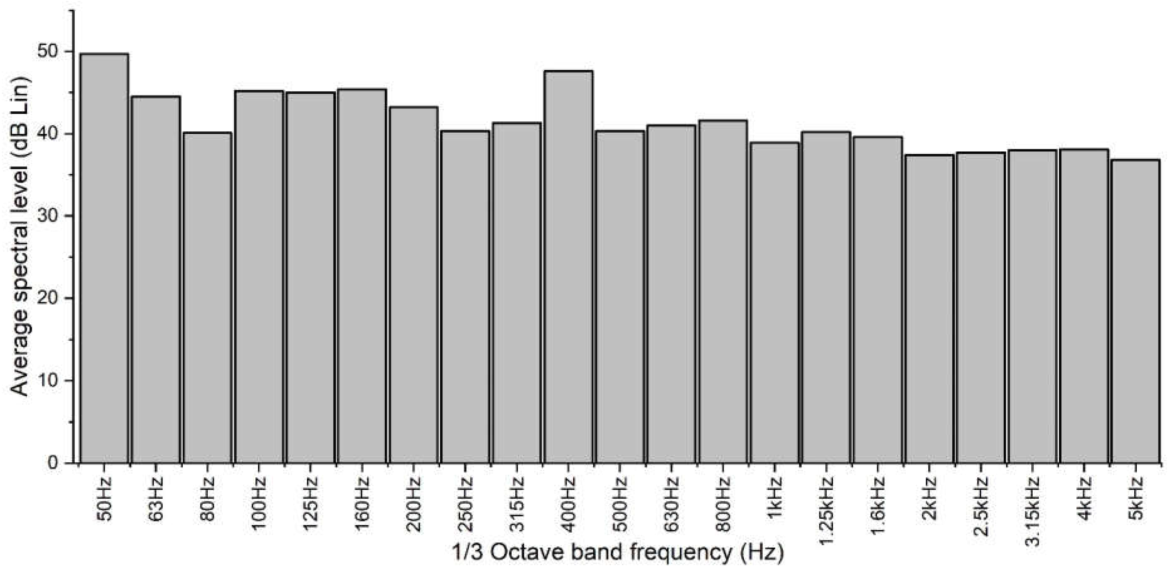
Figure 4 shows the average spectral levels in the one-third octave bands between 50 Hz and 5 kHz for the entire measurement session.

From the analysis of Figure 4, it is not possible to obtain useful information to characterize the sources. The noise is distributed over the entire frequency range, with values ranging from 40 dB to about 50 dB. There are no tonal components that can identify a specific source. In order to extract further information, it is necessary to individually analyze the portions of measurements relating to the various operating conditions.

The results of the measurements were subsequently elaborated in order to look for the characteristics that were able to discriminate between the different operating conditions of the wind turbines. According to the analysis of Figure 3, fourteen periods were identified (Table 1). Table 1 shows the durations and the acoustic measurements for the operating conditions performed in the measurement session. Based on the analysis of the results, it is possible to note that the different operating conditions are confirmed by the noise levels recorded by the sound level meter. The operating conditions with the turbines on returned the following values: 38.4, 40.2, 50.3, 43.7, and 45.8 dBA. The operating conditions with the turbines off, however, returned the following values: 24.9, 40.7, 50.8, and 36.7 dBA. These results show that the extreme operating conditions recorded noise values conditioned by the wind speed, demonstrating that the contribution of the wind to the background noise became significant under certain circumstances.

The selected periods do not show anomalous or occasional phenomena. Therefore, they can be used for setting the classification model. To build a classification model of the operating conditions of the wind turbine, the measured data were resampled by setting 1 s as the integration time. For each observation, the A-weighted equivalent sound pressure levels for each one-third octave band were calculated. 64,860 observations were collected, and 21 variables were selected. To characterize the three periods, we decided to use the average spectral levels in one-third octave bands between 50 Hz and 5 kHz as descriptors.

Figure 5 shows the average spectral levels in the third-octave bands between 50 Hz and 5 kHz for some of the observation periods identified. To facilitate the comparison, the periods of operation of the turbines have been placed side by side with periods of inactivity. From the analysis of the results shown in Figure 5, it is possible to note that the operating conditions are not easily identifiable. We can see that the conditions in which the turbines are switched off have lower values at high frequencies. However, not all frequencies contribute to the identification of the operating conditions. This indicates that not all frequencies are required for the model setup.

Analyzing the information contained in Table 1, we can confirm that in the four monitoring periods shown in Figure 5, the wind conditions remained almost constant. In fact, in all four measurements the wind speed remained approximately equal to 9.0 m/s (9.0–9.2). These boundary conditions allow us to be able to make a comparison between the different operating conditions of the wind farm. Figure 5a shows the average spectrum detected with all turbines on. A considerable energy contribution can be appreciated at both low and medium frequencies, with peaks recorded at 50 Hz and 125 Hz. The operating conditions with all turbines on showed the highest spectral values. Figure 5b shows the average spectrum detected with only one turbine off; in this case the energy contribution was also considerable, and no large differences were detected, at least through a visual analysis of the large differences with the operating conditions with all turbines on. Furthermore, there were peaks corresponding to the frequencies at 50 Hz and 125 Hz, but these showed lower values. Figure 5c shows the average spectrum detected with two turbines off; in this operating condition the energy contribution was significantly reduced. Once again, a peak at 50 Hz was recorded, although it was of a lower value, as well as a second peak at 200 Hz. Finally, Figure 5d shows the average spectrum detected with all turbines off; in this case, the energy contribution measured by the instrument was significantly decreased compared to the case where all turbines were on. Furthermore, it is possible to note that a peak at 50 Hz was confirmed, whereas the contribution to the medium frequencies that was recorded in the other three operating conditions was completely absent.

In addition to the extreme frequencies that have already been excluded from our analysis—having considered only the frequencies between 50 Hz and 5 Khz—there may be other frequencies that are not essential for the correct identification of the operating conditions. To identify the characteristics that are able to discriminate between the different operating conditions, a visual analysis was conducted through a wrapper for density lattice plots (Figure 6).

The bell curves show the distribution set at each frequency for the four identified operating conditions. As already indicated, extreme frequencies were left out of this analysis, which focused on the frequency range between 50 Hz and 5 kHz. In this frequency range, it can be observed that some discriminate these other labeled operating conditions better than others. For these components, it can be noted that the four operating conditions assume different distributions, but these are not easily identifiable, at least not with a purely visual approach. This is because in all cases the distributions overlap; this indicates that in these ranges of values it is not possible to use this feature to identify the operating conditions of the turbine. For other components, the distributions appear sufficiently distinct; this suggests that in these ranges of values it is possible to use this feature to identify the operating conditions of the wind farm.

To identify the components that best discriminate the four classification labels, a feature selection procedure was performed to identify which variables are most relevant to the model’s performance. The purpose of selecting features is to find features that allow researchers to better discriminate between different objects, and which are insensitive to translation, rotation, or scale problems. In other words, a reduction in predictors is applied, which reduces the complexity of the information to be processed and makes the system more efficient.

The Boruta algorithm iteratively compares the contribution of each feature to the final classification, with those of features created by randomly mixing the original ones (shadow features). Attributes that prove to be worse than shadow ones are progressively eliminated. Attributes that are significantly better than shadows are confirmed. Shadow features are recreated in each iteration. The algorithm stops when only confirmed attributes remain or when the maximum number of feature selection operations is reached. The purpose of this procedure is to select a subset of predictors from the starting one, which, while reducing the size (columns) of the dataset that retains the initial information, identified the most significant predictors compared to the others [35,36,37].

In

Table 2. Attribute statistics of the feature selection analysis related to the importance of the one-third frequency components, sorted by mean value (Figure 7).

Frequency	Mean	Median	Min	Max
63	79.75986	78.79704	75.02274	86.74699
80	52.25725	52.61418	48.52443	55.3532
400	48.57361	49.25013	45.04599	49.92336
1250	48.5529	48.49379	45.88256	50.25572
5000	48.43594	48.02526	46.85551	52.15254
630	48.17461	48.27758	45.31751	51.56099
125	46.91648	46.98903	44.89291	49.44468
1600	46.69345	46.44566	45.23813	49.22559
50	46.6604	46.30567	44.2554	50.58229
250	46.5574	46.69396	42.49567	49.51197
200	42.81196	42.24069	40.78648	46.74624
4000	40.64552	40.18109	38.25214	42.71576
3150	39.20864	39.28436	36.42129	41.18301
2000	37.03489	37.02878	35.63938	38.51441
500	36.5802	36.46276	35.34557	38.1025
315	36.50848	36.39801	34.21329	38.94105
2500	36.26733	36.34724	34.26245	37.75657
800	36.18964	36.50876	34.22224	38.27648
1000	33.56291	33.53768	31.19339	35.67666
100	33.14273	32.90384	30.52556	35.53637
160	28.65536	28.72809	27.06356	30.34784

, for each feature contained in the data frame, the mean, median, maximal, and minimal importance of the one-third frequency components are shown.

To facilitate the identification of the components that contribute the most to the discrimination between the operating conditions, in Table 2 the results have been sorted in descending order starting from the top (mean value). In this sorting, the column that shows the average value of importance, determined by the selection of characteristics, was used. It can be seen that for the first three components in the frequency range from 63 Hz to 400 Hz, the average of the importance of the variable is greater than 48. This indicates that these characteristics are the ones that provide the greatest contribution to the discrimination between operating conditions.

To obtain an overview and to better appreciate the results, a diagram is presented in Figure 7. Analyzing Figure 7 and Table 2, we can easily identify the variables that recorded the highest values of importance. If the first 10 returned variables (average > 46) are evaluated, it can be seen that they are within the 63-1600 Hz frequency range, with the addition of the 5 kHz frequency. To further reduce the calculation cost and avoid overfitting, we decided to further reduce the number of features selected to take only the first 10 among those that recorded the highest values on average.

The variables selected by Boruta’s method represent the input variables for a support vector machine-based model implemented to detect the operating conditions of the wind turbines. This model creates an SVM classifier to classify the wind turbine operating conditions.

The following SVM architecture was implemented:

• Input data: The first 10 one-third frequency components returned by the feature selection method;
• Radial basis function (RBF) kernel;
• Multiclass classification (four classes).

In the training phase, the algorithms based on SVMs use labeled data; therefore a correspondence between the input values and the relative output values associated with them can be established. In our case, each occurrence related to a combination of one-third frequency components was associated with a value of the relative class. The training aims to identify a set of weights w, one for each characteristic, of which the linear combination predicts the value of the class. This discourse of weight regulation is common with the training of algorithms based on artificial neural networks. Compared to artificial neural networks in SVMs, the optimization of margin maximization is adopted in order to reduce the number of non-zero weights. The results obtained in this way correspond to the characteristics that count in the separation of classes through the identification of a hyperplane. These non-zero weights correspond to the support vectors because they identify the separation hyperplane [38,39].

Before proceeding with the model training, it is necessary to split the data. The sampling methodology used for the subdivision of data can have a significant effect on the quality of the subsets used for training and testing. Poor data splitting can result in inaccurate and highly variable model performance [40]. To evaluate the generalization capacity of the model, the data were divided into two randomly selected groups:

• A training set equal to 70% of the available observations (45,402 samples). These records are used in the training phase to adjust the connection weights through an iterative procedure aimed at minimizing the classification error.
• A test set equal to the remaining 30% of the available observations (19,458 samples). These records are used in the testing phase to evaluate the performance of the numerical simulation model. These are data that the model has never seen before, so they represent a test for the model.

In

Table 3. Confusion matrix for the support vector machine-based model.

	Predictions
Target	0	1	2	3
0	3120	48	31	41
1	787	13,371	61	19
2	14	356	805	85
3	119	24	7	570

, a confusion matrix of the model is shown. The confusion matrix represents a valid tool for assessing the quality of the output returned by a classifier on the data set submitted as the input. The diagonal elements represent the number of points for which the expected label is equal to the true label, whereas the off-diagonal elements are those erroneously labeled by the classifier. The higher the diagonal values of the confusion matrix, the better the performance of the model, thus indicating many correct predictions.

The confusion matrix returned excellent results. The accuracy of the model was high (accuracy = 0.918), confirming that the model can identify the operating conditions of a wind turbine farm. From the analysis of Table 3, it can be verified that the model was able to correctly identify 17,866 observations out of 19,458. To complete the analysis of the results it is appropriate to evaluate how the forecast errors committed by the model were distributed. It can be seen that most errors involved the extreme classes, 0 (all towers off) and 1 (all towers on). Specifically, the model ranked 787 occurrences as 0 when the data were labeled as 1 (probably because wind noise in particular conditions becomes comparable with that produced by wind turbines). Furthermore, it classified 356 occurrences as 1 when instead the data were labeled as 2. This error may be due to the fact that the operating conditions 1 and 2 were very close, since in both these conditions only one turbine was missing. Of the errors mentioned, the first one has a greater weight, as a forecast of non-operation of the turbines when they are all in operation represents a situation that can lead to greater problems. In order to reduce these classification errors, it will be necessary to insert into the model the information related to the wind speeds detected during the monitoring phase.

To compare the classification results obtained using an SVM-based algorithm, the same labeled data were used to train a model based on artificial neural networks (ANNs). ANNs are a family of machine learning techniques composed of layers of interconnected neurons, with an architecture like that of biological neurons [41]. The functioning of an ANN mirrors that of the brain, based on several interconnected neurons working in parallel, which process an input, producing an output that will be sent to subsequent neurons. A very interesting aspect of the functioning of the brain is its ability to continuously vary the weights of the interconnections, making it possible to classify and generalize the stimuli received from the outside. In this way, it promotes adaptation by learning from past signals and consequently trains the model to facilitate learning by allowing new data to be processed more quickly and correctly [42,43].

A neural network is therefore a set of nodes arranged in layers, connected to each other by weights. The first layer is called the input layer and the last is the output layer, whereas the intermediate ones are defined as hidden layers, and are not accessible from the outside as all the characteristics of the complete network are stored in the matrices that define the weights [44,45]. The type of network determines the type of connections that are present between the nodes of different layers and between those of the same layer. The choice of the activation function determines the substantial difference with the corresponding biological neuron. In the latter, the sum of the incoming impulses is transmitted directly to the axons if the threshold is exceeded, essentially behaving like a linear regression model, approximating the distribution of data with a straight line. On the contrary, the use of a non-linear function allows for a better representation of the signals, without considering the fact that sometimes a linear regression is not usable [46,47].

The classifier was developed based on a feed-forward artificial multilayer neural network, with a single hidden layer and a multiclass output that returned the four operating conditions. Feedforward networks are those with the simplest architecture [48,49], being composed of an input layer, one or more hidden layers, and an output layer. Each neuron has its input parameters from the previous layer and no cross-connections are possible between nodes of the same layer or cycles in which the output is sent to previous layers. The flow of information then proceeds in only one direction and the output of each cycle is determined only by the current input. The softmax activation function is used with multinomial cross-entropy as the cost function [50,51,52,53].

Table 4. Confusion matrix for the artificial neural network-based model.

	Predictions
Target	0	1	2	3
0	3015	148	30	47
1	694	13,450	89	5
2	49	291	853	67
3	168	12	14	526

shows the classification results returned by the ANN-based classifier. It can be verified that the model was able to correctly identify 17,844 observations out of 19,458. The accuracy of the artificial neural network-based model was 0.917. We can see that most errors involved extreme the classes, 0 (all towers off) and 1 (all towers on). Specifically, the model ranked 694 occurrences as 0 when the data were labeled as 1, probably for the same reason as that in the SVM model, since wind noise in certain conditions is similar to that produced by wind turbines. It also classified 291 occurrences as 1 when the data were instead labeled as 2. This error may be because operating conditions 1 and 2 were very similar, since in both conditions only one turbine was not working.

Comparing the classification results obtained using an SVM-based algorithm and an ANN-based algorithm (

Table 5. Comparison between the accuracy returned by the SVM-based model and the ANN-based model.

	SVM-Based Model	ANN-Based Model
Accuracy	0.918	0.917

), it appears that the two models provide comparable results, with a slight advantage observed in the SVM-based model.

The effect of the wind on the noise detected in the site of interest is strongly influenced by both the wind speed and its direction. The roughness of the ground exerts a great influence on the wind. The average wind speed decreases because of the ground, but at the same time the wind becomes turbulent. Atmospheric wind is a multi-correlated stochastic process in space and time. The average wind speed, due to the friction exerted by the ground, increases with height, according to an exponential or logarithmic profile. The type of soil therefore affects this profile in such a complex way that it is difficult to quantify the effect exactly. When the wind arrives in the vicinity of the building, noise is generated due to various physical phenomena (airborne noises, mechanical noises, structure-borne noises, and the Eigenmode excitation of elements). These contributions are added to those derived from the noise generated by wind turbines contributing to the background noise. The contribution derived from the wind can in some cases become comparable with that produced by wind turbines when the wind speed increases significantly; however, it is a broadband contribution. The wind direction also influences the contribution to the background noise, both in terms of noise produced by the turbines—which is propagated more effectively when the wind direction is in favor of the site of interest—and in the contribution generated by the impacts of the wind on the elements present in the vicinity of the building. To evaluate these contributions, it is necessary to carry out measurements of the speed and direction of the wind both in the vicinity of the turbine and in the vicinity of the site of interest.

4. Conclusions

The characterization of acoustic sources that contribute to ambient noise has long been a topic of study by researchers around the world. The difficulty in isolating a specific source is due to the considerable complexity of a sound made up of many contributions characterized by spectra of different frequencies. Each sound has a specific frequency spectrum, but when the spectra of different sources overlap it becomes difficult to distinguish between the different contributions. The availability of a tool that is capable of classifying the operating conditions of a wind farm could provide valid support in evaluating the contributions derived from various sources.

Nowadays, machine learning algorithms are widely used in various fields. In many cases, these algorithms have been used to address various problems related to wind turbines. In this study, measurements were mode of the noise emitted by wind turbines. The average spectral levels in the one-third octave bands were visually analyzed in order to identify the frequency range that was capable of discriminating between the operating conditions. A model was then adapted to evaluate the importance of variables in classifying wind turbine functioning classes. To reduce the number of predictor variables, a feature selection analysis was carried out based on the Boruta algorithm. In this way, only the most significant predictors were selected, which were capable of returning a response as close as possible to the expected one. Finally, machine learning-based models were developed, which analyzed the operating conditions of the wind turbine based on the sound pressure level values at specific frequencies. The high accuracy of the SVM model (accuracy = 0.918) suggests that the adoption of this tool could support the acoustic characterization of noise in environments close to wind turbines. Furthermore, the performance shown by the classifier led us to think that this technology could also be used in other fields. In addition, the classification errors committed by the model can be significantly reduced by adding the wind speeds detected during the monitoring phase to the system inputs, so the current model can be improved. This activity will be performed in future studies.