Topological Navigation and Localization in Tunnels—Application to Autonomous Load-Haul-Dump Vehicles Operating in Underground Mines

Abstract

Mobile robots are no longer used exclusively in research laboratories and indoor controlled environments, but are now also used in dynamic industrial environments, including outdoor sites. Mining is one industry where robots and autonomous vehicles are increasingly used to increase the safety of the workers, as well as to augment the productivity, efficiency, and predictability of the processes. Since autonomous vehicles navigate inside tunnels in underground mines, this kind of navigation has different precision requirements than navigating in an open environment. When driving inside tunnels, it is not relevant to have accurate self-localization, but it is necessary for autonomous vehicles to be able to move safely through the tunnel and to make appropriate decisions at its intersections and access points in the tunnel. To address these needs, a topological navigation system for mining vehicles operating in tunnels is proposed and validated in this paper. This system was specially designed to be used by Load-Haul-Dump (LHD) vehicles, also known as scoop trams, operating in underground mines. In addition, a localization system, specifically designed to be used with the topological navigation system and its associated topological map, is also proposed. The proposed topological navigation and localization systems were validated using a commercial LHD during several months at a copper sub-level stoping mine located in the Coquimbo Region in the northern part of Chile. An important aspect to be addressed when working with heavy-duty machinery, such as LHDs, is the way in which automation systems are developed and tested. For this reason, the development and testing methodology, which includes the use of simulators, scale-models of LHDs, validation, and testing using a commercial LHD in test-fields, and its final validation in a mine, are described.

1. Introduction

The development of robotic applications has increased significantly in the last decade, and currently, robotic systems are being utilized for many purposes, in various environments. Mobile robots are no longer used exclusively in research laboratories and indoor controlled environments, but are now also used in dynamic industrial environments and outdoor sites. Moreover, the efforts for developing autonomous cars and drones have had the effect of strengthening the development and use of other autonomous machines and vehicles in various industries.

Mining is one industry in which autonomous vehicles have been in use for at least 13 years. Industrial use of autonomous hauling trucks started in 2008 in the Gabriela Mistral copper open-pit mine, located in the north of Chile. Currently, the use of autonomous mining equipment, mainly vehicles, is an important requirement in the whole mining industry. This is because mining operations need to increase the safety of the workers, as well as to augment the productivity, efficiency, and predictability of the processes. Safety is, without doubt, a key factor, and has been the top priority of mining companies in recent years. This is true, especially, in underground mining operations with their hazardous environments in which workers are constantly exposed to the risks of rock falls, rock bursts, and mud rushes, and where the presence of dust in the air can result in a number of associated occupational diseases in the workers [1].

In an underground mine, autonomous vehicles navigate inside tunnels. This kind of navigation has different precision requirements from those where they are navigating in an open environment. First, tunnels are GNSS-denied environments and thus vehicles cannot use any GNSSs (Global Navigation Satellite Systems) to self-localize. Secondly, when driving inside tunnels, it is not relevant to have an accurate localization system, but it is essential to be able to move safely through the tunnel, and to make appropriate decisions at its intersections and access points. This is completely different from most robotic applications, where safe navigation requires an accurate determination of the robot’s position and orientation at every moment.

To address this need, a topological navigation system for mining vehicles operating in tunnels is proposed and validated in this paper. This system was specially designed to be used by Load-Haul-Dump (LHD) vehicles, also known as scoop trams, operating in underground mines. An LHD is a four-wheeled, center-articulated vehicle with a frontal bucket used to load and transport ore on the production levels of an underground mine (See Figure 1). These machines are a key component in the extraction of ore from underground mines because the ore extraction rate from the mine depends directly on the efficiency of the LHD. The proposed system permits a commercial LHD, which is a very large vehicle, to navigate inside tunnels that are just a couple of meters wider than the LHD. In addition, it allows bi-directional navigation and so-called inversion maneuvers, both required in standard LHD operations inside productive sectors of underground mines. (See an example in Figure 2). In addition, a localization system, specifically designed to be used with the topological navigation system and its associated topological map, is also proposed.

An important aspect to be addressed when working with heavy-duty machinery, such as the LHDs, is the way in which automation systems are developed and tested. In order to address this important issue, we use a development process for autonomous systems for mining equipment, which is comprised of the following four-stages: (i) development using specific simulation tools, which are fed with real data from mining environments, (ii) development using scale-models of the actual machines, (iii) validation and testing using real machines in test-fields, and (iv) validation and testing using real machines in actual mine operations. This development process was used for achieving autonomous navigation of LHDs. The proposed topological navigation and location systems were validated using a commercial LHD, during several months at a medium-scale sub-level stoping mine, located in the Coquimbo Region of Chile.

The main contributions of this paper are the following:

• A topological navigation system for mining vehicles operating in tunnels, which can be used in any tunnel network by any articulated vehicle.
• A novel localization system specifically designed for tunnel-like environments, which estimates the vehicle’s global and local pose using the topological map.
• A development and testing methodology that can be used in the development process of heavy-duty machinery.
• Full-scale navigation experiments using a commercial LHD on a productive level of a sublevel stoping mine.

This paper is organized as follows: First, related work on autonomous LHD navigation is presented in Section 2. The proposed topological navigation system for LHD is described in Section 3. Then, in Section 4, the development and testing methodology is described, and in Section 5, validation results achieved in an actual mine are presented. Finally, conclusions of this work are drawn in Section 6.

2. Related Work

Autonomous navigation of LHDs has been a subject of scientific research since the late 1990s [2,3,4]. The main objectives have been to improve productivity and increase safety for the personnel, but simultaneously to benefit from reduced machine maintenance due to less wear of components. The theoretical development, and experimental evaluation, of a navigation system for an autonomous articulated vehicle is described in [4]. This system is based on the results obtained during extensive in-situ field trials and showed the relevance of wheel-slip for the navigation of center-articulated machines. In [5], one of the earlier industrial automation implementations is reviewed. It is mentioned there, that the use of automation in day-to-day operations offers flexibility and convenience for the operators. The development of what would become the first commercially available solutions for autonomous navigation of LHD machines followed shortly thereafter.

The work of Mäkelä [6] set the basis for the AutoMine software of the LHD manufacturer Sandvik, while the work of Duff, Roberts, and Corke [7,8,9] set a similar precedent for the software MINEGEM of Caterpillar. Only a few years later, the work by Marshall, Barfoot, and Larsson [10,11,12] configured what would become Scooptram Automation of the company Atlas Copco (now Epiroc). These companies have applied their automation solutions directly to their articulated vehicles [13]. Because of their commercial application, only the initial work on the development of the autonomous systems from LHD manufacturers is available in the literature. For instance, autonomous navigation from the manufacturer Sandvik is based on an absolute localization paradigm, i.e., it relies on odometry and detection of natural markers of the tunnel network [6]. Localization is achieved by taking a profile of the tunnel in a 5 [m] long section and comparing it to a known map. Caterpillar, on the other hand, initially based its system on mainly reactive techniques (wall following), in conjunction with a topological map with information about loading points, dump points, intersections, and other markers that are used in an opportunistic location scheme [9]. Finally, Epiroc made use of a hybrid navigation paradigm [11]. A set of behaviors was programmed under a fuzzy logic scheme to form the reactive part, while a higher level (deliberative) planner was used at intersections or open spaces.

Despite its success in delivering a product to market, research in autonomous navigation for underground tunnels continues to be a relevant topic. In [14], a review is given on the performance of automated LHDs in mining operations. It also mentions some issues and challenges that remain. The dynamic and highly variable nature of mining operations underlines the need for flexible and quickly deployable systems, features that earlier commercial solutions lacked [15,16]. These shortcomings are also known to LHD manufacturers, who continue to improve their systems [17].

Automation in mining is, most certainly, a widespread trend that has already shown corporate benefits, and it will continue to drive the modernization of the mining industry [18]. Cost, productivity, and safety are still the driving forces for investments in automated systems. Recent publications in the field also suggest the increasing interest of China in the application of automation technologies [19,20,21]. Particular attention has been paid to modeling, and control techniques.

The autonomous navigation system presented in this paper is based on topological navigation, and model predictive control (MPC). Underground mining environments have been shown to be suited for the extraction of features needed to build topological maps [22], and a mixture of topological and metric maps has been used successfully to map and navigate in large environments [23]. MPC has also been proven to perform well in the high-speed control of vehicles with nonlinear kinematics [24,25,26].

3. Topological Navigation and Localization for LHD

3.1. General System Overview

LHD are large vehicles used in underground mining. In this work a LHD model LF-11H, from the GHH Fahrzeuge manufacturer, is used. The vehicle’s size is 9.71 [m] in length, 2.45 [m] in width, and 2.45 [m] in height. The LHD’s navigation is based on the data provided by two laser scanners (2D LIDARs), one pointing towards the front of the machine, and the other pointing towards the back. For supervision and occasional teleoperation, two cameras give the front and back images to the control station [27]. All on-board processing is done on an industrial computer running Linux OS, while the direct machine control is handled by an internal PLC unit. The LHD and the hardware components mentioned above can be seen in Figure 1.

In order to navigate autonomously inside the network of tunnels of an underground mine a proper representation of the mine is required, in this case a navigation map that includes the topological structure of the mine, tunnels, and intersection, as well as LIDAR measurements. The LHD, therefore, builds a map of the operation area during the system setup, using measurements from LIDAR sensors, as it navigates the tunnels. This map is then linked to a topological representation, thus giving names to all the relevant locations, henceforth referred to as “nodes”. The map, once built, allows for route planning and self-localization of the machine. The latter is carried out by means of scan matching between current LIDAR measurements and the LIDAR landmarks stored in the map. The scan matching is implemented using the ICP (Iterative Closest Point) algorithm, and the final pose estimation is the result of applying a Kalman Filter.

Every time a new mission in which the LHD is requested to move to a target node in the mine is executed, a topological route composed of nodes is defined, and then target poses inside each node are calculated. Afterwards, the path required to reach each target pose is computed, and a reactive control algorithm is put in charge of following the path, keeping the vehicle away from colliding with the walls of the tunnel. A model predictive control strategy is implemented because of the complexity of following the path with this articulated machine, which normally moves at a speed of between 12 and 24 km per hour inside the mine.

3.2. Topological Map and Physical Representation

The main component of the representation of the mine is the “Topological Map” (TM). Two types of nodes are defined on this map: (i) tunnel nodes and (ii) intersection nodes. A tunnel node is a section of the mine that can be traversed back and forth, i.e., it corresponds to a single path or trajectory between two physical points. Topologically, a tunnel node has two edges, connecting it with two intersection nodes. An intersection node may have multiple edges that connect it to other nodes, and it can also traverse back and forth. An example would be a fork in the tunnel, where the vehicle must choose one of the possible path alternatives.

Each topological node contains a number of access points (APs) and waypoints (WPs), which are represented by a 2D pose within the node’s coordinate system. APs connect different topological nodes; they signal the transitions between map nodes. WPs, on the other hand, correspond to specific poses within the topological node, each one containing relevant information for the navigation system, such as maximum driving speed. Examples of waypoints can be a location for dumping ore, a place to park the vehicle, or a location the vehicle must go through when traversing the node.

As an example, Figure 3 shows a portion of a real mine, where a TM has been created. In this scenario, four main tunnels, T6, T7, T9, and T10, and one intersection, I0 (in green), define the map. It can also be seen that T9 contains a number of waypoints throughout its path, shown by arrows.

Besides their associated 2D pose, APs and WPs have a defined heading. APs always face the outer side of the node they are in, but WPs always face in the predefined direction of the node. Because of this, APs and WPs can be connected in 4 different ways: front-to-front, front-to-back, back-to-front, and back-to-back (see Figure 4, the orange arrow is the default direction of the node). In Figure 5, a TM with 2 tunnel nodes, 1 intersection node, and its AP, WP, and the connections between them, is shown.

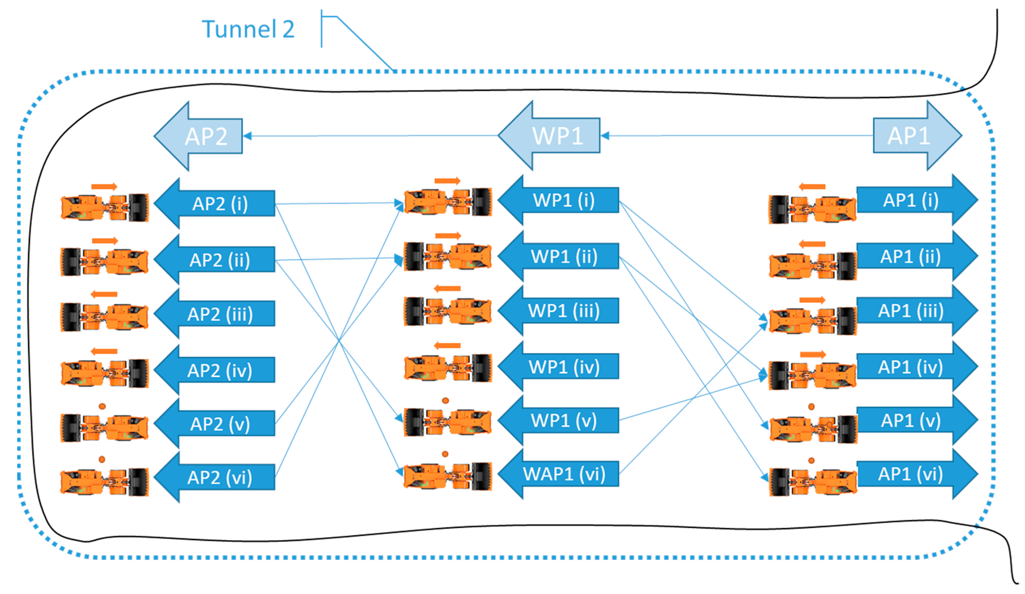
One of the problems that articulated vehicles face while traversing an underground mine is that they sometimes need to change their direction of movement, using a maneuver known as inversion. (See Figure 2). To tackle this problem, a Topological Movement’s Map (TMM) is built automatically from the TM. To do this, for each AP and each WP in the TM, 6 nodes are created in the TMM. These 6 nodes represent how the vehicle would move through an AP or WP in the TM:

(i)

Vehicle going towards the AP/WP moving forward (bucket facing the AP/WP).

(ii)

Vehicle going towards the AP/WP moving backwards (rear bumper facing the AP/WP).

(iii)

Vehicle going away from the AP/WP moving forward.

(iv)

Vehicle going away from the AP/WP moving backwards.

(v)

Vehicle standing on the AP/WP facing in its same direction.

(vi)

Vehicle standing on the AP/WP facing in its opposite direction.

These new nodes in the TMM are then connected using the information on the topological map and a predefined set of rules that reflect how a vehicle would move between two different pairs of nodes in the TM. These rules are presented on

Table 1. TMM’s connection rules for connections within the same TM node.

Origin Node’s Type	Destiny Node’s Type of Connection for Different AP/WP Connection Types
	Front-to-Front	Front-to-Back	Back-to-Front	Back-to-Back
	(i)	-	-	(i) & (vi)	(iii) & (v)
	(ii)	-	-	(ii) & (v)	(iv) & (vi)
(iii)	(i) & (vi)	(iii) & (v)	-	-
(iv)	(ii) & (v)	(iv) & (vi)	-	-
(v)	(i)	(iii)	(i)	(iv)
(vi)	(ii)	(iv)	(ii)	(iii)

and

Table 2. TMM’s connection rules for connections between different TM nodes.

Origin Node’s Type	Destiny Node’s Type of Connection for Different AP/WP Connection Types
	Front-to-Front	Front-to-Back	Back-to-Front	Back-to-Back
(i)	-	-	(i) & (vi)	(iii) & (v)
(ii)	-	-	(ii) & (v)	(iv) & (vi)
(iii)	(i) & (vi)	(iii) & (v)	-	-
(iv)	(ii) & (v)	(iv) & (vi)	-	-
(v)	(i) & (vi)	(iii) & (v)	(i) & (vi)	(iv) & (vi)
(vi)	(ii) & (v)	(iv) & (vi)	(ii) & (v)	(iii) & (v)

. Rules are slightly different when considering the special case of connecting APs from different TM nodes (see Table 2), because as these APs connect different TM nodes, they have the same physical location, and then connections between “stopped” nodes must be allowed.

It is important to note that these connections are directional, and it is required to go through a “stopped” node ((v) or (vi)) to change the vehicle’s direction of movement. Therefore, these rules must be applied in both directions of each connection. Nodes (v) and (vi), with the same origin AP/WP, are always connected. An example of the TMM creation from the TM of Tunnel 1 (in Figure 5) is shown in Figure 6 and Figure 7. For clarity of purpose, only half of the connections are shown in each figure. In Figure 6, only connections in the direction of the tunnel are shown, while in Figure 7, only connections against the direction of the tunnel are shown. Each node in the TMM is represented by a blue arrow. Each node has an associated LHD heading and movement direction. The heading is represented by the LHD image and the movement direction by the orange arrow next to the LHD.

An example is shown in Figure 8 for the inversion maneuver. Relevant TMM nodes involved in the inversion movement are highlighted.

Once the TMM is set up, topological paths can be calculated upon demand. When a new request is received, the vehicle’s current state is pushed to the TMM as a starting point, and then the optimal route to the desired destination is calculated using Dijkstra’s algorithm [28]. Traveling costs between TMM nodes are set up initially based on the distance between AP/WP, but can be fined-tuned with additional considerations such as: the change in the vehicle’s movement direction, the feasibility of the movement (sometimes a curve is too sharp for the vehicle to turn in a certain direction), and unwanted paths for other reasons such as road repairs, narrow spaces, or uneven tracks.

Path planning using the TMM is extremely fast. Its execution in a very large mine layout was simulated in a layout similar to that of the new Chuquicamata underground mine, with eight parallel streets, each one having 19 intersections. Under these conditions, the TMM contained 5378 nodes and 8760 vertices, and path planning using the TMM took less than 5 [ms] on an i7 Intel processor [27].

Each node contains so-called LIDAR-landmarks that are stored when the map is built, and are used for the LHD self-localization. In regard to tunnel nodes, the LIDAR-landmarks correspond to LIDAR point clouds acquired at certain selected positions of the tunnel. In the case of intersection nodes, the LIDAR-landmark corresponds to an integration of the point clouds acquired inside the intersection.

Map Building—Determination of LIDAR-Landmarks

For map building the LHD needs to visit all the tunnels of the mine in one direction. In order to achieve this, the LHD is teleoperated. At the end of this process the LIDAR-landmarks need to be determined.

The following procedure is followed for the tunnel nodes:

• LIDAR point clouds are stored at fixed positions inside each node (e.g., every 2 [m] in our current implementation). Each of these point clouds are built by joining the LIDAR scans acquired using the front-facing and the rear-facing LIDARs. Then, a filtering process is applied: points colliding with the LHD’s body are removed, points that are located too far (>10 [m]) to the center of the LHD are also removed, and finally, the density of the point cloud is normalized. This final point clouds will be the LIDAR-landmarks.
• The similarity among all pairs of stored LIDAR-landmarks is computed using the ICP algorithm, generating a similarity matrix. The ICP’s fitness value is used as a measurement of the geometric similarity between two LIDAR-landmarks (a low fitness value means that ICP managed to fit both landmarks correctly).
• Using the similarity matrix, representative/key LIDAR-landmarks are chosen. The selected representative LIDAR-landmarks have two important characteristics: (i) They can be matched with their local neighbors using the ICP algorithm (a radius is used for determining the local neighbors); (ii) they are different from other representative LIDAR-landmarks, guaranteeing that two different representative LIDAR-landmarks cannot be mistaken. This selection process is done by the following algorithm:
  • For each LIDAR-landmark:

    ○

    The values of similarity with other LIDAR-landmarks are ordered from lowest to highest.

    ○

    A delta threshold and a radius are defined:

    ▪

    The last LIDAR-landmark for which the next highest similarity value does not belong to one of the current LIDAR-landmark’s local neighbors is selected (searching from lowest to highest similarity value).

    ▪

    This similarity value between the current LIDAR-landmark and the selected LIDAR-landmark is stored as the threshold of this LIDAR-landmark. This value represents the minimum ICP’s fitness value that must be met for a valid geometric fit.

    ▪

    The difference between the threshold and the next similarity value is stored as the delta threshold of this LIDAR-landmark. This value represents how different the current LIDAR-landmark is from the other LIDAR-landmarks that are not its neighbors.

    ▪

    The distance to the selected LIDAR-landmark is stored as the radius index of the current LIDAR-landmark. This value represents the distance (in LIDAR-landmark measurement/sample distance units) from which a valid geometric fit can be achieved.

    ○

    An empty list is created for the LIDAR-key-landmarks.

    ○

    The LIDAR-landmark with the largest radius among the first 10 LIDAR-landmarks is added to the list.

    ○

    The LIDAR-landmark with the largest radius among the last 10 LIDAR-landmarks is added to the list.

    ○

    The remaining LIDAR-landmarks are ordered by highest to lowest radius, and highest to lowest delta threshold (if they have the same radius).

    ○

    For each of these sorted LIDAR-landmarks with radius greater than 2 LIDAR-landmark measurement distances (4 [m] in this case):

If it is not near an existing LIDAR-key-landmark (farther than 5 LIDAR-landmark measurement distance) then it is added to the LIDAR-key-landmark list.

In the case of an intersection node, the LIDAR point clouds obtained in the intersection are integrated and stored as a single cloud point. This cloud point is the LIDAR-landmark of the intersection.

3.3. Self-Localization

Self-localization is composed of two modules: a global topological localization estimation, and a local node localization estimation. The topological localization estimates the location of the LHD inside the TMM (and also the TM, because each node in the TMM has an equivalent in the TM), as well as the distance between its current location and the closest AP/WP. The intra-node localization estimates the localization inside the current tunnel or intersection node.

3.3.1. Localization Inside Tunnel Nodes

Inside tunnels the LHD’s pose is defined as the one-dimensional distance or trajectory $\rho$, measured from the beginning of the tunnel. This distance is updated incrementally as:

$${\rho }_{t+1}={\rho }_t+v_t·di{r}_t·\Delta t$$

(1)

where $v_t$ is the current linear speed of the LHD, and $di{r}_t$ is the current direction of movement, with the value 1 meaning that the LHD is oriented to the tunnel orientation and −1 if it is not. The values of ${\rho }_t$, $v_t$, and $di{r}_t$ are estimated using a standard Kalman filter. The filter is updated using two different observations sources: first, using the LHD wheel’s odometry obtained directly from the LHD encoders, and second, using the LIDAR point cloud. In the latter case, the ICP algorithm is used to match the current LIDAR point cloud with the LIDAR-landmarks that are near the current LHD position and the key LIDAR-landmarks within 50 [m] of distance. The result of the ICP matching is the distance to the most similar LIDAR-landmark, which is then used to estimate the relative position of the LHD in the node’s coordinates, and its orientation. Both the wheel’s odometry, and the ICP-estimated position and orientation, are used in the corrective stage of the Kalman filter asynchronously, i.e., every time they arrive.

It is important to mention that the ICP matching is local, not global, meaning that the matching is made only with LIDAR-landmarks that are near the current position of the LHD. The main reasons for this decision are time efficiency and to avoid wrong matching due to the similarity that different LIDAR-landmarks may have. (Mining tunnels have regular surfaces and LIDAR-landmarks computed in different tunnels may be similar). This also prevents the self-localization from changing drastically in its localization estimation.

3.3.2. Localization Inside Intersection Nodes

Inside intersections, the LHD’s pose is defined as its 2D position and orientation. Considering that intersections are small, of just a few meters, the wheel’s odometry, and the results of the ICP matching between the LIDAR point cloud and the LIDAR-landmark that describes the intersection node are used directly to update the LHD pose.

3.3.3. Global Localization

This module knows in each moment the node in which the LHD is located. The module also receives the current LHD’s pose in the current node’s coordinate frame. Using this information it evaluates if the LHD is still in the current node, or if it has moved to a neighbor node. If this is the case, then the estimation of the LHD’s pose is transferred into the neighbor node’s coordinate system. Each node has the geometric transformation to adjacent nodes so the transition is smooth.

3.4. Navigation

The navigation scheme is composed of two layers of nodes that enable the path planning and autonomous hauling through the underground tunnels of the mine: the high level and the low level. The high level encompasses two modules: “Navigation Control” and “Deliberative Path Planning”, while the low level is comprised of another two modules: “Guidance” and “Command Executor” (see Figure 9).

3.4.1. Navigation Control

This module receives a target for the LHD navigation, which could be a relevant location within the mine, such as an extraction/draw point or a dumping point. This target is usually defined by a dispatch system, or in some cases by a human operator. It consists of a destination node and a topological route, which is computed using the TMM as is explained in Section 3.2. This path is represented as a sequence of TMM nodes, each one containing information about the position, orientation, heading direction of the vehicle, and an indication of whether the vehicle must go through the node or come to a full stop on it.

Given that the topological route is composed of TMM nodes that are originated from tunnel and intersection nodes, this module has two navigation modes: tunnel tramming, used inside tunnels, and path-following, used inside intersections. In tunnel tramming mode, the navigation modules follow the path of the tunnel’s walls, while in path-following mode, the navigation modules follow a trajectory in an area were more than a single path can be taken. In addition, inside tunnel nodes, intermediate sub-goals may be generated depending on the defined waypoints (See Section 3.2).

To achieve a smooth navigation across TMM nodes, transitions between different goals must be seamless. A naive implementation to identify when a goal has been reached would be to check when the global localization estimation equals the current goal, but this often makes the movement of the vehicle not continuous and clumsy. A better approach requires that Navigation Control anticipates when the LHD is going to reach a certain goal. In order to do this, a set of conditions are applied in addition to monitoring the global localization estimation:

$$P\left({\overrightarrow{x}}_{LHD}={\overrightarrow{x}}_T\right)=\frac{1}{2\pi \sqrt{\left|\sigma \right|}}{e}^{-\frac{1}{2}{\left[{\overrightarrow{x}}_{LHD}-{\overrightarrow{x}}_T\right]}^T{\sigma }^{-1}{\left[{\overrightarrow{x}}_{LHD}-{\overrightarrow{x}}_T\right]}_{1,1}}>P{\left({\overrightarrow{x}}_{LHD}={\overrightarrow{x}}_T\right)}_{MIN}$$

(2)

$$\dot{d}\left({\overrightarrow{x}}_{LHD},{\overrightarrow{x}}_T\right)>{\dot{d}}_{MIN}$$

(3)

$$\left|{\theta }_{LHD}-{\theta }_T\right|<\Delta {\theta }_{MAX}$$

(4)

where:

• ${\overrightarrow{x}}_{LHD}$ = 2D position estimation of the LHD.
• ${\overrightarrow{x}}_T$ = 2D position of the current navigation target.
• $\sigma$ = 2D Self-localization estimation variance (without orientation estimation).
• $P{\left({\overrightarrow{x}}_{LHD}={\overrightarrow{x}}_T\right)}_{MIN}$ = Minimum 2D target reached likelihood threshold.
• $\dot{d}$ = Euclidean distance function derivative with respect to time.
• ${\dot{d}}_{MIN}$ = Minimum Euclidean distance function derivative threshold.
• ${\theta }_{LHD}$ = LHD orientation (heading) estimation.
• ${\theta }_T$ = Current target orientation (heading).
• $\Delta {\theta }_{MAX}$ = Maximum orientation difference threshold.

The condition (2) is the probabilistic estimation of actually reaching the desired target position. Condition (3) measures if the LHD is actually getting closer to the target and condition (4) measures the difference between the LHD’s orientation and the current target’s orientation. When navigating in tunnel tramming mode, only condition (2) is used, but when navigating in path-following mode, conditions (2)–(4) must be met. This way, lower values for $P{\left({\overrightarrow{x}}_{LHD}={\overrightarrow{x}}_T\right)}_{MIN}$ on condition (2) can be used (which helps to anticipate transitions and obtain a smooth movement), because conditions (3) and (4) indicate that the vehicle is going to the target goal (often a tunnel entrance) in an intersection.

In tunnel tramming node, Navigation Control also checks that the LHD does not miss the tunnel end, checking the following conditions:

$$d_{ODOM}\left(t\right)-d_{TUNNEL}>e_{MAX}^{ODOM}$$

(5)

$$\frac{d_{ODOM}\left(t\right)}{d_{TUNNEL}}>e_{MAX \%}^{ODOM}$$

(6)

where:

• $d_{ODOM}\left(t\right)$ = Accumulated linear odometry of the current tunnel.
• $d_{TUNNEL}$ = Total length of the tunnel.
• $e_{MAX}^{ODOM}$ = Maximum odometry error magnitude threshold.
• $e_{MAX \%}^{ODOM}$ = Maximum odometry error percentage threshold.

If both of these conditions are true, Navigation Control stops the vehicle and asks for assistance to the operator/supervisor of the system. Both conditions are required because, for short tunnels, condition (6) can trigger false alarms, while for long tunnels, condition (5) can trigger false alarms.

Other important information stored in the TMM is the maximum speed at which a node should be transited, and an indicator forcing the vehicle to drive closer to one of the walls of the road (instead of trying to remain in the center of the road). Both of these parameters can be manually tuned to optimize the way the vehicle approaches certain curves or traverses through the mine.

3.4.2. Deliberative Path Planning

This module receives the next target position, which needs to be reached with a certain speed, as a relative pose from Navigation Control. Then, it calculates the path to be followed between the current pose and the desired destination, as a spline $S\left(t\right)=\left[S_x\left(t\right), S_y\left(t\right)\right]$. The desired steering speed ($\overline{\omega }$) and speed limit ($v_{MAX}$) are then computed, and sent to Guidance (See Figure 9).

In order to calculate the spline’s coefficients, the following border conditions are used:

$$S \left(t=0\right)=X_0;S \left(t=t^{*}=\frac{\tilde{d}}{v}\right)=X_1$$

(7)

$${\dot{X}}_0=\left(v\cos \gamma ,v\sin \gamma \right);{\dot{X}}_1=\left(v\cos \theta ,v\sin \theta \right)$$

(8)

where:

• $X_0, {\dot{X}}_0$ = Position and speed of the front bumper of the vehicle (See Figure 10).
• $X_1, {\dot{X}}_1$ = Position and speed at the desired target destination (See Figure 10).
• $\tilde{d}$ = Estimated distance between $X_0$ and $X_1$.

Using the calculated derivative of the spline, and the vehicle’s kinematic model, given by (10) and (11), the desired steering rate γ can be calculated as:

$$\dot{\gamma }=\frac{\left(L_f\cos \gamma +L_r\right)\dot{\alpha }\left(t=0\right)-v_i\sin \gamma }{L_r}$$

(9)

with $\dot{\alpha }\left(t=0\right)$ the calculated angle derivative of the spline, evaluated in $t=0$; $L_r$ the length from the LHD’s pivot to the rear wheel axis; $L_f$ the length from the LHD’s pivot to the front wheel axis; $v_i$ the linear speed of the LHD; $\gamma$ the steering angle in the LHD’s pivot; $\omega =\dot{\gamma }$ the steering speed in the LHD’s pivot.

3.4.3. Guidance

This module performs the task of selecting the appropriate commands for the machine’s actuators, given the high-level general directives of the expected motion and, at the same time, ensuring that the LHD will not hit any obstacles or mine infrastructure. For that purpose, a model-based predictive control (MPC) scheme was implemented using the vehicle’s kinematic equations and a cost function that simultaneously considers the following: the high level reference commands, the distance to the walls of the tunnel, and the smooth variation of the actuator commands over time.

The kinematic model of a center-articulated vehicle has been presented in a number of previous publications, such as in [11]. Equations (10) and (11) show an incremental model for the machine’s pose.

$$\Delta \left[x,y,\theta \right]=\Delta t ·\left[v \cos \left(\theta \right),v \sin \left(\theta \right),\left(v \sin \left(\gamma \right)+L_r\omega \right)/\left(L_f\cos \left(\gamma \right)+L_r\right)\right]$$

(10)

$$\Delta \gamma =\Delta t·\omega$$

(11)

where:

• $\left[x,y,\theta \right]$ = pose of the LHD (2D position and angle).
• $\Delta t$ = sampling time of the discrete model.
• $v$ = linear speed of the LHD.
• $\gamma$ = steering angle in the LHD’s pivot.
• ω = $\dot{\gamma }$ = steering speed in the LHD’s pivot.
• $L_r$ = length from the LHD’s pivot to the rear wheel axis.
• $L_f$ = length from the LHD’s pivot to the front wheel axis.

The previous model is used in the MPC to predict the trajectory of the machine over a predefined timespan. Then, the optimization process is carried out, in which the best actuator command $\left(u=[u_v,u_{\omega }\right])$ for each time step is selected to minimize the following cost function:

$$Q=Q_{map}+Q_{steering}+Q_{smooth}$$

(12)

This equation shows that the cost function is composed of three parts: one for keeping the vehicle away from the tunnel walls ($Q_{map}$), another ($Q_{steering}$) for following the high-level reference commands, and a final one to smooth the optimization result over time ($Q_{smooth}$).

In Equation (13), it can be seen that the cost associated with keeping the machine away from the walls relies on maximizing the distance between certain key points of the vehicle and the closest data point in the registered point cloud of the environment. These key points are the corners of the front and rear vehicle bodies.

$$Q_{map}={\displaystyle \sum }_{i=1}^n{R}_F\frac{\left|D_{FL,i}-D_{FR,i}\right|}{D_{FL,i}^2 D_{FR,i}^2}+R_M\frac{\left|D_{ML,i}-D_{MR,i}\right|}{D_{ML,i}^2 D_{MR,i}^2}+R_R\frac{\left|D_{RL,i}-D_{RR,i}\right|}{D_{RL,i}^2 D_{RR,i}^2}$$

(13)

With $D_{FL,i}$ the distance between the front left corner of the machine and the closest point of the tunnel walls, predicted at time step $i$ of the optimization process. Similarly, $D_{FR}$, $D_{ML}$, $D_{MR}$, $D_{RL}$, and $D_{RR}$, refer to the distances from the front right, middle left, middle right, rear left, and rear right corners of the vehicle, respectively. The cost function weights, $R_F$, $R_M$, and $R_R$, are selected to obtain proper behavior.

Equation (14) details the cost related to following the command directives issued from the high-level software modules. Here, only the reference for the steering speed ($\overline{\omega }$) is considered, since the reference for the machine’s maximum speed ($v_{MAX}$) is directly set as an upper bound restriction for the optimization function. Again, the cost function weight R_ω is selected to obtain proper behavior.

$$Q_{steering}={\displaystyle \sum }_{i=1}^n{R}_{\omega } \left|{\omega }_i-\overline{\omega }\right|$$

(14)

Finally, the smoothing component of the cost function ($Q_{smooth}$), is intended to ensure that the command has a controlled variation (i.e., limits the change in the command between time steps), and that a newly computed optimal command vector has some degree of continuity after the time span for which it was selected. Namely, the $Q_{smooth}$ component comprises, in turn, two other terms, as stated above.

$$Q_{smooth}=Q_{acc}+Q_{proj}$$

(15)

The first term assigns an additional cost to commands that cause a linear or steering acceleration above predefined limits, as stated in Equation (16), while the second term, shown in Equation (18), rewards commands that, when maintained past their time horizon, for up to twice as long as originally intended, will not cause a collision with a tunnel wall.

$$Q_{acc}={\displaystyle \sum }_{i=2}^n{R}_{\delta \omega }·f\left({\omega }_i-{\omega }_{i-1},\Delta {\omega }_m, \Delta {\omega }_M\right)+R_{\delta v}·f\left(v_i-v_{i-1},\Delta v_m, \Delta v_M\right)$$

(16)

$$f\left(x,x_{min}, x_{MAX}\right)=\{\begin{array}{ll}x-x_{MAX}& if x_{MAX}<x\\ 0& if x_{min}<x<x_{MAX}\\ x_{min}-\mathrm{x}& if x<x_{min}\end{array}$$

(17)

$$Q_{proj}={\displaystyle \sum }_{j=1}^m{R}_p\frac{\Delta \left[x_j,y_j,{\theta }_j|v_n, {\omega }_n\right]·crash\left(x_j,y_j\right)}{\Delta \left[x_j,y_j,{\theta }_j|v_n, {\omega }_n\right]}$$

(18)

$$crash\left(x,y\right)=\{\begin{array}{ll}1& if position \left(x,y\right) is in collision\\ 0& if position \left(x,y\right) is not in collision\end{array}$$

(19)

where $R_{\delta \omega }$, $R_{\delta v}$, and $R_p$ are the cost weights, selected for proper behavior; $\Delta {\omega }_m$, $\Delta {\omega }_M$, $\Delta v_m$ and $\Delta v_M$ are the parameters for the minimum and maximum steering acceleration and linear acceleration, respectively; $\Delta \left[x_j,y_j,{\theta }_j|v_n, {\omega }_n\right]$ are the displacement caused by the kinematic model of the machine, at time step $j$ when the last optimization command of the previous process is applied.

The outcome of the former process is a command vector for every time step in the selected timespan ($\stackrel{\rightharpoonup }{u}=\left[u_{t_0},\dots ,u_{t_f}\right]$), in which each element ($u_{t_i}=\left[u_v,u_{\omega },t_i\right]$) represents a speed and steering command pair, alongside the timestamp on which this command is to be executed.

3.4.4. Command Executor

In opposition to the traditional philosophy of an MPC, the result of the Guidance module is not directly fed to the machine’s actuators. It is first filtered and merged with previous results of the optimization process in order to always keep a consistent queue of commands that will sustain the operation of the vehicle for a short period of time. This filtering is carried out by the Command Executor module. The goal of this module is to ensure that the signals sent to the actuators will be appropriate, both for avoiding long-term damage of the devices involved and also for keeping the operation running as expected.

The Command Executor’s input is a “trajectory” of commands to be executed at specific times. Each command of the trajectory is inserted in a command queue. The queue insertion process entails finding the time at which the current command is to be inserted, erasing any command previously queued from that moment onwards. Then, the new command is appended at the end of the queue, effectively overriding outdated directives.

Before the Command Executor issues a new command to the machine actuators, the upcoming command is filtered. The velocity command $u_v$ is limited to a maximum value $u_{v,max}$ and a “dead zone” is applied to the steering command $u_{\omega }$, namely:

$$u_v=\{\begin{array}{ll}{u}_v& if u_v<u_{v,max}\\ u_{v,max}& if u_{v,max}<u_v\end{array}$$

(20)

$$u_{\omega }=\{\begin{array}{ll}{u}_{\omega }& if u_{\omega }<-u_{\omega , min } or u_{\omega , min }<u_{\omega }\\ 0& if-u_{\omega , min }<u_{\omega }<u_{\omega , min }\end{array}$$

(21)

where $u_{\omega , min }$is a predefined constant value for the steering command “dead zone” and $u_{v,max}$ is a value computed, so that if the machine were to be commanded to stop at the present time, it would effectively stop before the last queued command. That is, given a command queue with a total duration of $Q_{dt}$ seconds and a machine deceleration of ${\overline{D}}_v$ meters per second squared, then: $u_{v,max}={\overline{D}}_v·Q_{dt}$, where ${\overline{D}}_v$ is the mean deceleration of the machine when a full brake is applied, a parameter that can be determined experimentally.

A diagram of the described process is shown in Figure 11 for a single command of the input command trajectory. As mentioned, the same steps are executed for all elements.

4. Development and Testing Methodology

The methodology used for the development and testing of the proposed navigation system consists of four steps. The first is the development of the automation system in a simulated environment, which is a safe and cost efficient platform for that purpose. The second is the use of scale models to verify the behaviors that are too complex or impractical to be tested on a simulated environment. The third is validation and testing in real equipment, using a safe location intended for that purpose. Fourth is the validation and testing in a real operation environment under controlled conditions before moving on to production. Details are discussed further in the following section.

4.1. Development in a Simulated Environment

The system was initially developed and tested in a simulated environment using Gazebo [29] and integrated with ROS [30]. At first, an underground scenario with wide tunnels and perfect self-localization, using the real position from the simulator, was used as a testing environment. When the system could perform reasonably well, the wide tunnels were substituted by realistic tunnels, using laser scans acquired in a real underground mine. The realistic tunnels were much narrower and had irregular shapes. Finally, when the challenges of the new scenario were solved, the system was tested with a functional self-localization module, and with other factors that added complexity, such as a simulation of the LHD’s controller, in order to validate all low-level communication and security schemes.

4.2. Development Using Scale Models

Not all of the functions of the system can be tested in a simulated environment, either because of the complexity of the problem, which makes the simulation approach impractical, or because not enough data is available to simulate certain interactions between the equipment and the environment. To address this issue, a scale model can be built in order to validate some of the design assumptions before implementing the solution on a commercial vehicle. The scale models need to have a certain similarity in the aspects related to the phenomena that needs to be validated. In the case described here, a 1:5 scale model was built based on a commercial 5 [yd³] LHD, shown in Figure 12, with an electric power train and hydraulic actuation for the steering and bucket movements, mimicking real equipment. A scaled-down ore extraction point was built, including ore from an actual mine. The scale model was used to perform navigation in the laboratory before installing the control system in the commercial LHD.

4.3. Validation in Test-Fields

The LHD automation navigation was installed in a GHH’s LF11H LHD (GHH Fahrzeuge). The installation required mechanical and electrical modifications of the equipment to place the system’s sensors, processing units, and wireless communication equipment. All the automation software runs in an industrial fan-less computer equipped with an Intel i7 processor and with 4 logical cores. The interface between the automation and the machine was implemented on the machine controller (IFM mobile mini controller), based on GHH’s factory program (implemented in Codesys).

After the system was installed and all basic control, communications, and safety functions were thoroughly tested, the equipment was moved to a test-field nearby the OEM (Original Equipment Manufacturer) facilities in Santiago, Chile. The test-field emulated an underground tunnel by using light material to mimic the walls of the mine (Figure 13), which was enough to trick the system. It also had a dummy loading point, a dumping point, and a truck loading point. These tests were used to calibrate the system controller’s parameters and the kinematic characteristics of the vehicle’s model, such as the acceleration, steering, and breaking response to different operation inputs.

Because the test-field was located just outside the city where our development team is based (Santiago, Chile), it was possible to make a short trip to test new versions of the software, which contained bug fixes or improvements to the system. Usually a team of developers would go to the test-field two or three times a week to try out different modifications in the algorithms of the automation system.

The last milestone of this stage was to validate the reactive navigation algorithm. In order to do this in a safe manner, a hybrid operation mode was used, in which the speed of the LHD was remotely controlled by an operator while the autonomous navigation system handled the steering of the vehicle in an assisted tele-operation mode. To ensure safety precautions, an onboard operator who could shut down or override the automation system commands was on the vehicle for every test.

4.4. Validation in a Real Mining Operation

In order to carry out the final stages of development, the equipment had to be tested in its real operation environment, where the last design assumptions and algorithms needed to be validated, and the presence of personnel from the operation site were required.

In the case of the automation system described here, after test site validation, the LHD was transported to a real sublevel stopping mine in the north of Chile, where the development team, the OEM, and the mine personnel coordinated the final system validation and tests.

5. Results and Discussion

The validation in the test-field was executed from March to June of 2017, requiring approximately 300 h of work. On-site tests were carried out in a medium-scale sublevel stoping mining operation called the Mina 21 de Mayo (21st of May Mine), the property of Compañía Minera San Gerónimo, located in the north of Chile. The tests were comprised of two phases:

• During the first batch of tests in 2017, approximately 2300 work-hours were needed to test the system, of which about 800 were on-site; 600 were for remote support and system troubleshooting; 800 were with OEM remote support on-site; 100 h were spent traveling from the nearest city, La Serena, Chile, to the mine. The first batch included 66 days of testing, including installation of hardware on the LHD, network infrastructure on the tunnel, tele-operation station, and CCTV cameras. First underground tele-operation tests were done on day 32, which were followed by assisted tele-operation and self-localization tests.
• During the second batch of tests, performed in 2018, about 2900 work-hours were required, including 1000 on-site, 1000 with OEM support onsite, 750 with remote support, and 150 spent traveling from the nearest city to the mine. This second batch of tests lasted for 77 days. First, autonomous navigation tests took place on day 32. Further tests included approximately 150 h of autonomous navigation. It is important to note that the LHD was also used to test an autonomous loading system, so not all on site test were for the autonomous navigation system.

Between the first and second phases, several upgrades were made to the system in order to improve its robustness, consistency, and performance. The most important improvement was on the self-localization system, because the first batch of tests proved that the initial method (not described here) could not maintain the self-localization estimation along the test tunnel. Assisted tele-operation tests during the first phase were mainly used to tune the parameters of the Guidance module for the tunnel and intersection navigation modes (Equations (13), (14), (16), and (18)). Once the autonomous navigation was operating properly, further adjustments were made to all system’s parameters, including the parameters for the Command Executor module (Equations (20) and (21)). Parameters of the map were tuned, such as the maximum speed for certain segments of the tunnel, 2D poses of APs/WPs, and navigation modes for different parts of the tunnel.

On-site, at the mine, two validations were carried out: surface level tests, and underground tests. Surface level tests were done to test all the modules before entering the mine, and to visualize any problem that the LHD or the implemented automation system could have. After the arrival of the machine at the mine site, all sensors, antennas, and communication modules were re-installed and tested. The first teleoperation tests were carried out on the surface, on one of the dump sites of the mine, to verify that the operation of the LHD was correct.

The second validation was done inside the mine in a production tunnel. The system was tested incrementally from teleoperation to full autonomous operation. A network infrastructure was installed inside the test tunnel, and an operating station, consisting of a computer, screens, and controls, was installed inside the mine. Communication tests were carried out between the LHD inside the mine and the computer in the operation center. Teleoperation and assisted teleoperation modes were the first functionalities tested. In the first mode, the operator drives the equipment just as would be done aboard, and in the second mode the operator mainly indicates the direction of movement and the system keeps the LHD away from the walls keeping it from colliding with them. The system was successful in avoiding collisions between the equipment and the inner walls of the tunnel, and the general performance of the operation was similar to manual navigation.

The autonomous navigation tests showed that the system allowed tramming along a 180 [m] tunnel from its entrance to the loading point. The LHD took approximately 2 [min] to go from one point to another, which is comparable to the performance achieved by an experienced human operator. Some of the difficulties that were found included the tunnel being too narrow for the LHD (sized according to the manufacturer’s specifications), and the floor having a large number of irregularities, pot holes, and varying inclinations. Of these factors, only the narrowness of the tunnel was included in the simulated environment. A view of the operator’s control interface is shown in Figure 14.

Because of time constraints in the mine, testing, development and parameter tuning were done simultaneously. Because of this, most datasets of the tests in the mine are from a work-in-progress version of the navigation system. Results presented in this section are from 14 datasets (labeled 1, 2, 3, etc.), taken on a single afternoon two weeks before the end of on-site tests. 4 manual operation datasets (labeled M1, M2, M3, and M4) are also presented to have a reference for the performance of an experienced human LHD operator. These manual operation datasets were compiled a week later than the autonomous navigation datasets.

An important problem during tests was roaming between different Wi-Fi access points inside the tunnel. For safety reasons, the system stops accelerating the LHD if communication with the operation station becomes unstable, generating an emergency stop if the loss of communications is longer than a few seconds. Because of this, and a wireless network that did not have fast roaming capabilities, the system often stopped when switching from one access point to another. This can be seen in Figure 15, where stops produced by roaming, and by unstable communications, are shown. The Figure 15 also shows the instant speed of the vehicle (in km/h), the operation mode (with a value of 10 for autonomous navigation, 0 for idle, and −10 for tele-operation), distance traveled (in decameters), the Wi-Fi channel of the access point, at which the LHD is connected (different channels are used for faster roaming), and, finally, the RSSI and Noise values reported by the wireless modem of the vehicle. All the scales have been selected to fit in a single figure, to show the relation better between these variables.

Another consideration for these datasets, since the navigation map was still being tuned, is the intervention of the operator through tele-operation (or assisted teleoperation) to help the LHD go through some narrow passages, or to get back and try again to pass autonomously through a given part of the tunnel. This is shown in Figure 16, as the vehicle needed to stop, then go back a couple of meters (with teleoperation assistance), to later reengage in the autonomous navigation mode, this time getting to the desired destination without further intervention.

Taking these factors (stops because of communication problems and tele-operation) into account, a series of performance indicators were computed for all the datasets. The mean and max speed of the LHD are presented in

Table 3. Mean Speed, Maximum Speed, Navigation Time, and Navigation Distance for autonomous navigation and manual operation datasets. ID: Dataset Identifier. T.Op Time: Tele-operation Time. TD: Total Distance. TAD: Total Autonomous Distance. E/L B: Empty or Loaded Bucket. H F/B: Heading Forward or Backwards.

ID	Mean Speed [km/h]	Max Speed [km/h]	Length [s]	Nav. Time [s]	Stop Time [s]	T.OpTime [s]	TD [m]	TAD [m]	E/L B	H F/B
1	6.01	9.50	127.4	109.3	18.1	0.0	182.6	182.6	E	F
2	4.80	10.80	189.7	139.4	38.1	12.2	184.4	185.8	L	B
3	6.06	9.80	215.6	112.1	21.6	81.8	183.2	188.7	E	F
4	4.23	9.60	300.8	154.2	117.1	29.5	187.2	181.7	L	B
5	5.91	9.90	150.8	109.5	41.3	0.0	179.6	179.6	E	F
6	4.58	9.00	169.0	105.6	63.4	0.0	134.4	134.4	L	B
7	5.98	9.70	143.6	111.4	25.3	6.9	191.0	185.4	E	F
8	4.15	10.50	336.0	192.2	69.0	74.8	174.8	221.8	L	B
9	5.54	9.40	172.9	126.1	25.7	21.1	182.1	194.6	E	F
10	4.94	10.20	205.6	134.5	46.6	24.5	172.8	184.6	L	B
11	5.33	9.70	323.9	159.0	84.7	80.2	174.3	235.1	E	F
12	4.44	10.80	165.9	147.5	18.4	0.0	181.8	181.7	L	B
13	6.04	9.50	122.9	109.2	13.7	0.0	183.7	183.3	E	F
14	4.93	11.30	147.6	133.3	14.3	0.0	182.9	182.9	L	B
M1	5.84	7.80	124.8	124.6	0.2	0.0	200.6	-	L	F
M2	6.39	8.70	116.7	116.5	0.2	0.0	205.7	-	E	B
M3	6.37	9.20	120.9	119.8	1.0	0.0	208.0	-	E	F
M4	6.44	10.60	109.8	109.6	0.2	0.0	195.0	-	E	B
μ(1–14) w/E	5.84	9.64	179.6	119.5	32.9	27.1	182.3	192.8	E	F
σ(1–14) w/E	0.29	0.18	71.0	18.4	24.4	37.5	5.0	19.3	E	F
μ(1–14) w/L	4.58	10.31	216.4	143.8	52.4	20.1	174.0	181.8	L	B
σ(1–14) w/L	0.32	0.79	72.8	26.3	35.2	27.0	18.2	25.4	L	B
μ(M2–M4)	6.40	9.50	115.8	115.3	0.5	0.0	202.9	-	E	-
σ(M2–M4)	0.04	0.98	5.6	5.2	0.5	0.0	7.0	-	E	-

. When analyzing the results, it is important to consider that some datasets were compiled with the LHD having a fully loaded bucket, and others with an empty bucket. In some of these datasets, the LHD is moving forward, towards the draw point of the tunnel, and in others, it is moving backward, towards the dump point of the tunnel. To better understand the performance of the system, and the effects of roaming and tele-operation, other indicators are presented, such as the length of the dataset, the total distance of the movement, and the total distance that the LHD was driven by the autonomous system. With an empty bucket, the seasoned operator drove through the tunnel at an average speed of 6.4 [km/h], while the autonomous system did the same at 5.8 [km/h], thus slightly underperforming. The maximum speed achieved by the autonomous system was 11.3 [km/h] with a loaded bucket, while the seasoned operator achieved a maximum speed of 10.6 [km/h] with an empty bucket.

The Navigation time is either an autonomous navigation time or a manual operation time, depending on the dataset. Stop time is the time the machine was stopped, which includes the time at the start and the end of each dataset. Tele-operation time is the amount of time spent tele-operating the LHD so that it is able to resume autonomous tele-operation, usually because the autonomous navigation system didn’t approach a curve appropriately, and reached a point where it didn’t know how to proceed. The LHD was able to go through the tunnel without remote assistance in only 6 datasets, but it is important to remember that these were done during development, and small tweaks and adjustments, some of them that worked and some of them did not, were made in between.

To further assess the driving abilities of the autonomous system, the smoothness of its operation is considered. For this, two different metrics are used. The first measures the change between two consecutive command inputs (propel and steering), as is shown in equation (22). The second, in a similar way, measures the difference between two consecutive measures of the dynamic state of the LHD, namely, its speed and the angle of its articulation, as is shown in Equation (23).

$$E_u\left(k\right)={(u_v\left(k+1\right)-u_v\left(k\right))}^2\Delta t+{(u_{\omega }\left(k+1\right)-u_{\omega }\left(k\right))}^2\Delta t$$

(22)

$$E_{LHD}\left(k\right)={\left(v\left(k+1\right)-v\left(k\right)\right)}^2\Delta t+{\left(\gamma \left(k+1\right)-\gamma \left(k\right)\right)}^2\Delta t$$

(23)

The average and maximum values of both metrics for all datasets are presented in

Table 4. LHD input difference, state difference and distance to the walls for autonomous navigation and manual operation. ID: Dataset Identifier. ACD: Average Command Difference (E_u). MCD: Max Command Difference (E_u). ASD: Average State Difference (E_LHD). MSD: Max State Difference (E_LHD). H F/B: Heading Forward or Backwards. ADLW: Average Distance to Left Wall. MDLW: Minimum Distance to Left Wall. ADRW: Average Distance to Right Wall. MDRW: Minimum Distance to Right Wall.

ID	ACD	MCD	ASD	MSD	ADLW [m]	MDLW [m]	ADRW [m]	MDRW [m]
1	0.0060	0.2776	0.0451	5.0400	0.62	0.19	0.67	0.16
2	0.0053	0.3941	0.0358	3.4820	0.84	0.10	0.47	0.10
3	0.0066	0.2510	0.0380	4.7157	0.62	0.12	0.64	0.19
4	0.0043	0.3777	0.0347	6.8018	0.71	0.10	0.43	0.10
5	0.0068	0.2184	0.0484	5.4908	0.62	0.20	0.61	0.23
6	0.0058	0.2607	0.0323	1.9258	0.55	0.10	0.46	0.10
7	0.0059	0.3070	0.0309	5.3291	0.61	0.10	0.64	0.12
8	0.0058	0.2110	0.0558	5.8182	0.68	0.10	0.41	0.10
9	0.0071	0.3096	0.0514	7.8898	0.63	0.17	0.65	0.11
10	0.0056	0.2268	0.0717	6.1329	0.71	0.11	0.50	0.10
11	0.0059	0.2157	0.0583	5.7393	0.56	0.10	0.65	0.17
12	0.0056	0.2526	0.0361	3.4673	0.73	0.10	0.51	0.10
13	0.0072	0.3440	0.0359	4.3288	0.64	0.16	0.63	0.11
14	0.0048	0.1749	0.0383	4.5030	0.78	0.13	0.49	0.10
M1	0.0018	0.0406	0.0076	0.1779	0.60	0.10	0.56	0.10
M2	0.0016	0.0339	0.0090	0.1044	0.47	0.10	0.63	0.11
M3	0.0016	0.0452	0.0091	0.2017	0.48	0.10	0.69	0.10
M4	0.0013	0.0260	0.0070	0.1617	0.44	0.10	0.70	0.12
μ(1–14)	0.0053	0.2711	0.0435	4.5901	0.66	0.13	0.55	0.13
σ(1–14)	0.0006	0.0834	0.0147	1.7500	0.08	0.04	0.10	0.04
μ(M1–M4)	0.0016	0.0364	0.0082	0.1614	0.50	0.10	0.65	0.11
σ(M1–M4)	0.0002	0.0083	0.0010	0.0414	0.07	0.00	0.06	0.01

. Again, the human operator shows a better performance than the autonomous system. The consistency of the human operator is quite remarkable, and it shows its expertise and knowledge of the machine and the tunnel. The autonomous system is also quite consistent on these metrics, but that is usually expected of an automation system. In order to have a better idea of the difference between them, Figure 17, Figure 18, Figure 19 and Figure 20 show the machine inputs (propel and steering) as well as the instant speed and steering angle of the LHD. Figure 17 and Figure 19 show dataset 14, while Figure 18 and Figure 20 show dataset M1. For clarity, Steering command and steering angle have been plotted separately from and propel command and LHD’s speed. Both were made with the LHD having a fully loaded bucket, and with the vehicle moving backward, towards the dump point of the tunnel. Straight lines can be seen in Figure 16 on the propel command line, showing a constant output by the autonomous system. Looking at both figures, it can be seen that the human operator uses fewer steering commands, perhaps showing a better understanding of the LHD kinematics, and, therefore, greater abilities to predict the behavior of the vehicle.

The average and minimum distances to both tunnel walls are also shown on Table 4. In this regard, the system and the human operator have similar performance, with the human operator preferring to be slightly closer to the left wall (since the cabin is on that side, therefore the operator has better visibility on that side), while the autonomous system is usually closer to the right side of the tunnel.

6. Conclusions

The proposed topological navigation and localization system for LHDs was developed and tested in simulation, field trials, and finally, in a production tunnel of a copper, underground, sublevel stoping mine. Using this system, the LHD was able to navigate safely inside the mine, maintaining a safe distance between the LHD and the tunnel’s walls at all times.

Parameterization of the navigation conditions for each individual TM node was crucial for achieving the desired behavior on the underground industrial tests. The software modularization allowed the development of specific software components for tackling the different challenges of the autonomous navigation. The Navigation Control module manages the mission requests and the overall navigation behavior. Deliberative Path Planning generates local driving trajectories for the Guidance module to follow, while avoiding the tunnel walls and obstacles. Command Executor maintains a queue of consistent and smooth commands to guarantee short-term operation, while simultaneously maintaining system safety. Finally, global and local localization allows maintaining an estimation of the pose of the LHD inside the mine.

When comparing the automation system with a seasoned human operator, it shows a slightly slower performance (about 10% in terms of average instant speed), which is not that serious when taking into consideration all the safety and operational benefits of the system. Besides being faster, the human operator showed smoother driving and more control of the LHD, but this did not necessarily reflect on the performance of the system, or at least it was not noticeable when supervising the operation. It needs to be considered that the tunnel was very narrow and the system needed to be tuned to drive very near to the walls, at a distance of about 10 [cm], in order to be able to drive through some parts of the tunnel (the LHD manufacturer recommends a minimum distance of 50 [cm] to each side of the tunnel).

One of the major problems during testing on site was the lack of a wireless communication infrastructure with the capabilities of high speed roaming. This caused preemptive stops and/or speed reductions while going through the tunnel, hindering the optimizing process of the system and hurting the overall performance. A video showing the operator’s graphic interface while the system is driving the LHD autonomously through the tunnel can be found at https://youtu.be/4Q34N25XjpA (accessed on 14 July 2021).

The system is now being installed and tested in a room and pillar mine in Germany, where a more robust, and better performing, network infrastructure will be used.